Study on Variations in Climatic Variables and Their Influence on Runoff in the Manas River Basin, China

1
College of Hydrology and Water Resources, Hohai University, Nanjing 210098, China
2
College of Water Conservancy and Architectural, Shehezi University, Shihezi 832003, China
3
Department of Hydraulic engineering, Hohai University Wen Tian College, Maanshan 243031, China
4
College of Water Conservancy and Hydropower Engineering, Hohai University, Nanjing 210098, China
*
Author to whom correspondence should be addressed.
Water 2017, 9(4), 258; https://doi.org/10.3390/w9040258
Submission received: 1 January 2017
/
Revised: 27 March 2017
/
Accepted: 29 March 2017
/
Published: 5 April 2017
(This article belongs to the Special Issue Adaptation Strategies to Climate Change Impacts on Water Resources)
Abstract
:Climate change in Northwest China could lead to the change of the hydrological cycle and water resources. This paper assessed the influence of climate change on runoff in the Manas River basin as follows. First, the temporal trends and abrupt change points of runoff, precipitation, and mean, lowest and highest temperature in yearly scale during the period of 1961–2015 were analyzed using the Mann-Kendall (MK) test. Then the correlation between runoff and climatic variables was characterized in a monthly, seasonal and yearly scale using the partial correlation method. Furthermore, three global climate models (GCMs) from Coupled Model Inter-comparison Project Phase 5 (CMIP5) were bias-corrected using Equidistant Cumulative Distribution Functions (EDCDF) method to reveal the future climate change during the period from 2021 to 2060 compared with the baseline period of 1961–2000. The influence of climate change on runoff was studied by simulating the runoff with the GCMs using a modified TOPMODEL considering the future snowmelt during the period from 2021 to 2060. The results showed that the runoff, precipitation, and mean, lowest and highest temperature all presented an increasing trend in yearly scale during the period of 1961–2015, and their abrupt change points were at a similar time; the runoff series was more strongly related to temperature than to precipitation in the spring, autumn and yearly scales, and the opposite was true in winter. All GCMs projected precipitation and temperature, and the runoff simulated with these GCMs were predicted to increase in the period from 2021 to 2060 compared with the baseline period of 1961–2000. These findings provide valuable information for assessing the influence of climate change on water resources in the Manas River basin, and references for water management in such regions.
1. Introduction
The global changes in climate, which are characterized by increased temperature and precipitation variations, have a profound effect on integrated Earth systems, especially hydrology and water resources [1]. The climatic elements, such as total precipitation, precipitation intensity, temperature, and evapotranspiration, affect every part of hydrology and water resources, including soil water, surface water, and ground water, by changing the hydrological cycle in a watershed and at a regional scale. As a dominant element of the whole water resources system, the variability of runoff has complicated characteristics of nonlinear, mutagenicity, randomness, and so on. The influence of climate change on runoff is especially prominent [2,3,4]. The Coupled Model Inter-comparison Project Phase 5 (CMIP5) has been widely used in many studies for the purpose of hydrological behavior estimation [5,6,7]. The study of the historical and future hydrological regime changing process is significant for the sustainable development and utilization of water resources.
Plenty of studies have been carried out on the quantitative analysis of the influence of climate change on the hydrological processes. Jones, et al. [8] chose two lumped parameter rainfall-runoff models and an empirical model to evaluate the sensitivity of the annual runoff to precipitation and potential evaporation of 22 basins in Australia. The results showed that a change of precipitation and potential evapotranspiration by 1% would cause a change of runoff by 2.1%–2.5% and 0.5%–1.0%, respectively. Legesse, et al. [9] analyzed, quantitatively, the sensitivity of runoff to temperature and precipitation with a modified rainfall runoff modeling system of the US Geological Survey in the Meki River in Ethiopia. It was revealed in the result that the runoff would increase by 80% or decrease by 60%, respectively, if the precipitation increased or decreased by 20%, and the increase in temperature would cause the increase of evapotranspiration by 6% and the decrease of runoff by 13%. Dan, et al. [10] studied the response of runoff, evapotranspiration, and soil moisture to the change of average temperature and precipitation, and the study revealed that the decrement of runoff caused by the temperature rise decreased gradually, and the response of the hydrological cycle to the increasing amount by 15%–30% of precipitation is more obvious than the 2–5 °C increase in temperature. Those studies set the degrees of temperature rise and the increasing or decreasing rate of precipitation, or the different combinations of those settings. This has the advantage of recognizing the climatic variables that influence the runoff. However, the process of climate change is not considered in those studies, and the temperature change is considered as a factor of variation in evapotranspiration which causes the change in runoff. This is not a suitable consideration for a snowmelt-rainfall runoff basin. Kabiri, et al. [11] studied the influence of climate change on runoff using an HEC-HMS model, a software to simulate the rainfall-runoff processes of watershed system, considering the downscaling of global climate models (GCM) and different carbon emissions in runoff simulations in Klang River basin. Although using the GCM as the model input, the uncertainty of the input data was not considered in this research. Lopez, et al. [12] studied the sensitivity difference between the response of runoff and sediment to climate change under three underlying surfaces; vegetation, urban, and mixed-type cover, within a regional framework. Wang, et al. [13] studied the response of runoff to climate change using a two-parameter hydrological model and analyzed the variations and correlation historical hydrological and climatic variables. It was revealed in the result that the runoff is more sensitive to the precipitation than to the temperature. Sun, et al. [14] analyzed the hydrological impact of climate change on water resources using a modified TOPMODEL, considering 16 GCMs. The results showed that evapotranspiration presented a descending trend, and the runoff presented an increasing trend during the period from summer (April–August) to early fall and a decreasing trend during the remaining period. Those studies have the advantage of demonstrating the process of climate change compared with the hypothetical scenarios, although the analysis results may not reveal the variation of climate change and runoff in the study area of this research.
As a typical inland river in the arid region in Northwest China, the Manas River basin, which has snow storage and melting characteristics, is sensitive to climate change, and the seasonal variation of snowmelt runoff is caused by temperature increases [15,16,17]. The annual runoff showed an increasing trend and increased by about 10% in the last decades because of the increase of precipitation, glacial melt water, and temperature in Northwest China [18]. The runoff in Hongshanzui, Kensiwate, and Bajiahu revealed an obvious increasing trend and significant abrupt changes [17]. He and Guo [19] studied the influence of climate change on water resources in the Manas River basin using a monthly water balance model modified with snowmelt considering the hypothetical scenarios. It was revealed that the runoff decreased by 52.59% in summer, 1.77% in winter (December–February), and 46.87% in the annual average, as the temperature increased by 2 °C and precipitation decreased by 20%. There is an important significance in further study of runoff variation and the relationship between runoff and climatic variables for water resources’ rational allocation and utilization. Further study should be carried out on the quantitative analysis of the influence of climate change on runoff, and understanding the intercoupling of runoff and climate change.
To the best of our knowledge, few studies have been carried out to analyze the relationship between runoff and climatic variables in a monthly, seasonal and yearly scale, and few runoff simulations were established to evaluate the influence of climate change on runoff with historical gridded meteorological data and GCMs on the upper area of the Manas River basin. The precision of the runoff simulation would be improved by considering the spatial variance of climatic variables. Therefore, the main research objectives of this paper are (1) to evaluate the historical temporal trends of runoff and climatic variables with the CN05.1 dataset, a daily precipitation and temperature dataset over China with the resolution of 0.25° latitude by 0.25° longitude which is generated by Wu and Gao [20], in the mountain area of the Manas River basin; (2) to characterize the correlation between hydrological and climatic variables in the monthly, seasonal and yearly scale; (3) to analyze the change of the further climatic variables using the dataset of GCMs in the Coupled Model Inter-comparison Project (CMIP5) [21]; and (4) to assess the influence of climate change on runoff based on the GCMs in CMIP5 using TOPMODEL considering the snowmelt in the mountain area. The simulation results could be useful to understand the impact of climatic variables on runoff, and serve as a reference for water management strategies in such regions.
2. Study Area and Data Descriptions
The source area of the Manas River basin is located at the northern foot of the Tianshan Mountains in Xinjiang Province, China, in the southwest of Junggar (shown in Figure 1). The vertical height decreases sharply from an elevation of 5000 m to about 500–800 m within the horizontal distance about 100 km from the source area to the piedmont plain. The streamflow mainly comes from snowmelt and precipitation. The streamflow generates in the mountain area, and dissipates in the plain area. The inter-annual variation of runoff is not obvious, while the intra-annual runoff clearly varies with the unequal temporal distribution of the monthly runoff. The runoff in the summer season, largely recharged by snowmelt and precipitation, accounts for about 60%–70% of the annual runoff. During the winter season, the runoff mainly comes from groundwater recharge because it is in a frozen period, and the runoff amount is small, accounting for about 5%–7%. The variation of runoff in the Manas River basin is closely related to climatic variables such as precipitation, evaporation and effective accumulated temperature. The distribution of precipitation is uneven temporally and spatially. The precipitation decreases from south to north in a geographical distribution. In contrast, the evaporation increases from south to north. The seasonal precipitation distribution increases to 36% in spring (March–May), 31% in summer, 21% in autumn (September–November), and 12% in winter. The evaporation is concentrated in the summer, which accounts for about 87% of the annual total evaporation. The accumulated temperature above 0 °C, the so-called active accumulated temperature or accumulated temperature, is defined as the daily accumulated mean temperature which is above 0 °C during a certain time interval. It is the driving force that influences the glacier and snow melting directly [22]. There is still snowmelt runoff generated even if the mean daily temperature is lower than the snowmelt temperature, as long as the highest daily temperature is higher than the snowmelt temperature. The snowmelt may be underestimated if it is not considered in the runoff simulation [23]. The effective accumulated temperature could be used to describe the variation of the snowmelt and soil physical state. The surface water infiltration and runoff yield are effected by the soil’s physical state, especially by the soil freezing and thawing during the winter and spring season. The snowmelt mostly forms the runoff rather than infiltration due to the weak infiltration capacity during the soil freezing period. As long as the effective accumulated temperature increases, the freezing soil begins to thaw and infiltration capacity begins to recover. After the effective accumulated temperature reaches the critical value, part of the snowmelt infiltrates into the groundwater and reduces its contribution to the runoff [24].
The variation of glacier and snow is influenced by climatic variables, with the precipitation being the driving factor of accumulation and the temperature being the driving factor of melting in the Manas River basin [25]. A significantly positive correlation is presented between the snow area and precipitation, and there is a negative correlation between the snow area and temperature. The runoff in spring is influenced by the snow in winter with the time lag effect. The intra-annual variation of snowmelt is obvious with significantly unequal distribution. The river basin is covered by a large area of snow during the winter season. With the rise of temperature since March, the snow begins to melt from the low elevation to the high elevation. The runoff is recharged more significantly by snowmelt as the effective accumulated temperature increases between April and May. The runoff is mainly recharged by snowmelt, which is significantly influenced by temperature rather than precipitation, during the spring season. Then the snowmelt begins to reduce until October [24].
Considering the representativeness, topography and geomorphology in the study area, the runoff data at Kensiwate hydrological station was collected and analyzed. As the representative station in the Manas River basin, the Kensiwate hydrological station was built in 1955, and is located at north latitude 43°58′, east longitude 85°57′, with a catchment area of 4637 km2. In this study, we used the CN05.1 dataset, which was based on the interpolation from over 2400 observing stations in China using an anomaly approach with a resolution of 0.25° latitude by 0.25° longitude. It included four variables: daily mean, minimum and maximum temperature, and daily precipitation. The weighted average value of precipitation and temperature in the CN05.1 dataset based on the study area in the grid was used as the meteorological data of the whole study area. The daily runoff, precipitation and temperature data during the period from 1961 to 2015 were collected for the preparation of this research (as shown in Figure 1). For the purpose of preparation and further study, the standard of the Chinese Bureau of Meteorology was used to translate the daily data into monthly, seasonal, and annual order. The monthly precipitation and temperature data of GCMs in CMIP5 under three emission scenarios, representative concentration pathway (RCP) 2.6, RCP4.5, and RCP8.5, were downloaded for the analysis of climate variables and impact of climate change on runoff [26]. Three GCMs, which were MPI-ESM-MR, FGOALS-g2, and HadGEM2-AO, developed by Germany, China, and South Korea/Britain, respectively, were selected based on the performance of the evaluation results in temperature and precipitation data in China [27,28,29].
3. Methodology
3.1. Trend Test
The Mann-Kendall (MK) trend test is a nonparametric statistical method to detect the long-term variation trend of meteorological and hydrological series [30,31,32]. It has the advantages of easy calculation, not having to obey a certain distribution and being disturbed by a few outliers. The standard normal statistic Z of a time series x1, x2, …, xn is defined as:
where
where t is the extent of any given tie.
The null hypothesis (H0) means there is no change trend in the time series. It is rejected if |Z| > Z1−α/2, and accepted if |Z| ≤ Z1−α/2. A positive value of Z means an increasing trend, while the opposite means a decreasing trend. In this study, the critical value α = 0.05 was used as significance level.
3.2. Abrupt Change Point Analysis
The MK nonparametric test is used to detect the abrupt change points of meteorological and hydrological series. It performances better in availability and universality [33]. The normally distributed statistic Sk constructed with a time series x1, x2, …, xn is defined as:
where the mean and variance of the normally distributed statistic Sk can be given by:
The statistical variable Zk is defined as:
The normalized variable statistic Zk value, Z1 and Z2, is calculated using the progressive and retrograde series. The critical value α = 0.05 was used as significance level in this research. The positive and negative Z1 value indicates an increase and decrease when the null hypothesis is rejected (if any of the Zk values are outside the confidence interval). If the intersection of Z1 and Z2 occurs within the confidence interval, the abrupt change point is indicated.
3.3. Partial Correlation Method
The partial correlation method, proposed by Iman and Helton [34], is used to reveal the correlation between runoff and climatic variables. The method can test the linear correlation between two variables without the impact of other variables [13]. During the partial correlation analysis, the Partial Correlation Coefficients (PCC) between the variable x and y by removing the impact of the variable z, or two variables z1 and z2, are defined respectively as:
where rxy is the Simple Correlation Coefficients (SCC) between x and y, and rxz and ryz are the SCC between x and z, and y and z respectively, and so on. The SCC of rxy is defined as:
where xi and yi are the time series variables, and x and y are the average value of xi and yi respectively, n is the length of variables xi and yi. The value of PCC, ranges from −1 to 1, and indicates a more significant positive correlation between two variables as it reaches 1, and a more significant negative correlation as it reaches −1. During the partial correlation test, the PCC between two variables is can be non-zero in ensemble even if it is non-zero in sample due to the sampling error. The null hypothesis (H0) assumes that the PCC between two variables is equal to zero in the ensemble. The t statistic of PCC hypothesis test is defined as:
where r is the PCC, n is the length of variables, k is the number of variables, is the degree of freedom. In this study, the critical value α = 0.05 was used as significance level. H0 is rejected if t > t0.05(n−k−2), and accepted if t ≤ t0.05(n−k−2).
3.4. Bias Correction Method
Bias correction is a method to improve the accuracy of CMIP5 simulation data. For the purpose of Statistical inference in the future, the statistical relationship between observed and simulated historical data is established. As a bias correction method, the Equidistant Cumulative Distribution Functions (EDCDF) method is used in this study [35,36]. The Cumulative Distribution Function (CDF) of observed, simulated and predicted data is established to calculate to cumulative frequency of a certain value in the future. This method is based on an assumption that the difference between the observed and simulated value remain the same for a certain cumulative frequency in the future. This difference value is used to correct the predicted data.
The formula for calculation is as follows:
where X is the variables, F is the Cumulative Distribution Function, is the historical observed value of the baseline period, while is the simulated value, is the predicated value of the future, and Xm−p,adj is the bias corrected value.
The normal distribution is used for the bias correction of temperature time series, while the mixed gamma distribution is used for precipitation because of the intermittent feature that there is no rain in some months. The CDF of precipitation is defined as:
where k is the proportion of months with precipitation in total months, h(x) is equal to 0 if there is precipitation, and it is equal to 1 if there is no precipitation, F(x) is the CDF of the precipitation time series, and the mixed gamma distribution is used to fit the precipitation time series.
3.5. Snowmelt Module
The degree-day method was used to calculate the snowmelt in this research. The degree-day method is based on the linear relationship between the amount of glacial ablation and positive accumulated temperature [37,38]. The degree-day function is defined as:
where M is the total ablation of glacier and snow, Cm is the degree-day factor, and Tair and Tmelt are the air temperature and critical temperature of snowmelt, respectively.
The critical temperature of snowmelt is generally 0 °C. It could be adjusted in different actual situations to improve precision. The degree-day factor value varies over different melt periods because the snow properties change. For one thing, the degree-day factor is influenced by the surface of the glacier and snow cover. For another, the cover of forest vegetation increases atmospheric long-wave radiation, and reduces the short-wave radiation at the same time. In combination, the two aspects influence the snowmelt. For the purpose of improving the model precision, some influential factors, such as wind speed and radiation, are considered in the degree-day method.
The degree-day method has the advantages of simple calculation and data collection. As the major variable of the method, temperature data is easy to collect and process into grid form. Based on those advantages, the degree-day method is widely applied in the sensitivity response of glaciers to climate change, snowmelt runoff simulation, and glacier dynamic models. As GCM data was downloaded in monthly form, the translated daily data obtained from the monthly data was used to calculate the snowmelt. The vertical change of the mountain region in the Manas River basin is obvious. The temperature rises as elevation decreases; thus, the elevation has a great influence on snowmelt. To simplify the problem, the mountain region was divided vertically, considering snow distribution and characteristics based on previous studies [39].
3.6. The TOPMODEL Description
As a rainfall-runoff model, TOPMODEL, has been improved greatly and used widely since it was proposed by Beven and Krikby [40]. The distributed prediction of the hydrological response to rainfall is simulated using an index topographic similarity called the topographic index [41,42]. The runoff process predicted by TOPMODEL is divided into two parts: interflow and saturated overland flow. Only interflow occurred in the area where the soil moisture deficiency is greater than the rainfall, while both interflow and supersaturated runoff occur in the area where the soil moisture deficiency is less than rainfall or where the soil water content did not meet the saturated water content in the previous period. There is a basic assumption in TOPMODEL, which is that the area with the same value of topographic index and soil properties has a similar hydrological response.
A function is defined by Beven and Kirkby based on the assumption of a rainwater supply rate with a uniform spatial distribution and a quasi-steady response. The local soil moisture deficiency is connected with the basin topographic index, and the function is defined as:
where Si is the local soil moisture deficiency, Save is the average basin soil moisture deficiency, λi is the topographic index, n is the number of the grids, m is the parameter of variation with soil hydraulic conductivity on soil depth, αt is the area of the hillslope per unit contour length that drains through a grid, and tanβt is the local surface slope.
3.7. Calibration and Validation of the Model
Two different criteria, the Nash-Sutcliffe Efficiency (NSE) coefficient and volume bias (VB), are used as measures to evaluate the model performances [43,44,45]. Those criteria are calculated as:
where Qobs and Qsim are observed and simulated runoff, respectively, Qobs is the average value of the observed runoff, and n is the length of the time series. The value of NSE, ranges from −∞ to 1, which indicates that the simulation is optimal when it is equal to 1. For the further evaluation of the model performance, VB is used to measure the total bias between the observed and simulated value. The value near 0 for the VB indicates that the simulated values are close to the observed values, and a positive value for VB means overestimation and negative value means underestimation.
4. Results and Discussion
4.1. Variation of Annual Precipitation, Temperature and Runoff
In order to analyze the variation of climatic variables and runoff and understand the abrupt point and trend intuitively, mathematical statistics methods are adopted in this research. Results from the MK test of the annual runoff data in Kensiwate hydrological station is shown in Figure 2, Table 1 and Table 2. It is indicated from Table 1 that the annual runoff and climatic variables all show a significant increasing trend at 95% confidence level during the period from 1961 to 2015. The abrupt point is shown in 1995, and the Z1 value reveals that the rising trend is significant at 95% confidence level after 2006. Table 2 shows a decreasing trend with a rate of 3.19 × 10⁶ m3/year and 7.52 × 10⁶ m3/year before and after 1995 respectively, and the average annual runoff is 1159.20 × 106 m3 and 1456.89 × 106 m3 respectively. Although the pre- and post-trend both show a decreasing trend, the total trend shows a rising trend with the rate of 6.50 × 10⁶ m3/year. That is because of the sudden increase from 1997 to 2002. The average annual runoff between 1997 and 2002 is 1683.76 × 106 m3, greater than the total average annual runoff of 1272.86 × 106 m3 for the whole time series.
Figure 3a,b respectively shows the result of MK test and liner regression analysis for annual precipitation, mean annual temperature (MAT), lowest annual temperature (LAT), and highest annual temperature (HAT). It is revealed that the crossing point of Z1 and Z2 in annual precipitation, MAT, LAT and HAT all happen at 95% confidence level and the abrupt point can be found in 1992, 1994, 1993 and 1994, respectively. The annual precipitation, MAT, LAT and HAT all show a rising trend. The rising trend becomes significant at 95% confidence level after 1999, 1999, 1997 and 2002 respectively. Annual precipitation shows a rising trend before the change point with a rate of 0.5155 mm/year, and 0.9611 mm/year after the change point. The total rising trend rate is 1.3244 mm/year. HAT shows a decreasing trend before the change point with rate of 0.0010 °C/year, and a rising trend rate of 0.0236 °C/year after change point. The change between pre- and post-trend rate is about 0.0246 °C/year. The total trend rate is 0.0227 °C/year. The MAT and LAT all show a rising trend before and after the change point. The rising trend rate of MAT is 0.0103 and 0.0250 °C/year before and after the change point respectively, and LAT is 0.0196 and 0.0389 °C/year. The total trend rate of MAT and LAT is 0.0278 and 0.0321 °C/year respectively. The change rate of all the climatic variables increase after change point, and the change rate of annual precipitation, MAT, LAT and HAT between post- and pre-trend rate is 1.3244 mm/year, 0.0278 °C/year, 0.0321 °C/year and 0.0227 °C/year respectively. The result of the MK test shows that the change point of annual runoff is similar to the climatic variables. That is, the annual runoff catastrophe appeared right after the climatic variables catastrophe appeared. From the similarity of annual runoff and climatic variables, it can be inferred that the change of annual runoff is caused by the change of climatic variables.
4.2. Correlation Analysis between Climatic Variables and Runoff
The correlation between annual climatic variables and runoff was analyzed using the partial correlation method. A confidence level of 95% was used to test if the correlation was significant. The monthly, seasonal and annual PCC between runoff and climatic variables (precipitation and mean, lowest and highest temperature) during the period from 1961 to 2015 was shown in Table 3.
Table 3 indicates that the runoff is influenced by both precipitation and temperature, while the contribution of precipitation and temperature to runoff varies with the seasons. The negative relationship between monthly runoff and precipitation is shown in May, while the relationship is not significant at the 95% confidence level. Among all of the relationships between monthly runoff and climatic variables, only the relationship between monthly runoff and precipitation is significant at the 95% confidence level during the winter season, only the relationship between monthly runoff and temperature (including mean, lowest and highest temperature) is significant in April, May, September and October, only the relationship between monthly runoff and mean temperature is significant in November, and none of the relationships between monthly runoff and climatic variables are significant in March. Most of the relationships between monthly runoff and climatic variables are significant at the 95% confidence level in summer except for the monthly highest temperature in July. Seasonal analysis results of the confidence test completely match the monthly results in the summer and winter season, and the results in spring and autumn mainly match the monthly results. All of the relationships between annual runoff and climatic variables are significant at the 95% confidence level. For the monthly analysis results, the best correlations between monthly runoff and precipitation occur in January, February and December (with PCC = 0.3736, 0.3156 and 0.4008 respectively), the best correlations between monthly runoff and lowest temperature occur from April to October (with PCC = 0.3960, 0.5156, 0.4705, 0.6187, 0.5682, 0.5717 and 0.3437 respectively), and between monthly runoff and mean temperature in November (with PCC = 0.2757). For the seasonal analysis results, runoff shows the closest relationship with highest temperature, precipitation, lowest temperature and precipitation in spring, summer, autumn and winter respectively (with PCC = 0.3169, 0.6116, 0.5387 and 0.5797 respectively). The seasonal runoff shows the most distant relationship with precipitation (with PCC = 0.0817 and 0.1186 respectively) in spring and autumn respectively, and the second closest relationship with lowest temperature (with PCC = 0.6085) with a slight difference compared with the closest relationship in summer. During the winter season, the runoff shows a weak relationship with temperature (with PCC = 0.1644, 0.2149 and 0.0595 of mean, lowest and highest temperature respectively), and relationships are not significant at the 95% confidence level. For the annual series, the runoff is most closely correlated with precipitation (with PCC = 0.5704), followed by lowest and mean temperature (with PCC = 0.4716 and 0.4368 respectively), and the least closely correlated with highest temperature (with PCC = 0.3681). All of the best correlations occur at the 95% confidence level except for March in the monthly analysis results, in which the runoff is most closely correlated with highest temperature while none of the relationships between monthly runoff and climatic variables is significant at the 95% confidence level.
It can be concluded from the partial correlation analysis that there is a positive correlation between runoff and both precipitation and temperature. The runoff is supplied by precipitation rather than snowmelt during the winter season, and the opposite is true in the spring and autumn. During the summer season, the recharge of precipitation and snowmelt to runoff are almost identical. The recharge of snowmelt to runoff is very low in winter, while it increases in spring due to the rising temperature.
4.3. Model Calibration and Validation
The topographical index is calculated on the basis of DEM analysis. The downloaded DEM data of the study area with a resolution of 90 m was sampled into the raster with a resolution of 1000 m [46]. Since mesh points with the same or similar topographical index are considered to have the same hydrological response in TOPMODEL, the region is segmented, and it is an improvement of the model operating efficiency. There are two different basic algorithms for the calculation of the topographical index: multiple- and single flow-direction algorithms. The multiple-flow direction algorithm is simpler than the single-flow direction algorithm. In the multiple-flow direction algorithm, the runoff is in eight directions for eight grids near the grid with different proportions, which is decided by the difference of elevation between the two grids, while the single-flow direction algorithm is in the direction of the lowest grid. The single-flow direction algorithm is adopted in this research. It is not necessary to simulate the topographical index in all grids due to the similarity of the topographical index. The distribution function in the whole basin is generated by a statistical method with different topographical index values. The area with the larger index reaches the saturated state first, and the possibility of an occurrence of interflow or overland flow in this area is revealed. The region was segmented into 25 sections based on the topographical index. The minimum, maximum, mean, and standard deviation values of the calculated topographical index are 2.9, 17.9, 10.3, and 4.5, respectively. The relationship between the topographical index and the area ratio is shown in Figure 4.
The historical monthly runoff data from 2001 to 2010 and 2011 to 2015 were chosen as the calibration and validation periods, respectively. Figure 5 shows the simulated runoff of the snowmelt-rainfall runoff model, the comparison of simulated and observed values and the general correlation between rainfall and runoff. According to the comparison of the simulated and measured values in the validation period, the model performance is provided as the NSE value of 0.90 during the calibration period and 0.88 during the validation period, respectively, and the VB values are −0.07 and −0.08, respectively. The simulated monthly runoff shows an obvious bias in log-scale figure from late winter to spring. That is because the relationship between monthly runoff and temperature is significant at the 95% confidence level, while there is no relationship between monthly runoff and precipitation in the spring season. Therefore, the simulated result is significantly influenced by the accuracy of the snowmelt calculation. The result of analysis reveals that the model performance is acceptable and comparable to runoff simulation.
4.4. Climate Change in the Future
For the purpose of future runoff simulation, three GCMs in CMIP5 adopted three radiative forcing scenarios (RCP2.6, RCP4.5, and RCP8.5,). Those GCMs, which were MPI-ESM-MR, FGOALS-g2, and HadGEM2-AO, and developed by Germany, China, and South Korea/Britain, were selected based on the performance of the evaluation results in temperature and precipitation data in China [27,28,29]. The monthly precipitation and temperature data was derived from those GCMs. The climate variables, including monthly average (tas), minimum (tasmin) and maximum (tasmax) surface air temperatures, and monthly total precipitation (pr), were collected. The collected data of the GCMs with different resolutions were downscaled into the gridded data with the same resolution with CN05.1 dataset using the bilinear interpolation method, and the weighted average value of the GCMs based on the study area was used for the whole study area. Then the data was bias-corrected using the EDCDF method based on the baseline period from 1961–2000. Figure 6 illustrates that the bias-corrected meteorological data has a smaller difference with the historical observed data compared to the uncorrected ones. Compared to the uncorrected data, the bias-corrected data shows better performance in the mean meteorological data and solves the problem of overestimations and underestimations, which is more suitable as the model input.
Figure 7 shows the change trends of precipitation and temperature of MPI-ESM-MR, FGOALS-g2, and HadGEM2-AO during the period from 1961 to 2100. It is illustrated that there is a more obvious increasing trend in the temperature time series compared with that of precipitation. The slight increasing trend of precipitation is shown in all scenarios of the chosen GCMs. A stronger inter-annual variability is presented in the precipitation time series compared with that of temperature. As is shown in Figure 8, the warmer and wetter condition is illustrated from the comparison of the future GCMs during the period from 2010 to 2060 and the observed data of the baseline period. The temperature increases by 1.49 °C for MPI-ESM-MR, 1.86 °C for FGOALS-g2, and 1.96 °C for HadGEM2-AO, respectively. Among all of the emission scenarios, the monthly mean temperature rises the largest in “rcp8.5”. “rcp4.5” came next, followed by “rcp2.6”, in all chosen GCMs. The monthly mean temperature rises by 1.06 °C, 1.58 °C, and 1.82 °C in the emission scenarios of “rcp2.6”, “rcp4.5”, and “rcp8.5”, respectively, of the MPI-ESM-MR, the FGOALS-g2 is 1.35 °C, 1.90 °C, and 2.33 °C, respectively, and the HadGEM2-AO is 1.73 °C, 2.07 °C, and 2.09 °C, respectively. The highest rise occurs in December in the “rcp8.5” emission scenario of FGOALS-g2 and rises by 3.62 °C; and the lowest was in March in the “rcp2.6” emission scenario of MPI-ESM-MR and rises by 0.45 °C. The temperature rise is over 1 °C in most months, except for February, April, and October in the “rcp2.6” emission scenario of FGOALS-g2, March in the “rcp8.5” emission scenario of HadGEM2-AO, and May in the “rcp4.5” emission scenario of MPI-ESM-MR. However, the temperature rise is less than 1 °C in many months in the “rcp2.6” emission scenario of MPI-ESM-MR, which are from February to June, and November and December. A temperature rise of over 3 °C occurred in July, August, and December. Despite the uncertainty of the precipitation data, the change could be studied from the GCMs. The precipitation increases by 11.24% of MPI-ESM-MR, 10.60% of FGOALS-g2, and 9.65% of HadGEM2-AO, respectively. The difference between the changes of intra-annual precipitation is significant. The greatest increasing change is during the winter season, usually during 2021–2060 in all of the GCMs. The temperature descends in December in the “rcp2.6” emission scenario of MPI-ESM-MR, the “rcp2.6” and “rcp8.5” emission scenarios of HadGEM2-AO, and in February in the “rcp2.6” emission scenario of FGOALS-g2. No consistent change is exhibited during other seasons of all chosen GCMs. A smaller increasing change, and even a descending change, can be seen from June to October in MPI-ESM-MR, from March to September in FGOALS-g2 and from April to August in HadGEM2-AO.
4.5. Influence of Climate Change on Runoff
The bias-corrected precipitation and temperature data from selected GCMs during the period from 2021 to 2060 was used as the input of the hydrological process simulation with TOPMODEL in this study. The simulated average monthly runoff was used to compare the observed runoff in the baseline period of 1961–2000 to analyze the impact of climate change on runoff in the Manas River basin.
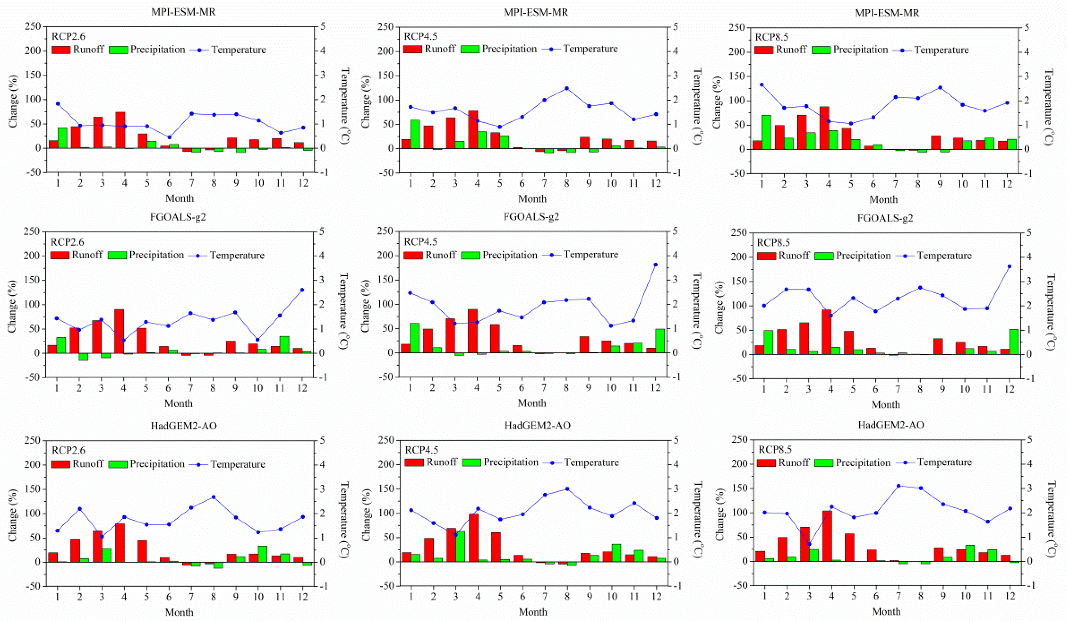
Figure 9 illustrates that the simulated runoff of the selected GCMs under the influence of climate change increases in the future period compared with the baseline period. Due to the uncertainty on the meteorological data for different GCMs, the runoff simulated with different input data from different GCMs shows obvious differences. Among the three GCMs, FGOALS-g2 provides the largest inter-annual change of runoff, followed by HadGEM2-AO with a very small difference, and the runoff of MPI-ESM-MR changed the least, with values of 30.89%, 30.34% and 26.73% respectively. The simulated monthly runoff shows the largest change in the “rcp8.5” emission scenario of MPI-ESM-MR and HadGEM2-AO, and in the “rcp4.5” emission scenario of FGOALS-g2, with the runoff rising by 29.98%, 34.28%, and 32.34%, respectively. The emission scenario that shows least change is “rcp4.5” in MPI-ESM-MR and HadGEM2-AO, and “rcp8.5” in FGOALS-g2, with the runoff rising by 25.82%, 30.62%, and 30.96 respectively, while the increase of 24.39%, 26.13%, and 29.36% in MPI-ESM-MR, HadGEM2-AO and FGOALS-g2, respectively, were seen in the runoff presented by the rest of the scenarios.
The runoff change is influenced by both the precipitation and temperature change. The precipitation increase results in the increase of the runoff, and the temperature increase causes the snowmelt increase, followed by the runoff increase. Meanwhile, the increase in temperature leads to the increasing evapotranspiration and then the declining runoff. Due to the combined influence of precipitation and temperature change, the sensitivity of runoff to the climatic variables is different in different months. The runoff change shows a relatively smaller rising range in autumn, and even a descending change in July and August in most scenarios. As precipitation exhibits a similar change, while the temperature increases more obviously compared with the runoff during the same period, the change of runoff in autumn is influenced by precipitation rather than temperature. It is indicated from Figure 9 that the runoff significantly increases from February to May, even reaching above 50% in some RCP scenarios, in the period of 2021–2060 compared with the baseline period. The change of precipitation and temperature does not significantly increase, and it even descends in some months. This is because, compared with precipitation and mean temperature, other meteorological variables such as effective accumulated temperature influence the runoff more significantly. The infiltration of surface water and runoff yield, which are related to the water-holding capacity of the soil on the underlying surface, are influenced by effective accumulated temperature above 0 °C with the soil freezing/thawing. The influence of effective accumulated temperature on runoff varies in different months, and it is greatest in the spring months, because the effective accumulated temperature influences the snowmelt most significantly in the spring season compared with other seasons [24]. In addition, the runoff is mainly supplied by groundwater recharge during the winter season when the precipitation and snowmelt are low. The groundwater recharge is not fully considered in the runoff simulation [47].
5. Conclusions
The historical annual and monthly series of precipitation and temperature data were used to study the climate change of the mountain area in the Manas River basin in the period from 1961 to 2015. A modified TOPMODEL with a snowmelt module was used for the runoff simulation with different future climate change scenarios for the period from 2021 to 2060. The study of the runoff change under the influence of climate change was carried out. The conclusions are summarized as follows:
- The annual runoff and climatic variables all show increasing trends during the period from 1961 to 2015. The abrupt change point of annual runoff (1995) is similar to the climatic variables (1992, 1994, 1993 and 1994 of annual precipitation, MAT, LAT, and HAT respectively). The runoff is supplied by precipitation rather than snowmelt in the winter season, and the opposite is true in the spring and autumn. During the summer season, the recharge of precipitation and snowmelt to runoff are almost identical.
- The bias-corrected monthly mean temperature data of the chosen GCMs, which are MPI-ESM-MR, FGOALS-g2, and HadGEM2-AO, from 2021 to 2160 all increase compared with the baseline period from 1961 to 2000. The monthly mean temperature increases the most in “rcp8.5”. “rcp4.5” showed the next largest increase, and “rcp2.6” increased the least in all chosen GCMs. The monthly precipitation presents the greatest increasing change in the winter season, and the descending change in December in the “rcp2.6” emission scenario of MPI-ESM-MR, the “rcp2.6” and “rcp8.5” emission scenarios of HadGEM2-AO, and in February in the “rcp2.6” emission scenario of FGOALS-g2.
- The monthly runoff from 2021 to 2060 simulated by the modified TOPMODEL with different emission scenarios in different GCMs all increase compared with the baseline period, and will increase by 24.39%, 25.82%, and 29.98% in “rcp2.6”, “rcp4.5”, and “rcp8.5” emission scenarios, respectively, of MPI-ESM-MR, 29.36%, 32.34%, and 30.96% of FGOALS-g2, and 26.13%, 30.62%, and 34.28% of HadGEM2-AO. The largest increasing change often occurs in April. The runoff increases significantly more from late winter to spring than in the other months.
In this paper, the study area is located in the upstream mountain area of the Manas River, where the effect of human activity is weak and climate change is the dominant influencing factor of the runoff. The human activity, such as underlying surface variation and artificial water distribution, was not considered in this research. The influence of climatic variables on runoff was analyzed independently. This research is limited to uncertainties caused during the numerical simulation study of the influence of climatic variables on runoff. Firstly, the correlation analysis between the runoff and climatic variables is based on the assumption that each climatic variable is independent of the others, as opposed to the reality. Secondly, the historical and future climatic data and mathematical statistics methods used in this study to analyze the hydrological and meteorological time series cause inevitable uncertainty, such as the bias correction method for the meteorological data in CMIP5. Moreover, the complexity and polytropy in nature make the climate change more complicated, and the climate change assessment more unreliable. Thirdly, a physics-based distributed hydrological model coupled with an energy balance snowmelt model should be developed to evaluate the influence of climatic variables on runoff more accurately in the future. Finally, further study should be carried out on the effect of climate change on unusual hydrological events instead of runoff, to reveal the response mechanism of hydrological factors to climate change. For this purpose, observations and experiments should be carried out to collect data to improve the accuracy of the hydrological model. The simulated runoff with the chosen GCMs reveals that, as the runoff significantly increases from February to May, there is an increase in the frequency of spring flood occurrence. It provides the management of the hydropower stations and reservoir group with important reference values. In summary, the conclusions provided in this research should be useful for the management of water resources in the Manas River basin.
Acknowledgments
This study was supported by the National Scientific Foundation of China (NSFC) (No. 41371052 and U1203282). Ministry of Water Resources’ special funds for scientific research on public causes (201501059).The authors are very grateful to the supporting sponsored by Qing Lan Project of Jiangsu Province and Jiangsu Province outstanding young teachers and principals overseas training program [2015]35.
Author Contributions
Lei Ren and Lian-qing Xue conceived and designed the research themes; Lei Ren, Jia Shi, Qiang Han and Peng-fei Yi analyzed the data; Jia Shi and Qiang Han contributed to data preparation; Lei Ren wrote the paper; Yuan-hong Liu made editing corrections and improvements to the manuscript. All authors have contributed to the revision and approved the manuscript. The authors thank Luo-chen Zhang, Yong-hong Chu, Chao Sun, et al., in Tarim River Basin Administration, who provided the hydrological data.
Conflicts of Interest
The authors declare no conflict of interest.
References
- Fu, G.B.; Charles, S.P.; Chiew, F.H.S. A two-parameter climate elasticity of streamflow index to assess climate change effects on annual streamflow. Water Resour. Res. 2007, 43, W11401. [Google Scholar] [CrossRef]
- Ralph, A.W.; Ranjan, S.M.; Felden, F. Incorporation of climate change in water availability modeling. J. Hydrol. Eng. 2005, 10, 375–385. [Google Scholar]
- Bronstert, A.; Kolokotronis, V.; Schwandt, D.; Straub, H. Comparison and evaluation of regional climate scenarios for hydrological impact analysis: General scheme and application example. Int. J. Climatol. 2007, 27, 1579–1594. [Google Scholar] [CrossRef]
- Chen, Y.; Takeuchi, K.; Xu, C.; Chen, Y.; Xu, Z. Regional climate change and its effects on river runoff in the Tarim Basin, China. Hydrol. Process. 2006, 20, 2207–2216. [Google Scholar] [CrossRef]
- Wu, C.H.; Huang, G.R.; Yu, H.J. Prediction of extreme floods based on CMIP5 climate models: A case study in the Beijiang River basin, South China. Hydrol. Earth Syst. Sci. 2015, 19, 1385–1399. [Google Scholar] [CrossRef]
- Ma, C.K.; Sun, L.; Liu, S.Y.; Shao, M.A.; Luo, Y. Impact of climate change on the streamflow in the glacierized Chu River Basin, Central Asia. J. Arid Land 2015, 7, 501–513. [Google Scholar] [CrossRef]
- Alfieri, L.; Burek, P.; Feyen, L.; Forzieri, G. Global warming increases the frequency of river floods in Europe. Hydrol. Earth Syst. Sci. 2015, 19, 2247–2260. [Google Scholar] [CrossRef]
- Jones, R.N.; Chiew, F.H.S.; Boughton, W.C.; Zhang, L. Estimating the sensitivity of mean annual runoff to climate change using selected hydrological models. Adv. Water Resour. 2006, 29, 1419–1429. [Google Scholar] [CrossRef]
- Legesse, D.; Abiye, T.A.; Vallet-Coulomb, C.; Abate, H. Streamflow sensitivity to climate and land cover changes: Meki River, Ethiopia. Hydrol. Earth Syst. Sci. 2010, 14, 2277–2287. [Google Scholar] [CrossRef]
- Dan, L.; Ji, J.J.; Xie, Z.H.; Chen, F.; Wen, G.; Richey, J.E. Hydrological projections of climate change scenarios over the 3H region of China: A VIC model assessment. J. Geophys. Res. Atmos. 2012, 117. [Google Scholar] [CrossRef]
- Kabiri, R.; Bai, V.R.; Chan, A. Assessment of hydrologic impacts of climate change on the runoff trend in Klang Watershed, Malaysia. Environ. Earth Sci. 2015, 73, 27–37. [Google Scholar] [CrossRef]
- Lopez, S.R.; Hogue, T.S.; Stein, E.D. A framework for evaluating regional hydrologic sensitivity to climate change using archetypal watershed modeling. Hydrol. Earth Syst. Sci. 2013, 17, 3077–3094. [Google Scholar] [CrossRef]
- Wang, W.G.; Wei, J.D.; Shao, Q.X.; Xing, W.Q.; Yong, B.; Yu, Z.B.; Jiao, X.Y. Spatial and temporal variations in hydro-climatic variables and runoff in response to climate change in the Luanhe River basin, China. Stoch. Environ. Res. Risk Assess. 2015, 29, 1117–1133. [Google Scholar] [CrossRef]
- Sun, W.C.; Wang, J.; Li, Z.J.; Yao, X.L.; Yu, J.S. Influences of climate change on water resources availability in Jinjiang Basin, China. Sci. World J. 2014, 2014, 908349. [Google Scholar] [CrossRef] [PubMed]
- Zhao, J.; Shi, Y.F.; Huang, Y.S.; Fu, J.W. Uncertainties of snow cover extraction caused by the nature of topography and underlying surface. J. Arid Land 2015, 7, 285–295. [Google Scholar] [CrossRef]
- Luo, Y.; Arnold, J.; Liu, S.Y.; Wang, X.Y.; Chen, X. Inclusion of glacier processes for distributed hydrological modeling at basin scale with application to a watershed in Tianshan Mountains, northwest China. J. Hydrol. 2013, 477, 72–85. [Google Scholar] [CrossRef]
- Ling, H.B.; Xu, H.L.; Fu, J.Y.; Liu, X.H. Surface runoff processes and sustainable utilization of water resources in Manas River Basin, Xinjiang, China. J. Arid Land 2012, 4, 271–280. [Google Scholar] [CrossRef]
- Shi, Y.; Shen, Y.; Kang, E.; Li, D.; Ding, Y.; Zhang, G.; Hu, R. Recent and future climate change in northwest china. Clim. Chang. 2007, 80, 379–393. [Google Scholar] [CrossRef]
- He, X.L.; Guo, S.L. Impacts of climate change on hydrology and water resources in the Manas River Basin. Adv. Water Sci. 1998, 9, 77–83. [Google Scholar]
- Wu, J.; Gao, X.J. A Gridded daily observation dataset over china region and comparison with the other datasets. Chin. J. Geophys. 2013, 56, 1102–1111. (In Chinese) [Google Scholar]
- Taylor, K.E.; Stouffer, R.J.; Meehl, G.A. An Overview of CMIP5 and the Experiment Design. Bull. Am. Meteorol. Soc. 2012, 93, 485–498. [Google Scholar] [CrossRef]
- Li, L.; Simonovic, S.P. System dynamics model for predicting floods from snowmelt in North American prairie watersheds. Hydrol. Process. 2002, 16, 2645–2666. [Google Scholar] [CrossRef]
- Zhang, Y.C.; Li, B.L.; Bao, A.M.; Zhou, C.H.; Chen, X.; Zhang, X.R. Study on snowmelt runoff simulation in the Kaidu River basin. Sci. China Ser. D 2007, 50, 26–35. [Google Scholar] [CrossRef]
- Li, X.M.; Zhang, F.Y.; Shang, M.; Abduweli, J.; Li, L.H. Path analysis on impacts of meterological factors on runoff from tianshan mountains: A case study on Manas River and Kaidu River watersheds. Resour. Sci. 2012, 34, 652–659. (In Chinese) [Google Scholar]
- Xu, C.H.; Wang, F.T.; Li, Z.Q.; Wang, L.; Wang, P.Y. Glacier variation in the Manas River Basin during the period from 1972 to 2013. Arid Zone Res. 2016, 33, 628–635. (In Chinese) [Google Scholar]
- ESGF Node at DKRZ. Available online: https://esgf-data.dkrz.de/projects/esgf-dkrz/ (accessed on 31 March 2017).
- Zhang, Y.W.; Zhang, L.; Xu, Y. Simulations and projections of the surface air temperature in China by CMIP5 models. Clim. Chang. Res. 2016, 12, 10–19. (In Chinese) [Google Scholar]
- Chen, X.C.; Xu, Y.; Xu, C.H.; Yao, Y. Assessment of Precipitation Simulations in China by CMIP5 Multi-models. Prog. Inquis. Mutat. Clim. 2014, 10, 217–225. (In Chinese) [Google Scholar]
- Zhang, B.; Gong, Y.F.; Xu, Y.; Zhang, S. Evaluation on the simulation of the drought change in China based on global climate models from CMIP5. J. Arid Meteorol. 2014, 32, 694–700. (In Chinese) [Google Scholar]
- Serrano, V.L.; Mateos, V.L.; Garcia, J.A. Trend analysis of monthly precipitation over the Iberian Peninsula for the period 1865–2002. Hydrol. Process. 1999, 23, 1147–1157. [Google Scholar]
- Kendall, M.G. Rank Correlation Methods; Charles Griffin: London, UK, 1975. [Google Scholar]
- Mann, H.B. Nonparametric tests against trend. Econometrica 1945, 13, 245–259. [Google Scholar] [CrossRef]
- Serrano, A.; Mateos, V.L.; Garcia, J.A. Trend analysis of monthly precipitation over the Iberian Peninsula for the period 1921–1995. Phys. Chem. Earth Part B 1999, 24, 85–90. [Google Scholar] [CrossRef]
- Iman, R.L.; Helton, J.C. An investingation of uncertainty and sensitivity analysis techniques for computer models. Risk Anal. 1988, 8, 71–90. [Google Scholar] [CrossRef]
- Su, B.D.; Huang, J.L.; Gemmer, M.; Jian, D.N.; Tao, H.; Jiang, T.; Zhao, C.Y. Statistical downscaling of CMIP5 multi-model ensemble for projected changes of climate in the Indus River Basin. Atmos. Res. 2016, 178, 138–149. [Google Scholar] [CrossRef]
- Li, H.B.; Sheffield, J.; Wood, E.F. Bias correction of monthly precipitation and temperature fields from Intergovernmental Panel on Climate Change AR4 models using equidistant quantile matching. J. Geophys. Res. Atmos. 2010, 115. [Google Scholar] [CrossRef]
- Braithwaite, R.J. Calculation of degree-days for glacier-climatic research. Z. Gletsch. Glaziageol. 1984, 20, 1–8. [Google Scholar]
- Braithwaite, R.J.; Olesen, O.B. Calculation of glacier ablation from air temperature. In Glacier Fluctuation and Climate Change; Kluwer Academic Publishers: Dordrecht, The Netherlands, 1989; pp. 219–233. [Google Scholar]
- Cui, Y.H.; Ye, B.S.; Wang, J.; Liu, Y.C.; Jing, Z.F. Analysis of the spatial-temporal variations of the positive degree-day factors on the Glacier No. 1 at the headwaters of the Ürümqi River. J. Glaciol. Geocryol. 2010, 32, 265–274. (In Chinese) [Google Scholar]
- Quinn, P.; Beven, K.J.; Lamb, R. The ln(α/tanβ) index: How to calculate it and how to use it in the TOPMODEL framework. Hydrol. Process. 1995, 9, 161–182. [Google Scholar] [CrossRef]
- Beven, K.J.; Lamb, R.; Quinn, P.F.; Romanowicz, R.; Freer, J. TOPMODEL. In Computer Models of Watershed Hydrology; Singh, V.P., Ed.; Water Resources Publications: Douglas County, CO, USA, 1995; pp. 627–668. [Google Scholar]
- Beven, K.J.; Kirkby, M.J. A physically based variable contributing area model of basin hydrology. Hydrol. Sci. Bull. 1979, 24, 43–69. [Google Scholar] [CrossRef]
- Manandhar, S.; Pandey, V.P.; Ishidaira, H.; Kazama, F. Perturbation study of climate change impacts in a snow-fed river basin. Hydrol. Process. 2013, 27, 3461–3474. [Google Scholar] [CrossRef]
- Neary, V.S.; Habib, E.; Fleming, M. Hydrologic modeling with NEXRAD precipitation in middle Tennessee. J. Hydrol. Eng. 2004, 9, 339–349. [Google Scholar] [CrossRef]
- Nash, J.E.; Sutcliffe, J.V. River flow forecasting through conceptual models. Part I: A discussion of principles. J. Hydrol. 1970, 10, 282–290. [Google Scholar] [CrossRef]
- Geospacial Data Cloud. Available online: http://www.gscloud.cn/ (accessed on 31 March 2017).
- Zeng, X.; Lyu, J.H.; Shi, W.J. Analysis on runoff and flood characteristics of Manas River. J. Shihezi Univ. (Nat. Sci.) 2006, 24, 346–349. (In Chinese) [Google Scholar]
Figure 1.
Location of the Manas River basin.
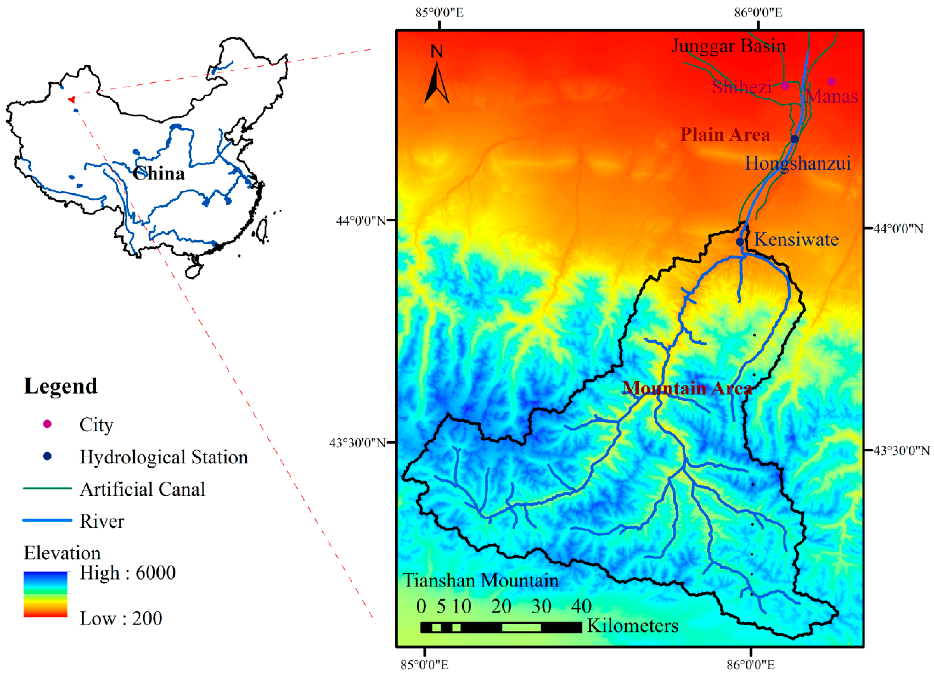
Figure 2.
Nonparametric Mann-Kendall (MK) test and liner regression analysis of annual runoff.
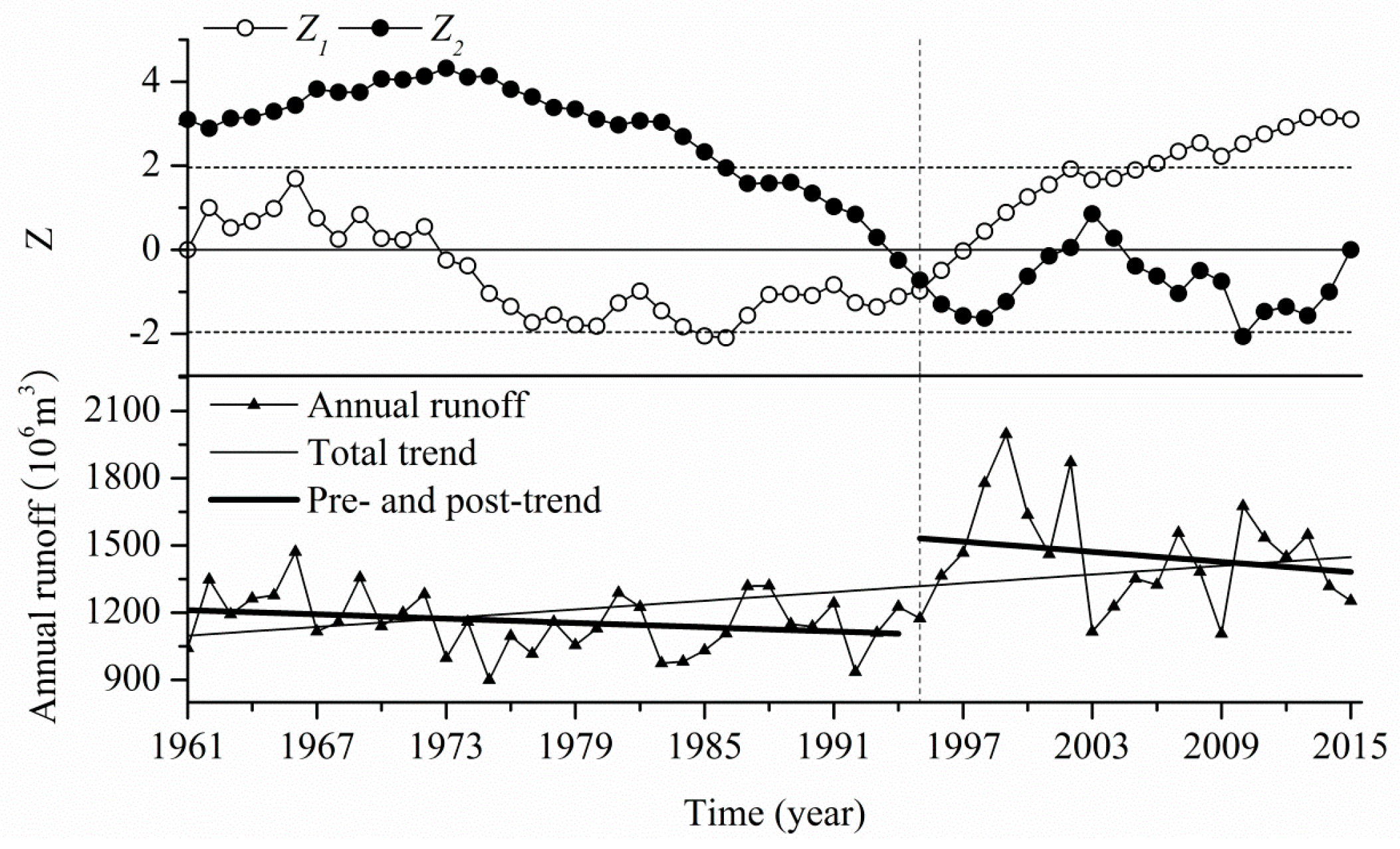
Figure 3.
Nonparametric MK test and liner regression analysis of (a) annual precipitation and (b) temperature (mean annual temperature (MAT), lowest annual temperature (LAT), and highest annual temperature (HAT)).
Figure 3.
Nonparametric MK test and liner regression analysis of (a) annual precipitation and (b) temperature (mean annual temperature (MAT), lowest annual temperature (LAT), and highest annual temperature (HAT)).
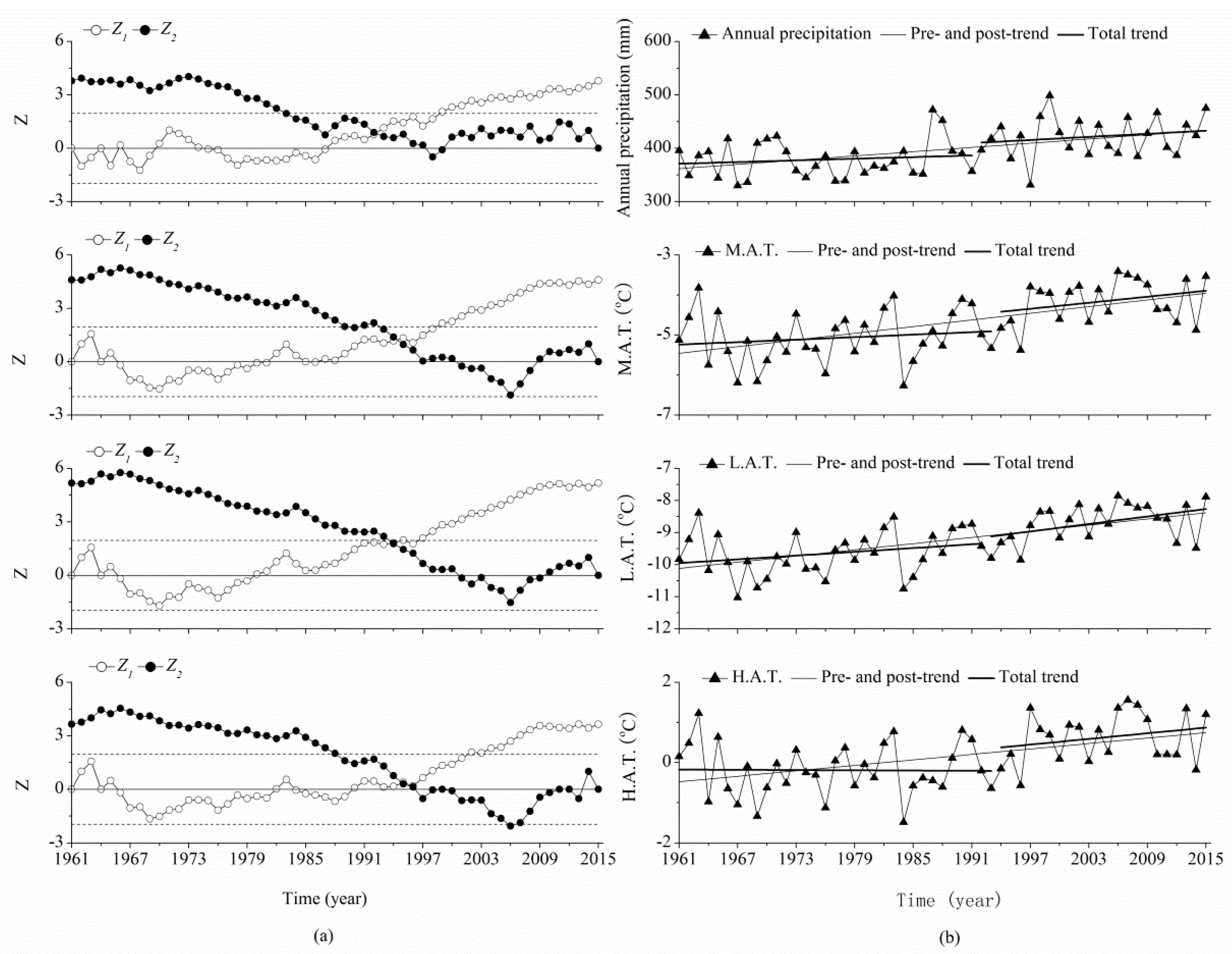
Figure 4.
Relationship curve of the topographical index and area ratio.
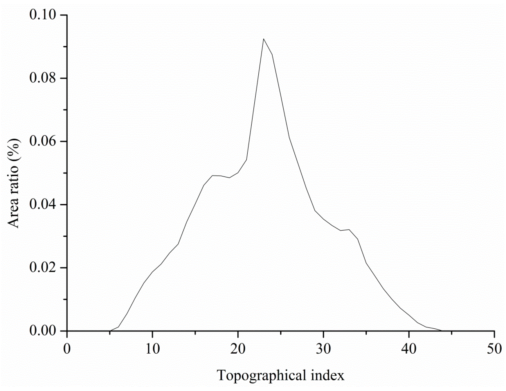
Figure 5.
Mean monthly runoff in log-scale and precipitation during the calibration (2001–2010) and validation (2011–2015) period.
Figure 5.
Mean monthly runoff in log-scale and precipitation during the calibration (2001–2010) and validation (2011–2015) period.
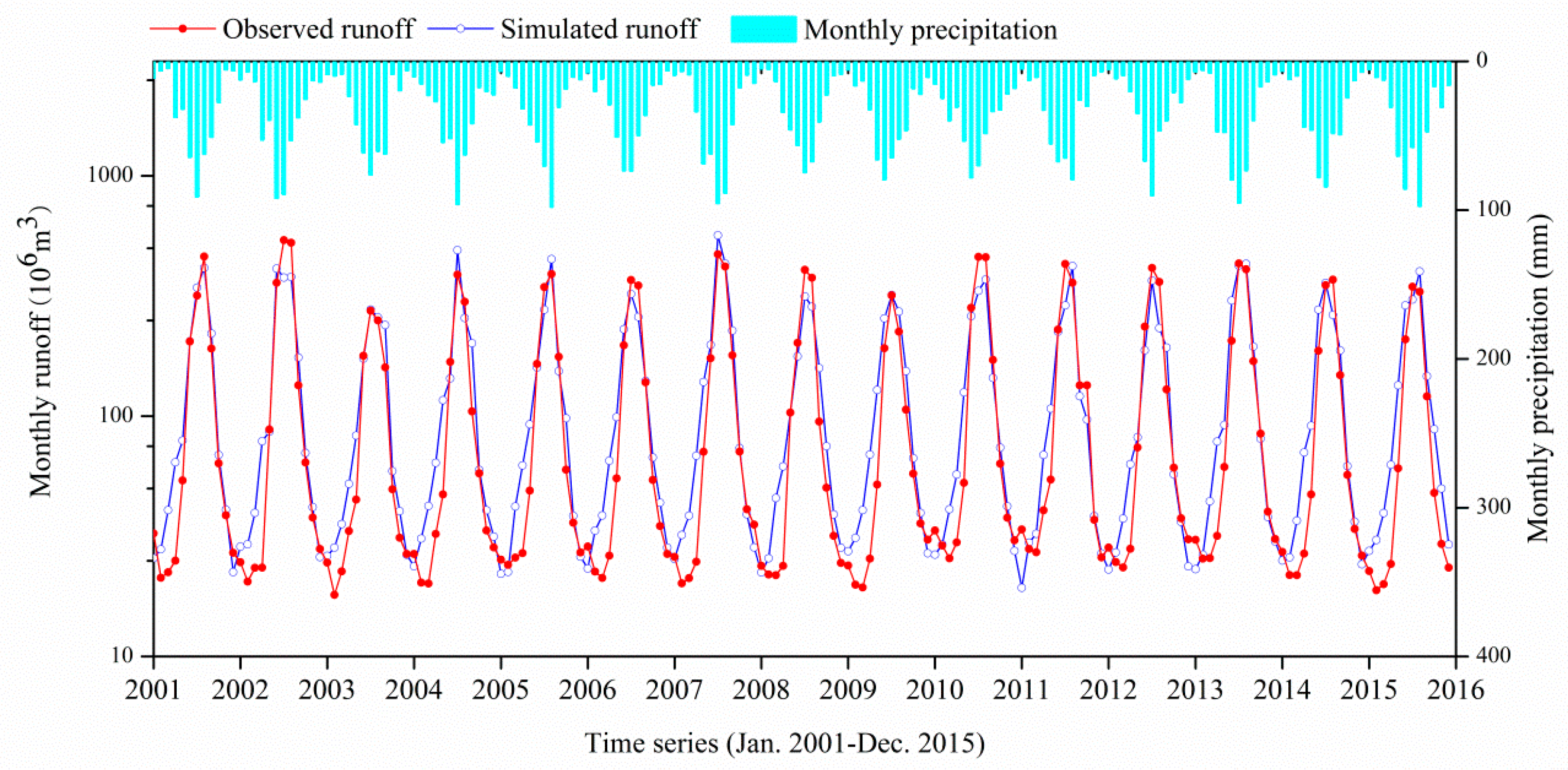
Figure 6.
Average monthly precipitation and temperature data of global climate models (GCMs) before and after bias correction.
Figure 6.
Average monthly precipitation and temperature data of global climate models (GCMs) before and after bias correction.
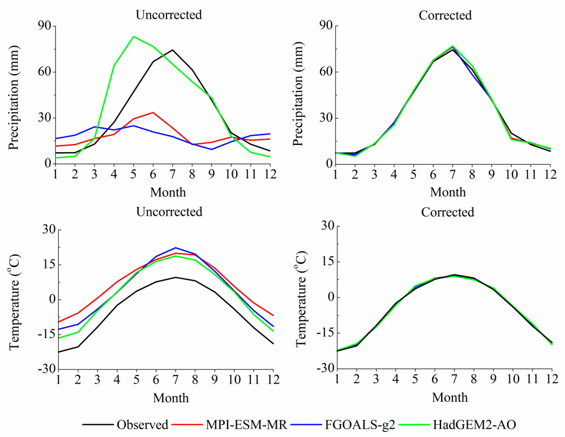
Figure 7.
The bias corrected projected annual precipitation and temperature time series during the period from 1961 to 2100.
Figure 7.
The bias corrected projected annual precipitation and temperature time series during the period from 1961 to 2100.
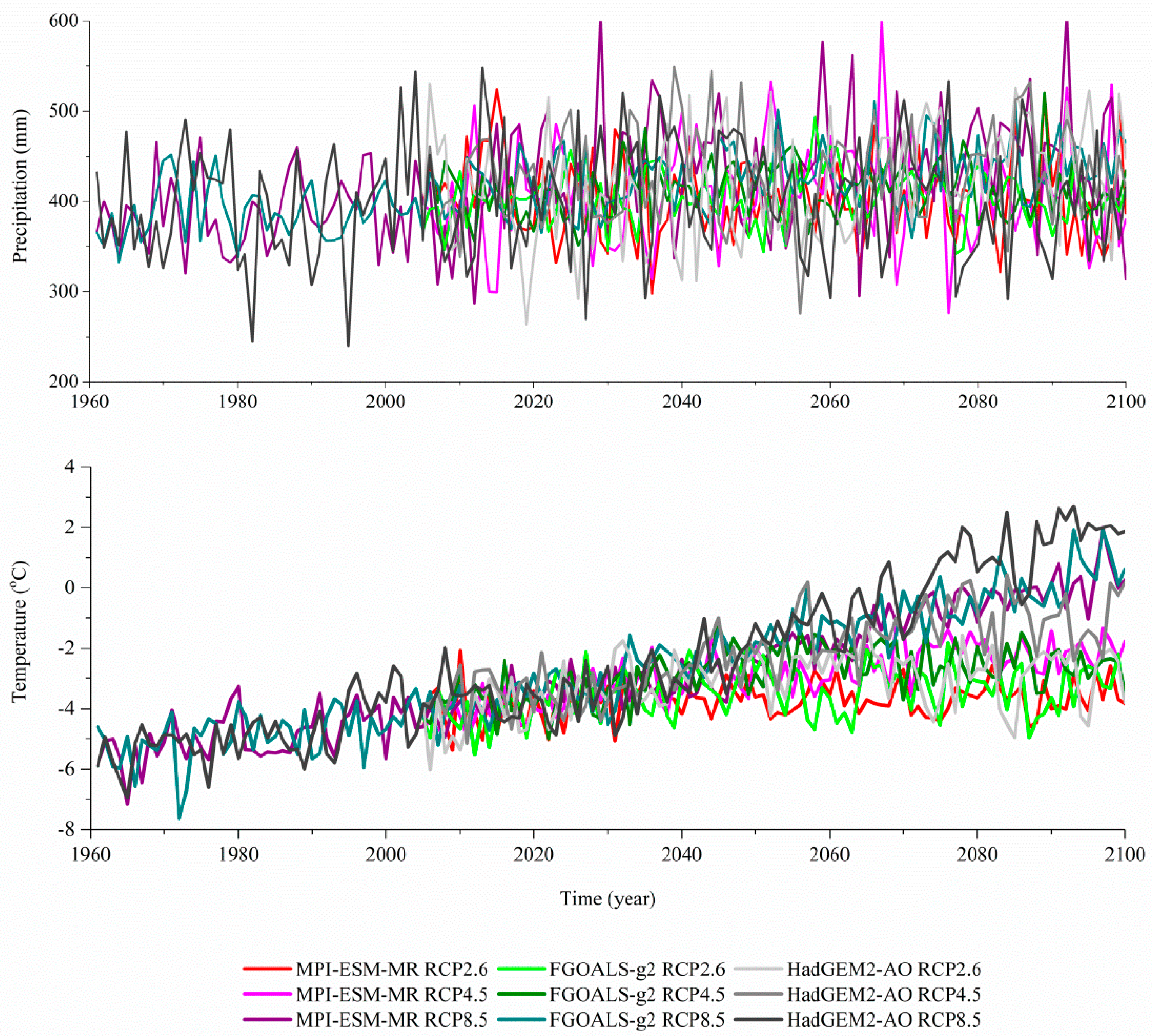
Figure 8.
Monthly mean precipitation and temperature changes in the future during the period from 2021 to 2060.
Figure 8.
Monthly mean precipitation and temperature changes in the future during the period from 2021 to 2060.
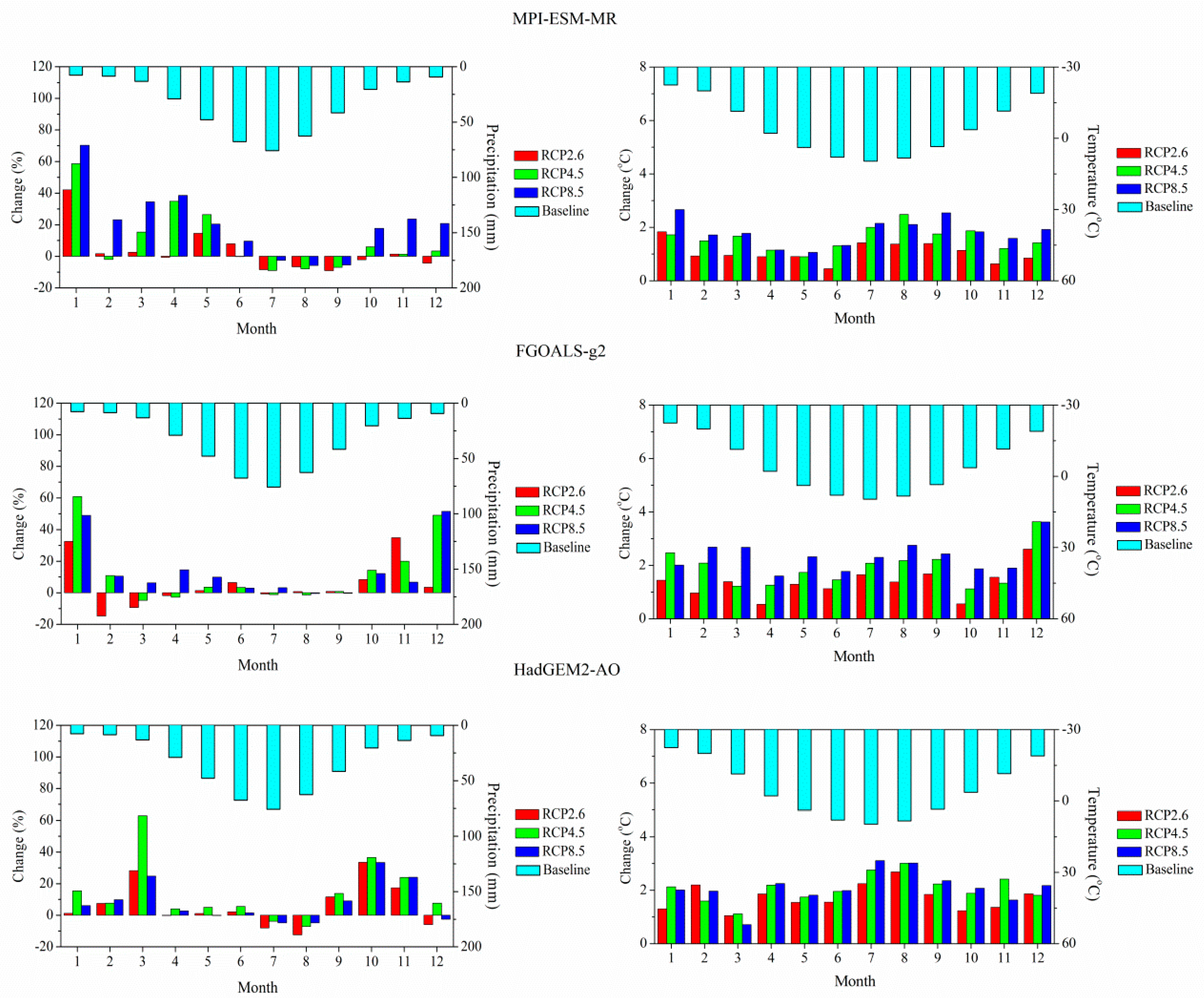
Figure 9.
Comparison of average monthly runoff, precipitation, and temperature change.


Table 1.
Results of MK tests for annual runoff, annual precipitation and temperature (MAT, LAT and HAT).
Table 1.
Results of MK tests for annual runoff, annual precipitation and temperature (MAT, LAT and HAT).
| Analysis Item | Data Period | Z | Critical Value | Significant Trend |
|---|---|---|---|---|
| Annual runoff | 1961–2015 | 3.09 | (−1.96, 1.96) | Increasing |
| Annual precipitation | 1961–2015 | 3.78 | (−1.96, 1.96) | Increasing |
| MAT | 1961–2015 | 4.59 | (−1.96, 1.96) | Increasing |
| LAT | 1961–2015 | 5.17 | (−1.96, 1.96) | Increasing |
| HAT | 1961–2015 | 3.64 | (−1.96, 1.96) | Increasing |
Table 2.
Results of abrupt change of annual runoff, annual precipitation and temperature (MAT, LAT and HAT).
Table 2.
Results of abrupt change of annual runoff, annual precipitation and temperature (MAT, LAT and HAT).
| Analysis Item | Change Point | Pre-Trend Rate * | Post-Trend Rate ** | Total Trend Rate *** | Change **** |
|---|---|---|---|---|---|
| Annual runoff | 1995 | −3.1852 | −7.5200 | 6.4981 | −4.3348 |
| Annual precipitation | 1992 | 0.5155 | 0.9611 | 1.3244 | 0.4456 |
| MAT | 1994 | 0.0103 | 0.0250 | 0.0278 | 0.0147 |
| LAT | 1993 | 0.0196 | 0.0389 | 0.0321 | 0.0193 |
| HAT | 1994 | −0.0010 | 0.0236 | 0.0227 | 0.0246 |
Notes: *, **, *** the pre-, post-, and total trend rate for annual runoff, annual precipitation, MAT, LAT, and HAT are in 10 × 106 m3/year, mm/year, °C/year, °C/year, and °C/year, respectively; the negative value stands for a decreasing trend and the positive value stands for a rising trend; **** change between pre- and post-trend rates with positive values are increases in change and negative values are decreases in change; the metering unit is the same as the trend rate.
Table 3.
Partial Correlation Coefficients (PCC) between runoff and climatic variables during the period of 1961–2015.
Table 3.
Partial Correlation Coefficients (PCC) between runoff and climatic variables during the period of 1961–2015.
| Time | Precipitation | Mean Temperature | Lowest Temperature | Highest Temperature |
|---|---|---|---|---|
| January | 0.3736 * | 0.0054 | 0.0325 | −0.0568 |
| February | 0.3156 * | 0.1718 | 0.2157 | 0.1032 |
| March | 0.0451 | 0.2050 | 0.1456 | 0.2540 |
| April | 0.1179 | 0.3773 * | 0.3960 * | 0.3793 * |
| May | −0.0175 | 0.4937 * | 0.5156 * | 0.4665 * |
| June | 0.3158 * | 0.3474 * | 0.4705 * | 0.2699 * |
| July | 0.4263 * | 0.3619 * | 0.6187 * | 0.2308 |
| August | 0.4679 * | 0.4378 * | 0.5682 * | 0.3204 * |
| September | 0.2067 | 0.5131 * | 0.5717 * | 0.4330 * |
| October | 0.2138 | 0.3240 * | 0.3437 * | 0.2963 * |
| November | 0.0213 | 0.2757 * | 0.2652 | 0.2340 |
| December | 0.4008 * | 0.2447 | 0.2358 | 0.1955 * |
| Spring | 0.0817 | 0.3147 * | 0.3064 * | 0.3169 * |
| Summer | 0.6116 * | 0.4690 * | 0.6085 * | 0.3564 * |
| Autumn | 0.1186 | 0.5379 * | 0.5387 * | 0.4850 * |
| Winter | 0.5797 * | 0.1644 | 0.2149 | 0.0595 |
| Annual | 0.5704 | 0.4368 * | 0.4716 * | 0.3681 * |
Note: * means the correlation is significant at 95% confidence level.
© 2017 by the authors. Licensee MDPI, Basel, Switzerland. This article is an open access article distributed under the terms and conditions of the Creative Commons Attribution (CC BY) license (http://creativecommons.org/licenses/by/4.0/).
Share and Cite
MDPI and ACS Style
Ren, L.; Xue, L.-q.; Liu, Y.-h.; Shi, J.; Han, Q.; Yi, P.-f. Study on Variations in Climatic Variables and Their Influence on Runoff in the Manas River Basin, China. Water 2017, 9, 258. https://doi.org/10.3390/w9040258
AMA Style
Ren L, Xue L-q, Liu Y-h, Shi J, Han Q, Yi P-f. Study on Variations in Climatic Variables and Their Influence on Runoff in the Manas River Basin, China. Water. 2017; 9(4):258. https://doi.org/10.3390/w9040258
Chicago/Turabian StyleRen, Lei, Lian-qing Xue, Yuan-hong Liu, Jia Shi, Qiang Han, and Peng-fei Yi. 2017. "Study on Variations in Climatic Variables and Their Influence on Runoff in the Manas River Basin, China" Water 9, no. 4: 258. https://doi.org/10.3390/w9040258
Note that from the first issue of 2016, this journal uses article numbers instead of page numbers. See further details here.