Article

Comparative Study on the Selection Criteria for Fitting Flood Frequency Distribution Models with Emphasis on Upper-Tail Behavior

1
Center for Water Resources and Environment, Sun Yat-sen University, Guangzhou 510275, China
2
Key Laboratory of Water Cycle and Water Security, Southern China of Guangdong High Education Institute, Sun Yat-sen University, Guangzhou 510275, China
3
CSIRO Mathematics, Informatics and Statistics, Private Bag No 5, Wembley 6913, Australia
4
State Key Laboratory of Hydrology–Water Resources and Hydraulic Engineering, Hohai University, Nanjing 210098, China
5
Department of Geosciences, University of Oslo, Oslo N-0316, Norway
6
Institute of Tropical Agriculture and Forestry, Hainan University, Haikou 570228, China
*
Author to whom correspondence should be addressed.
Water 2017, 9(5), 320; https://doi.org/10.3390/w9050320
Submission received: 21 February 2017 / Revised: 24 April 2017 / Accepted: 25 April 2017 / Published: 2 May 2017

Abstract

:
The upper tail of a flood frequency distribution is always specifically concerned with flood control. However, different model selection criteria often give different optimal distributions when the focus is on the upper tail of distribution. With emphasis on the upper-tail behavior, five distribution selection criteria including two hypothesis tests and three information-based criteria are evaluated in selecting the best fitted distribution from eight widely used distributions by using datasets from Thames River, Wabash River, Beijiang River and Huai River. The performance of the five selection criteria is verified by using a composite criterion with focus on upper tail events. This paper demonstrated an approach for optimally selecting suitable flood frequency distributions. Results illustrate that (1) there are different selections of frequency distributions in the four rivers by using hypothesis tests and information-based criteria approaches. Hypothesis tests are more likely to choose complex, parametric models, and information-based criteria prefer to choose simple, effective models. Different selection criteria have no particular tendency toward the tail of the distribution; (2) The information-based criteria perform better than hypothesis tests in most cases when the focus is on the goodness of predictions of the extreme upper tail events. The distributions selected by information-based criteria are more likely to be close to true values than the distributions selected by hypothesis test methods in the upper tail of the frequency curve; (3) The proposed composite criterion not only can select the optimal distribution, but also can evaluate the error of estimated value, which often plays an important role in the risk assessment and engineering design. In order to decide on a particular distribution to fit the high flow, it would be better to use the composite criterion.

1. Introduction

Flood frequency analysis plays a key role and is a constant topic in hydrology and water resources, especially for hydraulic design and flood hazard mitigation and management (e.g., [1,2]). Adequate estimations of extreme annual maximum daily flow are very important for flood control in which the upper-tail behavior of the flood frequency distribution is the key [3,4]. The frequency analysis of hydrological extremes requires a fit of a probability distribution to the observed data in order to suitably represent the frequency of occurrence of rare events [5]. More than 20 statistical distributions have been used as the flood frequency distributions [3]. Statistical criteria must be used to determine the suitable distribution for flood frequency analysis [6]. However, for a given region, different model selection methods often result in different optimal distributions, especially when the focus is on the upper tail of flood frequency distribution [7]. The flood estimation vary widely for different distributions. Therefore, the most suitable distribution must be chosen.
There are mainly two kinds of model selection techniques: hypothesis tests based on goodness-of-fit and information-based criteria [5]. The commonly used hypothesis tests are the Kolmogorov–Smirnov (KS) test, Anderson–Darling (AD) test, probability plot correlation coefficient (PPCC), chi-squared test and log-likelihood ratio tests (t-test and F-test). Information-based criteria include the Akaike Information Criterion [8], Akaike Information Criterion–second order variant (AICc) and Bayesian Information Criterion (BIC).
There have been some studies in the past on the comparison of various model selection methods. The choice of a distribution for flood frequency should be based on features reflecting the upper tail shape [9]. However, there are rare studies about the comparison of model selection criteria with emphasis on the upper tail of flood frequency distribution. Cicioni et al. (1973) considered the two-parameter lognormal (LN2), three-parameter log-normal (LN3), Pearson type III distribution (P3) and Generalized Extreme Value (GEV) distributions for the flood data from 108 stations in Italy with record length of more than 27 years, and used Chi-squared, KS, Cramer–Von Mises and AD tests for distribution selection, giving the result that the Chi-squared test selected LN2 but other tests selected GEV [7]. Haktanir and Horlacher (1993) applied a statistical model comprising nine different probability distributions for flood frequency analysis of annual flood peak series for 11 unregulated streams [10]. The distributions were compared by classical goodness-of-fit tests (GOFT) on the observed series. However, different classical goodness-of-fit tests often result in different distributions for a specific region. Haddad et al. (2012) presented a case study with flood data from Tasmania in Australia in order to select the best fit flood frequency distribution by examining four model selection criteria: AIC, AICc, BIC and a modified Anderson–Darling (AD) Criterion [11]. It was found from the Monte Carlo simulation that AD is more successful in correctly recognizing the parent distribution than AIC and BIC when the parent is a three-parameter distribution. On the other hand, AIC and BIC are better at correctly recognizing the parent distribution when the parent is a two-parameter distribution. Baldassarre (2009) demonstrated that model selection criteria such as AIC, BIC and AD which are seldom used in hydrological applications, can help to identify the best probability model [12]. These three methods were compared through an extensive numerical analysis by using synthetic data samples. The model selection criteria based on AIC, BIC and AD were also adopted by Laio et al. (2009) and Calenda et al. (2009) [5,13], with further investigation to verify which of the selection criteria is more efficient, especially in the case of small samples and heavy tailed distributions, as these are commonly encountered in flood frequency analysis. The studies were carried out by a Monte Carlo simulation to investigate the robustness of the model selection criteria in recognizing the real parent distributions. Overall, none of the classical hypothesis tests and information-based criteria can be used as a universal indicator to select the suitable distributions for different stations around the world. Burnham and Anderson (2002) indicated that the hypothesis test and information-based approaches have different selection frequencies [14]. Even if the same parameter estimation method is used, different model selection criteria result in different optimal distributions. This is perhaps because each type of model selection criteria has its own characteristics and applicable scope [15]. Therefore, it is not surprising that the results of these tests are not always in agreement.
Estimating the magnitude and frequency of large floods is difficult and involves a large degree of uncertainty, especially when the flow record is of limited length. The Monte Carlo method and Paleohydrologic techniques offer a way to lengthen a short-term data record and, to reduce the uncertainty in hydrologic analysis [16,17,18].
The basic assumption of traditional frequency analysis methods is that the hydrological data used are stationary, independent and identically distributed over time. However, in the past decades this stationarity assumption has been severely challenged because global climate change [19] and/or large-scale human activities [20] have altered the statistical characteristics of hydrological processes [21]. Some hydrologists have declared that “stationarity is dead” [22], and suggest that nonstationary probabilistic models need to be identified and possibly used in some practical cases when the characteristics of hydrological processes have been significantly changed [23,24,25].
Selection of a flood frequency distribution is a necessary step in flood frequency analysis. However, selection of the best fit distribution from a large number of candidate distributions available in the literature is a difficult task. There are two reasons behind having no unique probability distributions for a given region. (1) Flood characteristics are different in different rivers; (2) there is a lack of an effective model selection criterion to be used to determine the suitable distribution for flood frequency analysis.
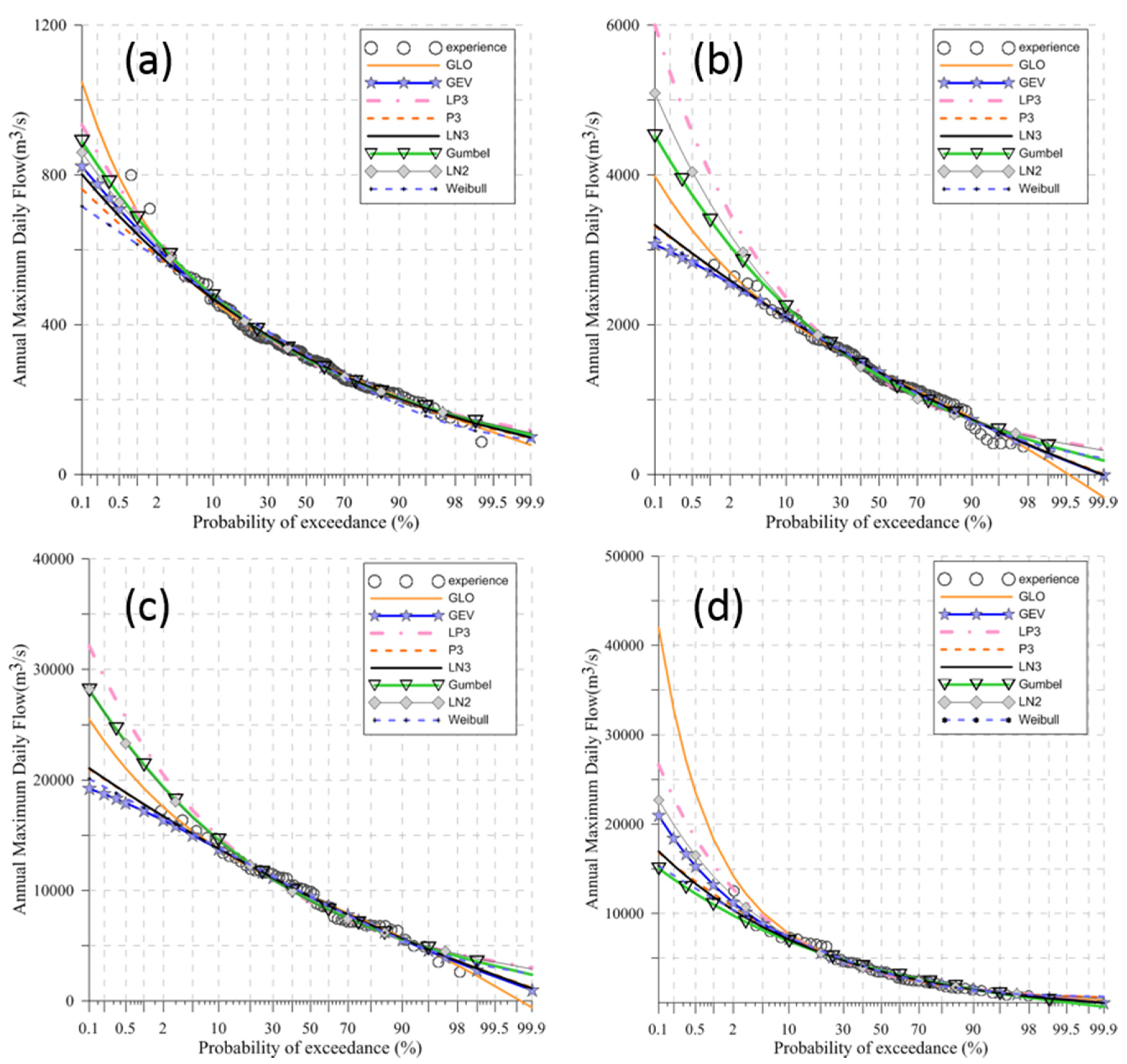
Flood frequency curves of different distributions show differences mainly at the tails of the distributions, especially at the high flow part which generally shows big differences for different distributions [10]. Hosking and Wallis (1986) argued that the choice of a distribution for flood frequency should be based on features reflecting the upper tail shape [9]. The observed flow data at the high flow part play an important role in the flood frequency analysis and should be addressed in the goodness-of-fit. The question is which model selection criterion can be a good indicator of the goodness of prediction for the extreme upper tail quantiles such as return periods of 100 years or more. In order to determine the more efficient model selection criterion which focuses on the upper-tail behaviour and reduces the influence of the lower tail end, a new composite criterion method to identify the optimal distribution is proposed in this study. The composite criterion can evaluate the goodness of predictions of the extreme upper-tail events carried out using synthetic samples of data by Monte Carlo simulation with Kappa distribution as the parent distribution. Stochastic simulation is widely applied for estimating the design flood of various hydrological systems.
In order to reveal the best fitted distribution for different regions in the flood frequency analysis with emphasis on the upper-tail behavior, the study aims at clarifying how the model selection methods work in different situations in the flood frequency analysis by (1) verifying whether hypothesis tests or information-based criteria methods are more efficient at the high flow part by clarifying the characteristic of model selection methods, and (2) trying to establish a composite of model selection criteria methods which can meet the demand of the engineering design. The findings from this study will benefit hazard mitigation and water resources management.

2. Methodology

2.1. Typical Probability Distributions

Many probability distributions (PDs) have been considered, in different situations, for the probabilistic model of extreme events, including P3, LP3, LN2, LN3, Gumbel (Extreme value type I, EV1), Weibull (Extreme value type III), GEV and Generalized logistic distribution (GLO). Rao and Hamed (2000) and Reiss and Thomas (2001) provided details of their probability density functions [26,27]. Eight well-known flood frequency probability distributions were used in this study. Two of them have two parameters (LN2 and Gumbel) and six have three parameters (LN3, Weibull, GEV, GLO, P3 and LP3). Two of them are heavy tail distributions (GLO and LP3), i.e., distribution tends to have large values with outliers (very high values); an often used definition of heavy tailed distributions is based on the fourth central moment [28]; four of them are mixed tail distributions (GEV, Gumbel, LN3 and LN2) and the other two are light tail distributions (P3, Weibull which can also be subexponential). More details regarding the tail of the PDs can be found in, for example, Adlouni et al. (2008) [28].

2.2. Model Selection Methods

There are mainly two kinds of model selection techniques: hypothesis tests based on goodness-of-fit and information-based criteria [5]. The traditional hypothesis testing methods are KS and AD [7]. KS and AD methods involve the confidence level and threshold (p values). If the p value is greater than the confidence level (typically 0.05), the original hypothesis is accepted as the data obeys the distribution, otherwise the original hypothesis is rejected. It was found from related researches that information-based criteria (AIC, BIC and AICc) can help to identify the best probability model in certain situations [11,12]. With respect to the distribution selection, two hypothesis tests (KS and AD) and three information-based criteria (AIC, BIC and AICc) are used in this paper (Table 1). The distributions are ranked according to their performances against each test or criterion. The best fitted distributions are the ones which perform in the top three of all the tests and criteria. Specific steps of computing the information-based criteria for each probability model are as follows.
(1)
The log-likelihood function value for each probability model was computed according to Table 1. Where parameters P (scale, location, shape) are the parameter values that maximize the log-likelihood function. The estimation method for parameter P of flood frequency probability models is the maximum likelihood, which was used to compute the log-likelihood function for each probability model.
(2)
The values of AIC, BIC, AICc can be computed according to Table 1 on the basis of the value of log-likelihood function and the number of parameters.

2.3. Parameter Estimation

The most common parameter estimation methods in flood frequency analysis are moments and the maximum likelihood [29]. Because the maximum likelihood estimation (MLE) generally shows less bias than other methods and provides a more consistent result to parameter estimation, it is recommended by Federal Emergency Management Agency of the United States (FEMA)’s guideline (2004) [30]. Therefore, in this paper, the MLE method was used for parameter estimation. More details regarding methods on parameter estimation can be found in, for example, Martins and Stedinger (2000), Hirose (1996), and Otten and Montfort (1980) [31,32,33].

2.4. Rigorous Program to Select the Optimal Distribution by Hypothesis Tests and Information-Based Criteria

In order to perform more rigorous and systematical analysis, we only present the first two optimal distributions for the hypothesis test and the information-based criteria. This is achieved through a rigorous program in finding the two optimal distributions from the candidate distributions. The procedure is demonstrated here by taking the information-based criteria as an example.
(1)
The candidate distributions are ordered from most to least favourite with AIC, BIC, AICc criteria. If the first distribution with the highest number of occurrences was selected respectively by AIC, BIC, AICc, then it is selected as the first optimal distribution of the information criteria.
(2)
After selecting the first optimal distribution, it is removed from the candidate distributions. Repeat step (1) to find the best distribution from the remaining distributions as the second optimal distribution.
(3)
In step (1), if two or more distributions have the same number of times appearing at the first position, then they will be sorted by the total number of occurrences in the preferred distribution (two or more distributions) selected respectively by AIC, BIC, AICc; the distribution with more occurrences is preferred.

2.5. Composite Criterion for Model Selection with Focus on the High Flow Part

An additional composite model selection criterion, based on an extensive numerical analysis by using synthetic data samples, is proposed here. Because the choice of a distribution for flood frequency should be based on features reflecting the upper tail shape [9], the composite criterion will be considered as a standard to make the final decision in this paper. The performances of the five model selection methods (Table 1) are compared in the “Results and Discussions” section. The upper tail of the frequency curve of this paper refers to the part of probability of exceedance <50%, which is greater than the 2-year flood. The observed flow data at the high flow part play a key role in flood frequency analysis. However, most classical model selection methods cannot evaluate the high flow part well [38]. The purpose of a composite criterion is to test and verify the performance at the upper tail of flood frequency distribution (return period more than 5-year), including the verification of the epitaxy capability (return period more than 100,200-year) of the model. Due to the limited length of observations (Table 2), the significance of perturbation at the upper tail of observed flood flow was assessed by generating synthetic samples using Monte Carlo simulation. In order to avoid overlooking the ‘true’ distribution caused by randomly multiple sampling the observed data, the representative of observed data samples was intensively analyzed before the flood frequency calculation (Table 3). Specific steps to verify the performance at the upper tail of flood frequency distribution are as follows.
(1)
Choose a distribution from which the simulated data are generated. The Kappa and Wakeby distributions are widely recommendable choices [12]. Hosking (1997) used the four-parameter Kappa distribution as the overall simulation in regional flood frequency analysis and obtained reliable simulation results. The same distribution was used for the simulations in this study [39].
(2)
The four-parameter Kappa distribution, as the parent distribution, was estimated by L-moments of samples for the observed flood flow to determine parameter values. The synthetic samples, with the same length of the observations, were randomly simulated from the fitted four-parameter Kappa distribution. The detailed steps are described below:
First, the first four order linear moments are obtained based on the observed sequence. Then, based on the linear moment of the observed data, the L-moments method is used to estimate the parameters of the Kappa distribution. Finally, a random sample is generated using the Kappa distribution with the estimated parameter values. The length of the random sample is the same as the length of the observed sequence.
(3)
The simulated samples were fitted by eight distributions as recommended before. All eight probability distributions were then used to estimate the design floods with return periods T=5, 10, 20, 30, 50, 70, 90, 100 and 200 years.
(4)
Repeat steps (2) and (3) for a given number of times (denoted by Nsim), and save the calculated results. Nsim = 500 in this study.
(5)
The relative error of the design value (RE) for each simulation was calculated by
R E = X i , T X T X T
where T is the return period, X T is the quantile of Kappa distribution with the parameter values obtained through L-moments for the observations, and X i , T is the quantile of the fitted distribution by using one of the designed distributions. The Box plots were drawn according to 500 relative errors (REs), which reflect the overall situation of REs, as well as the deviation of the design value. The criteria of goodness were both the smallness in magnitude of the median of 500 REs and, equally important, the narrowness of the Box plots and of the max–min ranges of all the REs.
(6)
The root-mean-square error(RMSE) was calculated as the quantile corresponding to the assigned return periods, T = 5, 10, 20, 30, 50, 70, 90, 100 and 200 years.
R M S E ( T ) = 1 N s i m i = 1 N s i m ( X ^ i , T X T X T ) 2
where Nsim is the number of Monte Carlo simulations; other notations are the same as in Equation (1).
(7)
The arithmetic mean R M S E ¯ of the RMSE was calculated for the return period T for a given distribution.
(8)
The R M S E ¯ and Box plots of REs are the composite criteria used for assessing the degree of the goodness-of-fit at the high flow part. The smaller R M S E ¯ value means a better fitting.

2.6. Verify the Performance of the Five Selection Criteria by Using a Composite Criterion

The performance of the five selection criteria was verified by using a composite criterion with focus on upper tail events. The procedure is as follows.
(1)
The optimal (ranked as the top two) distributions selected by hypothesis tests and information-based criteria are listed first.
(2)
Test the performance of distribution selected by hypothesis tests and information-based criteria on the large floods with a long return period by a composite criterion.
(3)
Based on the test results by the composite criterion, compare the estimation error of distribution selected by hypothesis tests and information-based criteria for large floods. If the estimation error is small, this criterion which selected the distribution is better for high flow part (Shown as Box plots of RMSE and RE).

2.7. Change Point of Flood Series Detection

The Rescaled Range (R/S) analysis method and Hurst Coefficient method are used to identify the change point and test the variation degree of time series. The variability and variation degree of time series are determined by the value of the Hurst Coefficient, which can be obtained by R/S analysis [40]. The Hurst coefficient value is equal to 0.5 when a time series does not have long persistence and increases/decreases from 0.5 when a series has long persistence/anti-persistence. More details regarding the method introduction can be found in, for example, Xie et al. (2008) [40], Wallis and Matalas (1970) [41]. R/S is defined as,
R / S = ( c τ ) h
where R is the range of cumulative departures from the mean, S is the standard deviation, and τ is the sample length, τ ≥ 1. According to the observed data, the least squares method can be used to obtain the parameters c and Hurst coefficients h.

3. Study Area and Data

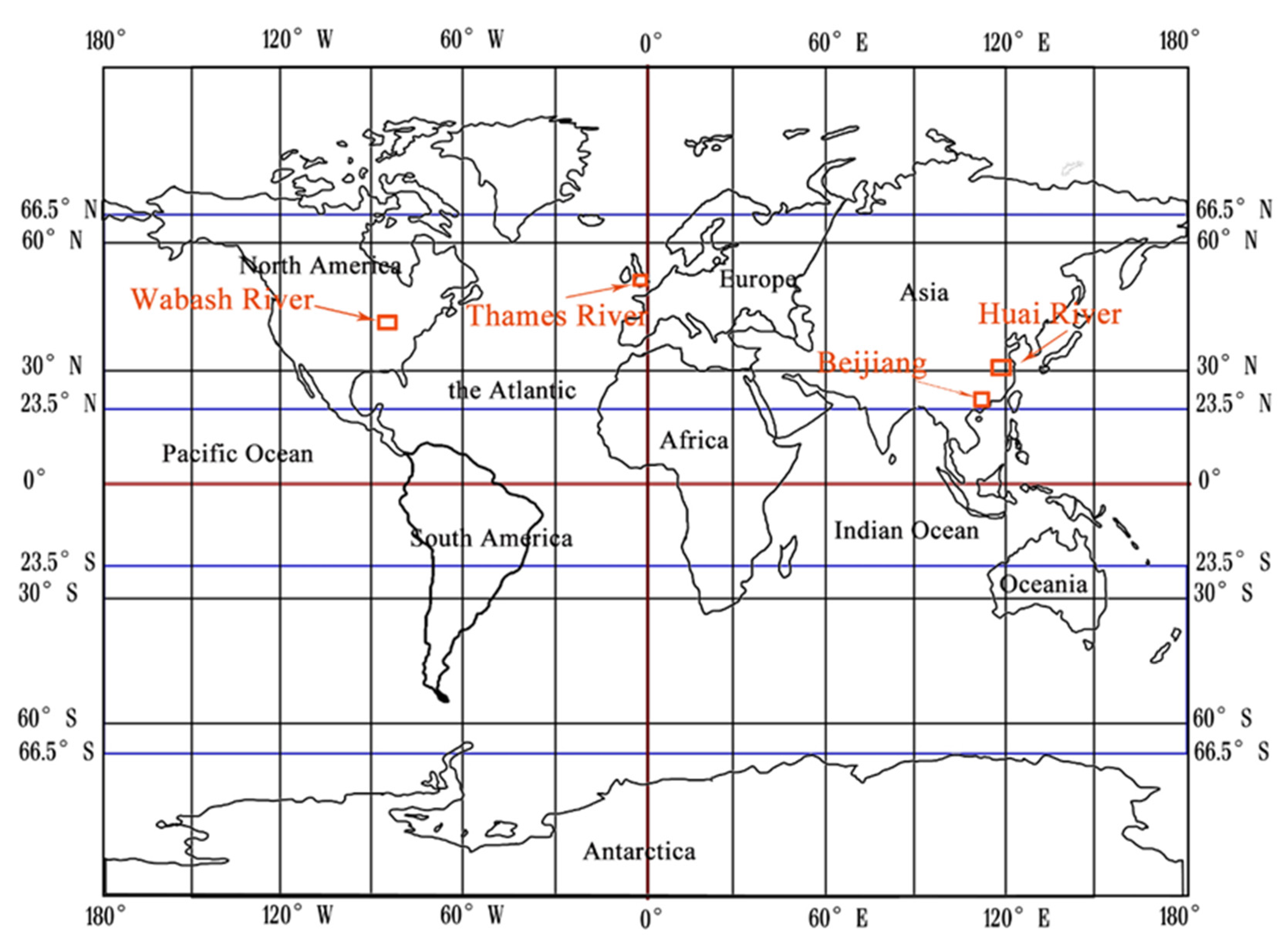
In order to verify the applicability of the methodology in different regions around the world, four hydrological stations with long historical data are used as case studies, including Kingston at Thames River, Lafayette at Wabash River, Shijiao at Beijiang River and Lutaizi at Huai River. These four stations are located in different areas in 23.5–66.5 degrees north of latitude in China, the UK and the US respectively (see Figure 1 and Table 2) with long-term data ranging from 48 to 127 years. Figure 1 gives their geographical locations and Table 2 summarizes the geographical and data information. The stations cover a wide range of climate conditions. Annual maximum daily flows are used in the analysis.
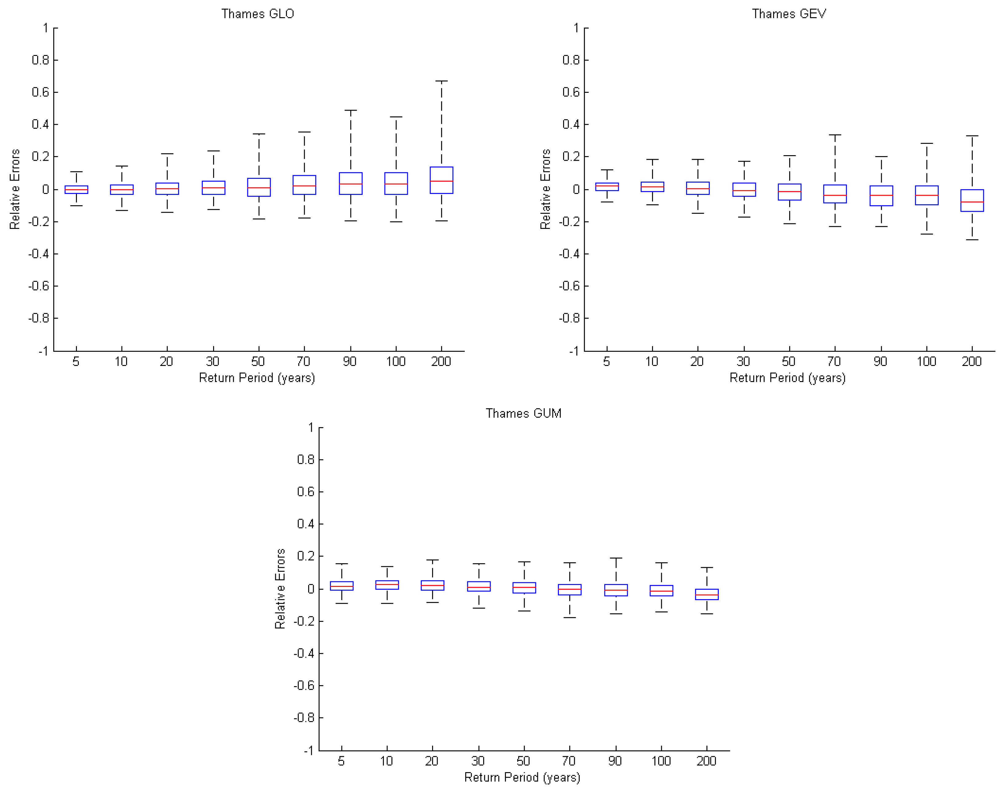
Thames River is the biggest river in the UK with the length of 338 km and drainage area of 9948 km2. It is located at a temperate climate zone with high humidity and relatively stable temperature. Kingston station, located at the lower reach of Thames River, is used in the study. The skewness coefficient Cs of the flood series at Kingston station is large with the value of 1.181, which implies a steep upper tail of the optimal frequency distribution.
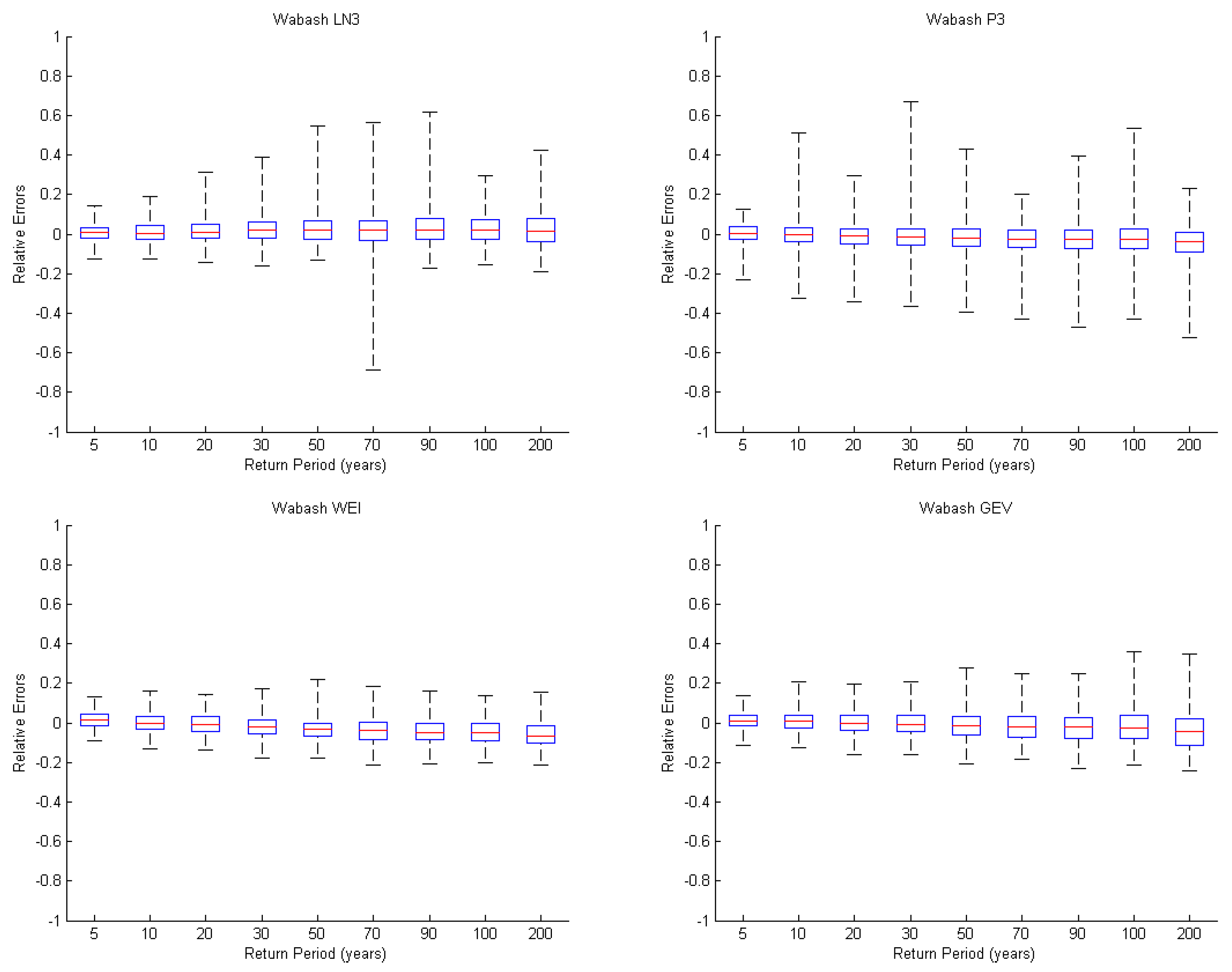
With a length of 810 km, Wabash River is the largest and most important river in Indiana, USA. Wabash basin, mostly in Indiana, is dominated by a humid continental climate with cold winters, and warm and wet summers. Lafayette station, which is located at the middle reach of Wabash River and controls a drainage area of 18,821 km2, is used in the study. The small Cs value of 0.280 for the flood series at Lafayette station indicates that the upper tail of the optimal frequency distributions is gentle at this station.
Beijiang River, located at the subtropical monsoon climate zone of China, has an annual average temperature between 14 and 22 °C, and an annual mean rainfall of 1700 mm. Shijiao station, the main controlling station (controlling a drainage area of 38,363 km2) located at the lower reach of the Beijiang River, is used in this study. The small Cs value of 0.230 for the flood series at Shijiao station shows a gentle upper tail frequency distribution at this station.
Huai River, located between Changjiang River (Yangtze River) and Huanghe River (Yellow River), covers a large area. Its north part is in a warm temperate zone, while the south part is in a monsoon climate zone with an annual average temperature between 11 and 16 °C. Lutaizi station, the control station in the middle river reach with a drainage area of 91,620 km2, is selected as a case study in this paper. For Lutaizi Station, the large Cs value of 1.198 infers a steep upper tail frequency distribution.
The record lengths of the data are given in Table 2 in descending order. The observed flood discharge series at each station is visually investigated to see if there are apparent trends or jumps. Statistical tests including the Spearman test for trend and the R/S analysis method for change point are conducted formally and summarized in 
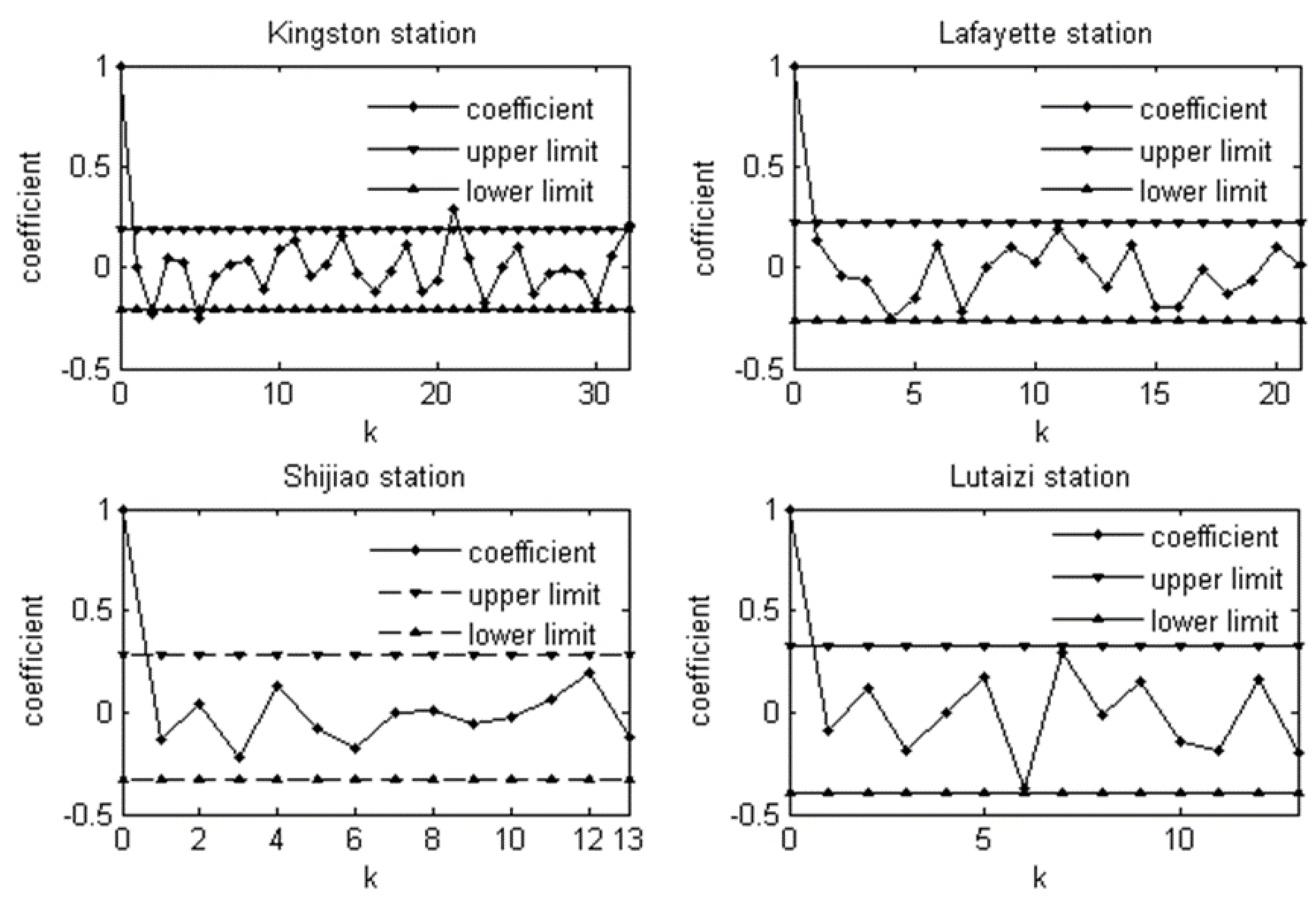
Table 3, from which it can be seen that there are no statistically significant trends and change point for annual maximum daily discharges. The fluctuation change of annual maximum flow is the biggest at Lafayette station and is the lowest at Kingston station. The autocorrelation coefficient and randomness test indicate that hydrological sequences satisfy the independent assumption (Figure 2). Therefore, the flood series data of the studied rivers fulfil the basic assumptions of traditional frequency analysis methods, i.e., stationary, independent and identically distributed over time.

4. Results and Discussions

The MLE method is conducted for parameter estimation of all eight distributions (P3, GLO, GEV, Weibull, Gumbel, LN3, LN2 and LP3), and the results are given in Table 4 with the associated return levels being plotted in Figure 3. The values of hypothesis tests and information-based criteria are summarized in Table 5, in which the smaller value for the test statistics means a better fitting by that test.

4.1. Optimal Frequency Distribution for Different Model Selection Methods

There are different selections of frequency distributions by using hypothesis tests and information-based criteria approaches for each river. Taking Thames River as an example, for the hypothesis tests KS and AD, the comparison results indicate that the data are best fitted by GLO distribution, followed by GEV and Gumbel distributions (Table 5). When information-based criteria methods (including AIC, AICc and BIC) are used in the comparison, results show that Gumbel fits the observed floods best, followed by GLO distribution (see Table 5; Figure 3). Some different results can be found between hypothesis tests and information-based criteria methods. Heavy tailed GLO distribution is the best fitted frequency distribution by the hypothesis tests, while mixed tailed Gumbel distribution is the best by the information-based criteria in Thames River.
As is the case for Thames River, the best fitted flood frequency distributions in Wabash River vary slightly between two types of model selection methods. Mixed tailed LN3 distribution is the best fitted frequency distribution for hypothesis tests, while light tailed Weibull distribution is the best for information-based criteria (Table 5).
There is always a difference between the two types of selection methods in the other two river basins. In Huai River, light tailed (P3, Weibull) distributions are suitable frequency distributions for hypothesis tests, while mixed tailed (LN2) or light tailed (Weibull) distributions are the best for information-based criteria (Table 5). In Beijiang River, light tailed (Weibull, P3) and mixed tailed (GEV) distributions are suitable frequency distributions for hypothesis tests, while mixed tailed (GEV) and light tailed (Weibull) distributions are the best for information-based criteria. The results show that the optimal flood frequency distributions are basically the same in both rivers although slightly different orders exist in Beijiang River. The study points out that in Beijiang River there is a slight tendency towards the selection of light tailed distributions, while heavy tailed distributions are inappropriate (Table 5).

4.2. Composite Criterion for Model Selection

For Thames River, the composite criterion of R M S E ¯ and Box plots of REs can correctly recognize, in most of the cases, that the optimal distribution belongs to the Gumbel. Information-based criteria turn out to be the best methods in this case, even with varying return periods (Table 6 and Figure 4). The Cs values have a close relationship with the optimal frequency distributions (Figure 3), the large Cs value of 1.181 for the flood series at Kingston station agrees with the selection of mixed tail distribution Gumbel as the optimal distribution.
As is the case for Thames River, information-based criteria are shown to be the best methods in Wabash River, even with varying return periods (Table 6 and Figure 5). It is found that Weibull can be judged as a suitable flood frequency distribution, which fits high flows well and is insensitive to low flows. For Lafayette station, the smaller Cs value of 0.280 is reflected by the selection of light tail Weibull distribution. There is a slight tendency towards the selection of light tailed distributions in Wabash River.
However, hypothesis tests appear to be the best methods in Beijiang River, even with varying return periods (Table 6 and Figure 6). In this river basin, Weibull is inferred as the suitable flood frequency distribution based on the composite criterion of R M S E ¯ and Box plots of REs. The smallest Cs value of 0.230 for Shijiao station is consistent with the selection of light tail Weibull distribution.
It should be noted that hypothesis tests and information-based criteria methods all give unsatisfactory performance in Huai River (Table 6 and Figure 7); Weibull can be viewed as the preferable flood frequency distribution in Huai River by the results of composite criterion. Its large Cs value of 1.198 is not consistent with the selection of light tail Weibull distribution, mainly because the influence of the extremely large flood in 1954.

4.3. Comparison on Hypothesis Tests and Information-Based Criteria for Upper Tail

The objective of this section is to verify whether the hypothesis tests and information-based criteria work correctly for the upper tail of flood frequency distributions and to analyse the cause and the mechanism when they are applied to identify the PDs of hydrological extremes.

4.3.1. Characteristics of Statistical Hypothesis Test

(1) Kolmogorov–Smirnov (KS)

The KS test measures the greatest discrepancy between the observed and hypothesized distributions which locate at the upper tail or lower tail of the distribution. So the optimal PDs selected by KS are different from the ones selected by a composite criterion when the greatest discrepancy locates at the lower tail. The optimal PD selected by KS is not suitable for fitting high flow. For example, although the values of the KS test for GLO PD in Thames River, LN3 PD in Wabash River, and GLO PD in Huai River are considerably smaller than that of all the other PDs, these particular models overestimate or underestimate the upper tail events a great number of times. Furthermore, these particular distributions always have a rather wide spread of REs, with R M S E ¯ value appreciably large (see Figure 4, Figure 5, Figure 7 and Table 6).

(2) Anderson–Darling Criterion (AD)

AD uses the sum of the squared differences between the empirical and theoretical distributions with weights to emphasize discrepancies in the tails. AD not only focuses on high flow end, but also addresses low flow end. Similar to KS, the optimal PD selected by AD is different from the one selected by a composite criterion when the emphasis is on the discrepancies located at the lower tail. For example, although the values of the AD test for GLO PD in Thames River and GLO PD in Wabash River are considerably smaller than that of all the other PDs, these models overestimate the upper tail events a greater number of times. Furthermore, these distributions always have a rather wide spread of REs, with R M S E ¯ value appreciably large (Figure 4 and Figure 5; Table 6). The optimal PDs selected by AD are never suitable for fitting high flows. In contrast, although GLO and LN3 do not perform so well at high flows, they fit the data well at the lower tail of the distribution, and these PDs are selected by AD in Wabash River as a final selection.

(3) Characteristics Summary

The statistical hypothesis tests (KS and AD) do not show rigorous results when focusing on the goodness of predictions of the extreme upper tail events. Although the values of the composite criterion for Gumbel PD in Thames River and Weibull PD in Wabash River show the best fitted distributions, the fitted order of Gumbel PD by KS and AD tests in Thames River is in the third place, and Weibull PD in Wabash River ranks fifth. Weibull PD selected by the composite criterion in Huai river ranks second by KS and AD. The results confirm some findings recently presented in the scientific literature. Laio et al. (2009) indicated that the statistical hypothesis testing methods have some evident limitations, because the obtained results are subjective, depending, for example, on the significance level chosen, and ambiguous, as often more than one distribution passes the goodness-of-fit tests [5].

4.3.2. Characteristics of Information-Based Criteria

(1) AIC, AICc Criteria

The optimal distributions selected by AIC and AICc are basically the same, and perform consistently with the distributions selected by the composite criterion. Although there are some differences in the values of AIC and AICc criteria for GEV PD in Beijiang River, they are considerably smaller than that of all the other PDs. However, these models overestimate the upper tail events when the return periods are greater than 70 years and underestimate the upper tail events for other return periods occasionally. The LN2 PD is selected by the AICc criterion in Huai River, however, LN2 PD sometimes overestimates the upper tail events and always has a rather wide range of REs, and with large R M S E ¯ values (Figure 6 and Table 6).

(2) BIC Criterion

BIC is a Bayesian version of the AIC which incorporates some information about the prior distribution of the parameters of the model. BIC penalizes heavier than AIC and AICc for the number of estimated parameters P and small sample sizes [11]. So it is easier to select a distribution with fewer parameters, such as LN2 and Gumbel for the same sequence length. This is why the optimal distribution (LN2) selected by BIC does not perform consistently with the Weibull PD selected by the composite criterion. LN2 PD often overestimates the upper tail events (Figure 7). In addition, the BIC criterion often prefers the LN2 PD to AIC and AICc in Huai River, Thames River and Beijiang River, and prefers the Gumbel PD to AIC and AICc in Beijiang River and Huai River.

(3) Characteristics Summary

The optimal frequency distributions selected by AIC, BIC and AICc are basically the same as the distributions selected by the composite criterion. The information-based criteria are more sensitive to the high flow than hypothesis tests. BIC and AICc have a slight tendency towards the selection of two-parameter distributions. These results are due to the characteristics in penalizing for the number of estimated parameters P, by which BIC and AICc penalize heavier than AIC for small sample sizes. This is the reason that the optimal distribution (LN2) selected by information-based criteria does not perform consistently with the distribution selected by composite criterion (Weibull) in Huai River. This result confirms some findings recently presented in the scientific literature such as Baldassarre (2009) [12]. The capability of the information-based criteria to recognize the correct parent distribution from available data samples varies from case to case; it is rather good in some cases, in particular when the parent is a two-parameter distribution [5].
In general, the information-based criteria perform better than hypothesis tests when the focus is on the goodness of predictions of the extreme upper tail events. Although the order is not always ranked first for the best fitted distributions selected by the composite criterion, these distributions all can be identified correctly by AIC, BIC and AICc in all the four rivers. Furthermore, these particular distributions selected by information-based criteria always have a rather narrow spread of REs, with small R M S E ¯ value. In contrast, the optimal frequency distributions for KS and AD are basically not the same as the distribution selected by the composite criterion. The reasons that information-based criteria are more sensitive to the high flow than hypothesis tests are as follows. The KS and AD criteria compare the distance of the flood point between theoretical and empirical frequencies. The closer the distance between the two, the better the model fitting degree. For the measured flood samples, small- and medium-level floods occur more frequently than big floods; the data for big floods at the upper tail of flood frequency distribution are scarce. Therefore, KS and AD may choose the distributions which focus on small- and medium-level floods (especially for the three-parameter distributions, because the fitting multi-parameter model can theoretically achieve good effect). This is different from the principle of information-based criteria, which do not compare the data distance between theoretical and empirical flood frequencies (distributions were selected on the basis of maximum likelihood values). Besides, information-based criteria can avoid over fitting and ensure the selection of the distribution which has a good epitaxial predictability by penalizing the model complexity. Furthermore, the value of the log-likelihood function can also reflect the goodness-of-fit of the probability model to observed points. The optimal distributions selected respectively by the KS and AD are often different. This can be easily seen from the results in Table 7 for Wabash River and Huai River. In contrast, the optimal frequency distributions selected respectively by AIC, BIC and AICc are basically the same. It is generally believed that AIC, BIC, AICc are stable for high flow in different rivers. In order to decide whether a particular distribution fits the high flow, it would be better to use the composite criterion which has the strongest applicability, followed by information-based criteria. The applicability of hypothesis tests is poor.

5. Conclusions

In this study, eight probability distributions have been used for flood frequency analysis in four selected rivers with different climatic conditions, and their goodness-of-fit has been examined by various statistical methods. By applying all the distributions with different selection criteria for comparison to a composite criterion, the following conclusions are drawn.
(1)
There are different selections of frequency distributions in the four rivers by using hypothesis tests and information-based criteria approaches. Hypothesis tests are more likely to choose complex, parametric models, and information-based criteria prefer to choose simple, effective models. Different selection criteria have no particular tendency toward the tail of the distribution.
(2)
The information-based criteria perform better than hypothesis test methods most of the time when focusing on the goodness of predictions of the extreme upper tails of PDs. The distributions selected by information-based criteria are more likely to be close to true values than the distributions selected by hypothesis test methods in the upper tail of the frequency curve.
(3)
The composite criterion not only can select the optimal distribution, but also can evaluate the error of the estimated value. In order to decide on a particular distribution to fit the high flow, it would be better to use the composite criterion.

Acknowledgments

The research is financially supported by the National Natural Science Foundation of China (Grant No.51210013, 51569009, 51479216, 51509127), the National Science and Technology Support Program (Grant No 2012BAC21B0103), the project from Natural science foundation of Hainan (414192, 20164157), the Public Welfare Project of Ministry of Water Resources (Grant No201401048). We also thank two anonymous referees for their valuable comments which helped the improvement of the manuscript.

Author Contributions

Xiaohong Chen designed the content and ideas of the research. Quanxi Shao and Chong-Yu Xu revised and improved the quality of the research, Jiaming Zhang, Lijuan Zhang and Changqing Ye calculated the data, Changqing Ye analysed the results. All authors reviewed the manuscript.

Conflicts of Interest

The authors declare no conflict of interest.

References

  1. Hussain, Z.; Pasha, G.R. Regional flood frequency analysis of the seven sites of Punjab, Pakistan, using L-Moments. Water Resour. Manag. 2009, 23, 1917–1933. [Google Scholar] [CrossRef]
  2. Chérif, R.; Bargaoui, Z. Regionalisation of Maximum Annual Runoff Using Hierarchical and Trellis Methods with Topographic Information. Water Resour Manag. 2013, 27, 2947–2963. [Google Scholar] [CrossRef]
  3. Faulkner, D.; Keef, C.; Martin, J. Setting design inflows to hydrodynamic flood models using a dependence model. Hydrol. Res. 2012, 43, 663–674. [Google Scholar] [CrossRef]
  4. Xia, J. Identification of a constrained nonlinear hydrological system described by Volterra Functional Series. Water Resour. Res. 1991, 27, 2415–2420. [Google Scholar]
  5. Laio, F.; Baldassarre, D.G.; Montanari, A. Model selection techniques for the frequency analysis of hydrological extremes. Water Resour. Res. 2009, 45. [Google Scholar] [CrossRef]
  6. Gomes, O.; Combes, C.; Dussauchoy, A. Parameter estimation of the generalized gamma distribution. Math. Comput. Simul. 2008, 79, 955–963. [Google Scholar] [CrossRef]
  7. Cicioni, G.; Guiliano, G.; Spaziani, F.M. Best fitting of probability functions to a set of data for flood studies. In Proceedings of the 2nd International Symposium on Hydrology of Floods and Droughts, Fort Collins, CO, USA, 11–13 September 1972; Water Resource Publication: Fort Collins, CO, USA, 1973; pp. 304–314. [Google Scholar]
  8. Akaike, H. Information theory and an extension of the maximum likelihood principle. Proceeding of the International Symposium on Information Theory, Budapest, Hungary, 2–8 September 1971; Peter, B.N., Csaki, F., Eds.; Akademiai Kiado: Budapest, Hungary, 1973; pp. 267–281. [Google Scholar]
  9. Hosking, J.R.M.; Wallis, J.R. The Value of Historical Data in Flood Frequency Analysis. Water Resour. Res. 1986, 22, 1606–1612. [Google Scholar] [CrossRef]
  10. Haktanir, T.; Horlacher, H.B. Evaluation of various distributions for flood frequency analysis. Hydrol. Sci. J. 1993, 38, 15–32. [Google Scholar] [CrossRef]
  11. Haddad, K.; Rahman, A.; Stedinger, J.J.R. Regional flood frequency analysis using Bayesian generalized least squares: A comparison between quantile and parameter regression techniques. Hydrol. Process. 2012, 26, 1008–1021. [Google Scholar] [CrossRef]
  12. Baldassarre, G.D.; Laio, F.; Montanaric, A. Design flood estimation using model selection criteria. Phys. Chem. Earth 2009, 34, 606–611. [Google Scholar] [CrossRef]
  13. Calenda, G.; Mancini, C.P.; Volpi, E. Selection of the probabilistic model of extreme floods: The case of the River Tiber in Rome. J. Hydrol. 2009, 371, 1–11. [Google Scholar] [CrossRef]
  14. Burnham, K.P.; Anderson, D.R. Model Selection and Multimodal Inference: A Practical Information-Theoretic Information-Theoretic Approach, 2nd ed.; Springer-Verlag: New York, NY, USA, 2002. [Google Scholar]
  15. Önöz, B.; Bayazit, M. Best-fit distributions of largest available flood samples. J. Hydrol. 1995, 167, 195–208. [Google Scholar] [CrossRef]
  16. House, P.K.; Baker, V.R. Paleohydrology of flash floods in small desert watersheds in western Arizona. Water Resour. Res. 2001, 37, 1825–1839. [Google Scholar] [CrossRef]
  17. Hosking, J.R.M.; Wallis, J.R. Paleoflood Hydrology and Flood Frequency Analysis. Water Resour. Res. 1986, 22, 543–550. [Google Scholar] [CrossRef]
  18. Luo, P.P.; He, B.; Takara, K.; APIP; Nover, D.; Kobayashi, K.; Yamashiki, Y. Paleo-hydrology and Paleo-flow Reconstruction in the Yodo River Basin. Annu. Disas. Prev. Res. Inst. Kyoto Univ. 2011, 54, 119–128. [Google Scholar]
  19. Begueria, S.; Angulo-Martinez, M.; Vicente-Serrano, S.M.; Lopez-Moreno, J.I.; El-Kenawy, A. Assessing trends in extreme precipitation events intensity and magnitude using non-stationary peaks-over-threshold analysis: A case study in northeast Spain from 1930 to 2006. Int. J. Climatol. 2011, 31, 2102–2114. [Google Scholar] [CrossRef]
  20. Magilligan, F.J.; Nislow, K.H. Changes in hydrologic regimes by dams. Geomorphology 2005, 71, 61–78. [Google Scholar] [CrossRef]
  21. Salas, J.D.; Obeysekera, J. Revisiting the concepts of return period and risk for nonstationary hydrologic extreme events. J. Hydrol. Eng. 2014, 19, 554–568. [Google Scholar] [CrossRef]
  22. Milly, P.C.D.; Betancourt, J.B.; Falkenmark, M.; Hirsch, R.M.; Kundzewicz, Z.W.; Lettenmaier, D.P.; Stouffer, R.J. Stationarity is dead: Whither water management? Science 2008, 319, 2. [Google Scholar] [CrossRef] [PubMed]
  23. Khaliq, M.N.; Ouarda, T.B.M.J.; Ondo, J.C.; Gachon, P.; Bobée, B. Frequency analysis of a sequence of dependent and/or non-stationary hydro-meteorological observations: A review. J. Hydrol. 2006, 329, 534–552. [Google Scholar] [CrossRef]
  24. Chen, X.H.; Zhang, L.J.; Xu, C.-Y.; Zhang, J.M.; Ye, C.Q. Hydrological design of non-stationary flood extremes and durations in Wujiang river, South China: Changing properties, causes and impacts. Math. Probl. Eng. 2013, 2013. [Google Scholar] [CrossRef]
  25. Yan, L.; Xiong, L.H.; Liu, D.D.; Hu, T.S.; Xu, C.-Y. Frequency analysis of nonstationary annual maximum flood series using the time-varying two-component mixture distributions. Hydrol. Process. 2017, 31, 69–89. [Google Scholar] [CrossRef]
  26. Rao, A.R.; Hamed, K.H. Flood Frequency Analysis; CRC Press: Boca Raton, FL, USA, 2000; pp. 10–12. [Google Scholar]
  27. Reiss, R.-D.; Thomas, M. Statistical Analysis of Extreme Values: With Applications to Insurance, Finance, Hydrology and Other Fields; Birkäuser: Basel, Switzerland, 2001; pp. 49–50. [Google Scholar]
  28. El Adlouni, S.; Bobée, B.; Ouarda, T.B.M.J. On the tails of extreme event distributions in hydrology. J. Hydrol. 2008, 355, 16–33. [Google Scholar] [CrossRef]
  29. Reis, D.D.S.; Stedinger, J.J.R. Bayesian MCMC flood frequency analysis with historical information. J. Hydrol. 2005, 313, 97–116. [Google Scholar] [CrossRef]
  30. Huang, W.R.; Xu, S.D.; Nnaji, S. Evaluation of GEV model for frequency analysis of annual maximum water levels in the coast of United States. Ocean Eng. 2008, 35, 1132–1147. [Google Scholar] [CrossRef]
  31. Martins, E.S.; Stedinger, J.R. Generalized maximum-likelihood generalized extreme-value quantile estimators for hydrologic data. Water Resour. Res. 2000, 36, 737–744. [Google Scholar] [CrossRef]
  32. Hirose, H. Maximum likelihood estimation in the 3-parameter Weibull distribution: A look through the generalized extreme-value. IEEE Trans. Dielectr. Electr. Insul. 1996, 3, 43–55. [Google Scholar] [CrossRef]
  33. Otten, A.; Montfort, V. Maximum-likelihood estimation of the general extreme-value distribution parameters. J. Hydrol. 1980, 47, 187–192. [Google Scholar] [CrossRef]
  34. Yevjevich, V. Probability and Statistics in Hydrology; Water Resources Publications: Fort Collins, CO, USA, 1972; pp. 214–232. [Google Scholar]
  35. Ben-Zvi, A. Rainfall intensity–duration–frequency relationships derived from large partial duration series. J. Hydrol. 2009, 367, 104–114. [Google Scholar] [CrossRef]
  36. Laio, F. Cramer-von Mises and Anderson-Darling goodness of fit tests for extreme value distributions with unknown parameters. Water Resour. Res. 2004, 40, W09308. [Google Scholar] [CrossRef]
  37. Burnham, K.P.; Anderson, D.R. Multimodel Inference: Understanding AIC and BIC in model selection. Sociol. Methods Res. 2004, 33, 261–304. [Google Scholar] [CrossRef]
  38. Moriasi, D.N.; Arnold, J.G.; Van Liew, M.W.; Bingner, R.L.; Harmel, R.D.; Veith, T.L. Model evaluation guidelines for systematic quantification of accuracy in watershed simulations. Trans. Asabe, 2007, 50, 885–900. [Google Scholar] [CrossRef]
  39. Hosking, J.R.M.; Wallis, J.R. Regional Frequency Analysis: An Approach Based on L-moments; Cambridge University Press: Cambridge, UK, 1997; pp. 19–20. [Google Scholar]
  40. Xie, P.; Lei, H.F.; Chen, G.C.; Li, J. A Spatial and Temporal Variation Analysis Method of Watershed Rainfall Based on Hurst Coefficient. J. China hydrol. 2008, 28, 6–10. [Google Scholar]
  41. Wallis, J.R.; Matalas, N.C. Small sample properties of H and K—Estimations of the Hurst coefficient h. Water Resour. Res. 1970, 6, 1583–1594. [Google Scholar] [CrossRef]
Figure 1. The locations of the studied stations.
Water 09 00320 g001
Figure 2. Autocorrelation coefficient for annual maximum daily flows in the four rivers.
Water 09 00320 g002
Figure 3. A comparison of the eight typical frequency distributions for four rivers with parameters estimated by MLE. (a) Thames River; (b) Wabash River; (c) Beijiang River and (d) Huai River.
Water 09 00320 g003
Figure 4. Box plots of the relative errors (REs) of the Kingston at Thames River for sample series length 127, with Kappa as the parent probability distribution (PD).
Water 09 00320 g004
Figure 5. Box plots of the relative errors (REs) of the Lafayette at Wabash River for sample series length 85, with Kappa as the parent PD.
Water 09 00320 g005
Figure 6. Box plots of the relative errors (REs) of the Shijiao at Beijiang River for sample series length 53, with Kappa as the parent PD.
Water 09 00320 g006
Figure 7. Box plots of the relative errors (REs) of the Lutaizi at Huai River for sample series length 48, with Kappa as the parent PD.
Water 09 00320 g007
Table 1. Model selection criteria methods for hydrological frequency analysis.
Goodness-of-Fit Test (GOFT)Statistic ValueDescriptionCharacteristic
KS D n = max 1 i n [ i N F ( x ( i ) ) , F ( x ( i ) ) i 1 N ] [34] x ( i ) is a plot on the Empirical frequency curve and F−1(p) is the Inverse function of cumulative distribution function F(x) for probability P(i). N is the size of samples.KS test measures the greatest discrepancy between the observed and hypothesized distributions.
AD A 2 = N 1 N i = 1 N ( 2 i 1 ) [ ln F ( x ( 1 ) ) + ln { 1 F ( x ( N i + 1 ) ) } ] [35]AD uses the sum of the squared differences between the empirical and theoretical distributions with weights to emphasize discrepancies in the tails. AD Statistic has shown good capabilities for a small sample size and heavy tailed distributions [ 15,36].
AIC A I C = 2 ln [ L ( D | θ ) ] + 2 m [8] L ( D | θ ) is the likelihood function of a certain distribution with parameter set θ and data array D. m is the number of parameters P and n is the size of the sample.The log-likelihood maximised function value is used to select the model and penalize heavier for the number of estimated parameters P. In some situations where the sample size n is small with respect to the number of estimated parameters P, the AIC may perform inadequately [11]; a second-order variant of AIC, called AICc, should be used.
BIC B I C = 2 ln [ L ( D | θ ) ] + ln ( n ) m [37]Similar to the AIC, but developed in a Bayesian framework. BIC penalizes heavier than AIC for number of estimated parameters P and small sample sizes [11].
AICc A I C c = 2 ln [ L ( D | θ ) ] + 2 m ( n n m 1 ) [14]The AICc penalizes heavier than AIC for number of estimated parameters P and can be adopted when n/P <40 to reduce bias [13].
Table 2. Background information of the four study basins.
Basin and Station NameCountryArea (Km2)TerrainClimate ZoneData LengthCs of the Flood Series
Kingston at ThamesUK9948PlainTemperate1883–20091.181
Lafayette at WabashUSA18,821Alluvial PlainHumid Continental Climate1907–19910.280
Shijiao at BeijiangChina38,363HillSubtropical Monsoon1956–20080.230
Lutaizi at HuaiChina91,620HillWarm Temperate and Half Wet Monsoon Climate1951–19981.198
Table 3. Randomness test for annual maximum daily flows in the four rivers.
Study AreaSignificancePersistencyTrendJump
tSpearmanHurst Coefficient
Kingston at ThamesStats0.0571.4460.568
Critical Value (5%)1.9791.960.628
Accept or Notyesyesyes
Lafayette at WabashStats1.286−0.4530.491
Critical Value (5%)1.9891.960.323
Accept or Notyesyesyes
Shijiao at BeijiangStats−0.9530.9270.500
Critical Value (5%)2.0081.960.674
Accept or Notyesyesyes
Lutaizi at HuaiStats−0.534−0.9250.435
Critical Value (5%)2.0141.960.255
Accept or Notyesyesyes
Table 4. Parameter estimation for annual maximum daily flows in the four rivers.
Study AreaPDsParameters (MLE)
ScaleShapeLocation
Kingston at ThamesP30.0278.5115.31
GLO56.67−0.16310.86
GEV89.0590.036278.97
Weibull282.292.3676.12
Gumbel88.47——277.22
LN30.265.94−69.57
LN20.335.73——
LP339.104171.621.34
Lafayette at WabashP30.01132.36−1644.73
GLO299.93−0.0651365.28
GEV506.810.2031185.48
Weibull1433.112.56117.46
Gumbel490.76——1133.93
LN30.128.41−3140.96
LN20.457.15——
LP328.22171.621.082
Shijiao at BeijiangP30.001936.96−9811.59
GLO1819.32−0.0689436.47
GEV3054.670.228325.95
Weibull8802.032.641782.32
Gumbel2912.39——8000.08
LN30.1110.26−19384.8
LN20.379.11——
LP334.13171.364.087
Lutaizi at HuaiP30.000551.89566.84
GLO1264.17−0.363480.44
GEV1671.23−0.122861.17
Weibull3676.231.39672.028
Gumbel1750.16——2942.83
LN30.438.47−1281.45
LN20.628.109——
LP320.55166.680.00001
Table 5. A comparison of the test statistic values of the eight typical frequency distributions for hypothesis tests and information-based criteria.
Study AreaFrequency DistributionsKSADAICBICAICc
Kingston at ThamesP30.0640.5021542.4191550.9511542.614
GLO0.0530.2921538.7281547.2601538.923
GEV0.0540.3551540.2121548.7451540.407
Weibull0.0891.3661552.0911560.6231552.286
Gumbel0.0550.3841538.7081544.3961538.804
LN30.0570.3891540.8011549.3341540.996
LN20.0560.3961540.2271545.9161540.324
LP30.0720.5321544.7001553.3001544.900
Lafayette at WabashP30.0600.4431313.1541320.4821313.450
GLO0.0700.3971314.5641321.8921314.860
GEV0.0630.4551312.9271320.2551313.224
Weibull0.0730.5631312.4741319.8021312.770
Gumbel0.0861.0401317.3431322.2281317.489
LN30.0600.4371313.1901320.5181313.487
LN20.1101.8491324.4461329.3321324.593
LP30.1142.1741331.1041338.4321331.401
Shijiao at BeijiangP30.1060.4361013.8541019.7641014.343
GLO0.1220.5731012.8761018.7871013.366
GEV0.0980.4241010.3211016.2321010.811
Weibull0.0960.4161010.5711016.4811011.060
Gumbel0.1090.6441012.4381016.3791012.678
LN30.1060.4391010.7531016.6641011.243
LN20.1140.7091014.0451017.9861014.285
LP30.1190.8671018.5471024.4581019.037
Lutaizi at HuaiP30.0770.181873.463879.077874.008
GLO0.0690.290876.908882.521877.453
GEV0.0850.255875.763881.377876.308
Weibull0.0700.188872.889878.503873.435
Gumbel0.0960.370874.770878.513875.037
LN30.0880.237875.352880.966875.898
LN20.0800.233873.109876.852873.376
LP30.0770.289875.939881.553876.485
Table 6. RMSE and R M S E ¯ calculated for different return periods T in the four rivers.
RiverPDT = 5T = 10T = 20T = 30T = 50T = 70T = 90T = 100T = 200 R M S E ¯
ThamesGUM0.0390.0440.0490.0470.0500.0480.0520.0520.0590.049
GLO0.0320.0420.0560.0660.0830.0940.1110.1140.1450.083
GEV0.0380.0450.0550.0630.0760.0880.0890.0930.1260.075
WabashLN30.0430.0500.0620.0670.0790.0920.0860.0790.0950.073
P30.0490.0660.0700.0810.0810.0880.0860.0950.1010.080
WEI0.0430.0460.0520.0580.0640.0750.0750.0760.0880.064
GEV0.0430.0480.0580.0640.0770.0770.0850.0900.1070.072
GLO0.0410.0450.0590.0680.0920.1100.1290.1360.1760.095
BeijiangWEI0.0460.0510.0610.0550.0570.0600.0630.0630.0640.058
GEV0.0480.0520.0590.0580.0690.0710.0780.0850.0960.068
P30.0550.0610.0850.0780.0800.0890.0890.0930.1140.083
HuaiWEI0.0990.1030.1140.1180.1260.1330.1450.1460.1460.126
P30.1030.1090.1360.1610.1690.1710.1900.1880.2160.160
LN20.0970.1070.1380.1660.2140.2450.2730.2940.3690.211
GLO0.1010.1320.2340.3310.4430.4680.5080.5000.5510.363
Table 7. The best fitted frequency distributions in the four rivers.
RiverHypothesis TestsInformation-Based CriteriaComposite Criterion
KSADKS, ADAverage Number of ParametersAICBICAICcAIC, BIC, AICcAverage Number of Parameters
Kingston at ThamesGLO, GEV, GUMGLO, GEV, GUMGlo, Gev (Heavy or Mixed)3GUM, GLO, GEVGUM, LN2, GLOGUM, GLO, LN2Gum, Glo (Mixed or Heavy)2.5Gum (Mixed)
Lafayette at WabashLN3, P3, GEVGLO, LN3, P3Ln3, P3 (Mixed or Light)3WEI, GEV, P3WEI, GEV, P3WEI, GEV, P3Wei, Gev (Light or Mixed)3Wei (Light)
Shijiao at BeijiangWEI, GEV, P3WEI, GEV, P3Wei, Gev (Light or Mixed)3GEV, WEI, P3GEV, GUM, WEIGEV, WEI, LN3Gev, Wei (Mixed or Light)3Wei (Light)
Lutaizi at HuaiGLO, WEI, P3P3, WEI, LN2P3, Wei (Light)3WEI, LN2, P3LN2, WEI, GUMLN2, WEI, P3Ln2, Wei (Mixed or Light)2.5Wei (Light)

