
A Semi-Infinite Interval-Stochastic Risk Management Model for River Water Pollution Control under Uncertainty

1
Department of Environmental Engineering, Xiamen University of Technology, Xiamen 361024, China
2
Institute for Energy, Environment and Sustainable Communities, University of Regina, Regina, SK S4S 0A2, Canada
*
Author to whom correspondence should be addressed.
Water 2017, 9(5), 351; https://doi.org/10.3390/w9050351
Submission received: 14 March 2017
/
Revised: 20 April 2017
/
Accepted: 12 May 2017
/
Published: 18 May 2017
(This article belongs to the Special Issue Modeling of Water Systems)
Abstract
:In this study, a semi-infinite interval-stochastic risk management (SIRM) model is developed for river water pollution control, where various policy scenarios are explored in response to economic penalties due to randomness and functional intervals. SIRM can also control the variability of the recourse cost as well as capture the notion of risk in stochastic programming. Then, the SIRM model is applied to water pollution control of the Xiangxihe watershed. Tradeoffs between risks and benefits are evaluated, indicating any change in the targeted benefit and risk level would yield varied expected benefits. Results disclose that the uncertainty of system components and risk preference of decision makers have significant effects on the watershed's production generation pattern and pollutant control schemes as well as system benefit. Decision makers with risk-aversive attitude would accept a lower system benefit (with lower production level and pollutant discharge); a policy based on risk-neutral attitude would lead to a higher system benefit (with higher production level and pollutant discharge). The findings can facilitate the decision makers in identifying desired product generation plans in association with financial risk minimization and pollution mitigation.
1. Introduction
Currently, the problem of water quality deterioration (e.g., water pollution) hinders socio-economic development and eco-environmental sustainability in many countries (e.g., China). According to the 2015 China Water Resources Bulletin, approximate 19.7% of the monitored river water (i.e., the total length of monitored river is 235 × 103 km) is in the worst two categories of water quality classification system (i.e., no longer fishable and of questionable agricultural value) [1]. Effective planning of water pollution control for watersheds plays an important role for national and/or regional sustainable development [2,3,4]. In fact, decisions in water pollution control are often made on the basis of uncertain information (i.e., various uncertainties) existing in system components and their interactions [5,6]. The major sources of uncertainty in water pollution control are the random characteristics of natural processes (e.g., precipitation and climate change) and stream conditions (e.g., stream flow, water supply, and point/nonpoint source pollution), the errors in estimated modeling parameters, and the imprecision of system objectives and constraints [7]. For example, pollutant discharge allowances are often affected by pollutant discharge rates (which influenced by random events such as temperature and precipitation) and decision makers’ estimations; the allowable loads are not measured with certainty but in fact represent a probability distribution. Consequently, a number of mathematical techniques were launched to examine economic, environmental and ecological impacts of alternative pollution control actions under uncertainty, and thus aid the decision makers in generating effective water pollution control plans and policies [8,9,10,11,12,13,14,15,16,17].
Two-stage stochastic programming with recourse (TSP) is effective for problems where an analysis of policy scenarios is desired and uncertainties are expressed as random variables with known probability distributions [18,19]. The fundamental idea behind TSP is the concept of economic penalties with recourse that is the ability to take corrective actions after a random event occurs [20]. Previously, a number of researchers applied the TSP method to water pollution control [21]. Luo et al. [22] presented a simulation-based interval two-stage stochastic programming model for agricultural nonpoint source pollution control through land retirement under uncertain conditions, with the annual load of effluents before retirement being expressed as probability distributions. Harrison et al. [23] proposed a two-stage stochastic decision making programming method for problem of water quality pollution control. It was applicable to problems characterized by uncertainty in unobservable parameters; meanwhile, some problems were resolved upon observation of the outcome of the first-stage decision. Tavakoli [24] proposed a nonlinear two-stage stochastic fuzzy programming to tackle uncertainties described as fuzzy boundary intervals and probability distributions in decision making of optimal water allocation and pollutant load policies. Hu et al. [25] proposed a Bayesian-based two-stage inexact optimization method for supporting water pollution control under uncertainty; optimal production patterns of economic activities under different pollutant discharge allowance scenarios were generated. Generally, one major limitation of TSP is that it can only account for the expected second-stage cost without any consideration on the variability of the recourse values. For example, in water pollution control problems, one targeted benefit is firstly set, where one part is regular benefit from production generation and the other is in the case of excess pollutant discharge. If the event occurs, the penalty related to the pollutant mitigation might be tremendous such that the system benefit (i.e., the difference between the two parts) could be lower than the expected value. Although the event may happen associated with a low probability, it is unacceptable once it arises; any expected benefit below the targeted value is considered risky. The TSP model may become infeasible when the decision makers are risk averse under high variability conditions [26]. Ignoring risk might generate an unacceptable value for the objective function, which could lead to terrible outcomes for some extreme scenarios.
An effective tool that could help overcome the above shortcoming is financial risk management (i.e., risk below a certain targeted benefit), which was proposed to control the variability of the recourse cost, as well as capture the notion of risk in TSP [27,28]. The TSP model coupled with financial risk management enable decision makers to account for uncertainty in the evaluation and comparison of alternatives, while at the same time maximize the expected benefit and minimize the financial risk at every benefit level. Koppol and Bagajewicz [29] proposed a financial risk management based two-stage stochastic programming for the design of water utilization systems in process plants, where risk constraints were introduced to balance between cost and system reliability. Barbaro and Bagajewicz [30] presented a methodology which included financial risk management in the framework of two-stage stochastic programming for planning under uncertainty. Liu and Huang [31] proposed a dual interval two-stage restricted-recourse programming method to control the variability of the recourse cost of flood-diversion planning problem. Ahmed et al. [32] proposed financial risk management based two-stage stochastic programming for energy planning under uncertainties in demand and fuel price, in which the financial risk constraint were employed to choose the first stage decision in an optimal way without anticipation of future outcomes of uncertainties. Financial risk management is an advantageous measure to assess risk and obtain solutions appealing to decision makers. However, in practical water pollution control problems, various uncertain components may exist and may not be available as probability distribution and/or deterministic values, such as cost/benefit coefficients and pollutant discharge rates. Interval may be an appropriate format for dealing with uncertainties that cannot be quantified as distribution functions and/or deterministic values; moreover, the lower and upper bounds of interval numbers may be presented as functions instead of deterministic values when they vary with independent variables (e.g., time) [33]. Semi-infinite interval programming (SIP) can handle such dual uncertainties (i.e., functional intervals).
Therefore, this study aims at developing a semi-infinite interval-stochastic risk management (SIRM) model and applying it to water pollution control of the Xiangxihe watershed. The detailed tasks include: (i) integrating the concepts of financial risk management and functional interval parameters into a two-stage stochastic programming (TSP) framework, (ii) handling uncertainties presented as probability distributions and functional interval values, (iii) examining various scenarios that are related to economic penalties when the designed targets are violated, (iv) analyzing results of benefit, product generation and pollution control under a variety of risk levels, and (iv) assessing tradeoffs between risk and benefit on the basis of cumulative risk curves under different decision alternatives.
2. Methodology
Two-stage stochastic programming (TSP) reflects a tradeoff between pre-regulated strategies and the associated adaptive adjustments being approached to the expected system benefit [5]. In general, a TSP with recourse model can be formulated:
subject to:
where represent the first-stage decision variables, which have to be decided before the actual realizations of the random variables; denote the second-stage decision variables, which are related to the recourse actions against any infeasibilities due to particular realizations of uncertainties; is coefficient of the first-stage decision variable () in the objective function; is coefficient of the recourse variable () in the objective function; is coefficient of the first-stage decision variable () in constraint; is right-hand side parameter in constraint; is coefficient of in constraint j, which is associated with probability level . are random variables with probability levels , where h = 1, 2, …, v and . The objective function is composed of the benefit of first-stage decision minus the expected cost of the second stage under a series of constraints.
In water pollution control problems, when pollutant discharge is expressed as a random variable with known probability distribution, the actual benefit under pollutant discharge allowance scenarios may be unacceptably low, although the system expected benefit is maximized, due to the preceding TSP model’s incapability in providing any control over the variability of the benefit under each scenario (h). Such a risk of loss (or potential regret from the decision makers) may be due to the above modeling situations where the variability of the second-stage cost is not considered except for its expected value [34]. Therefore, a concept of financial risk is introduced into the TSP problems, which is defined as the probability of not meeting the targeted benefit (η) in each individual scenario realization [29,30]:
where is the actual benefit (i.e., the benefit resulting after the uncertainty has been unveiled and scenario h has been realized). For any scenario, the benefit is either greater or equal than the targeted value; the corresponding probability is zero (i.e., ), or the benefit of the scenario is smaller than the target, rendering a probability of 1 (i.e., ). In order to control the financial risk of one TSP problem, Equations (2) to (4) can be converted into:
where is the allowable risk exposure level. The integer variable should take a value of 1 if the benefit for scenario h is smaller than or equal to the targeted value () and a value of 0 otherwise. An upper-bound cost under each scenario (UBh) is used for balancing benefit for scenario h and the target level () [35].
In many real-world problems, some parameters may be presented as interval numbers; meanwhile, the lower and upper bounds of them can rarely be acquired as deterministic values. Instead, they may be presented as functions of independent variables; this leads to functional intervals. For example, decision makers may estimate that the pollutant discharge allowance may vary with time (t). Different time corresponds to different lower and upper bounds of pollutant discharge allowance (e.g., ), resulting in infinite pollutant discharge allowance values. Semi-infinite interval programming (SIP) can handle such dual uncertainties. Therefore, through introducing concepts of SIP and financial risk management into TSP model, a semi-infinite interval-stochastic risk management (SIRM) model can be formulated as follows:
subject to:
where superscripts ‘−’ and ‘+’ represent lower and upper bounds of the interval values; denotes pollutant discharge allowance that vary with time; denotes the length of time. In this study, a two-step solution process is proposed to transform the SIRM model into two deterministic submodels corresponding to the lower and upper bounds of the desired objective-function values. Figure 1 presents the overall flow chat of the methodology. The detailed solution method and procedure are presented in Appendix A to this paper.
3. Case Study
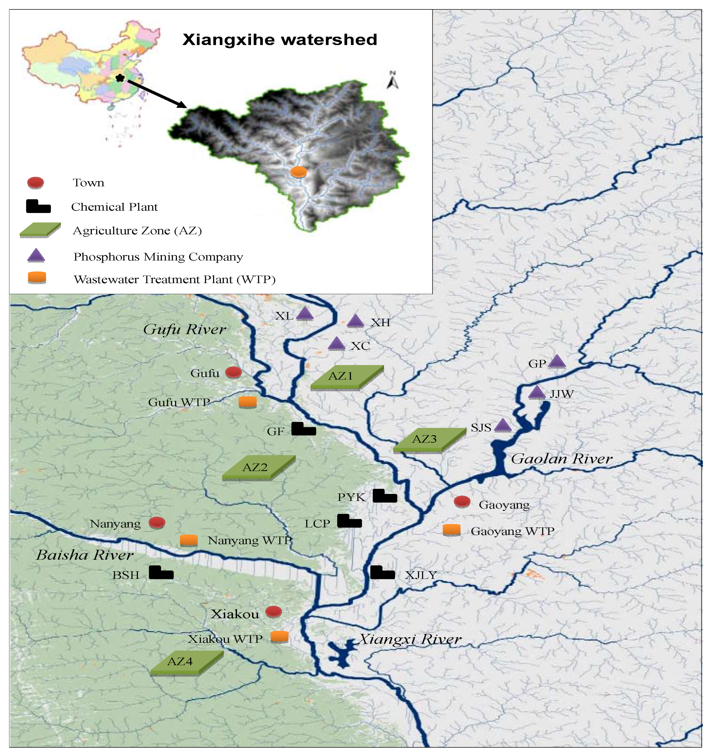
3.1. Study Area
Currently, water pollution problems due to point and nonpoint source pollution discharges have become more and more challenging in this watershed. Five chemical plants (i.e., GF, BSH, PYK, LCP, and XJLY), six phosphorus mining companies (i.e., XL, XH, XC, GP, JJW, and SJS), and four wastewater treatment plants (WTPs) (i.e., Gufu, Nanyang, Gaoyang, and Xiakou), four agricultural zones (AZ1 to AZ4) are the main pollutant discharge sources. These point and nonpoint sources scatter along a length of about 51 km river stretch which is segmented into five reaches (as shown in Figure 2). In the watershed, the main problems include: (1) the immoderate discharge of high-concentration phosphorus-containing wastewater and industrial soil wastes (i.e., chemical wastes, slags, and tailings) far exceed what can be decomposed by self-purification; (2) high potential for generating soil erosion and surface runoff due to the special geography and heavy rainfall; (3) large amounts of nutrient pollutants (in terms of phosphorus and nitrogen) in livestock wastewater and wastes are drained into the river by direct discharge or in rainfall. Effective water pollution control schemes are essential for the local sustainable development. In this study, a one-year planning horizon is selected and further sorted into two periods: dry season (i.e., November to May of the following year) and wet season (i.e., June to October) based on the specific growth periods of different crops. Wheat, potato, rapeseed, and alpine rice are identified as crops in dry season; second rice, maize, and vegetables are considered during wet season; citrus and tea grow up over the whole planning horizon.
3.2. Modelling Formulation
Then, the SIRM model is applied to optimize economic activities (i.e., industrial and agricultural activities) in the Xiangxihe watershed. The objective is to maximize the system benefit through identifying desired activities of chemical plants, phosphorus mining company, wastewater treatment plants, and crop farming. Biological oxygen demand (BOD), total nitrogen (TN) and total phosphorus (TP) are chosen as water quality indicators. The constraints involve relationships among economic activity, environmental restriction, and resources availability. The application of the proposed method is based on several assumptions: (1) the uncertainties, expressed as intervals and probability distributions, are independent; (2) the constraints are simplified with the respect to pollution loads rather than contaminant concentration, in order to prevent unnecessary complexity in the optimization procedure [36]. The SIRM model for supporting water pollution control in the Xiangxihe watershed can be represented as follows:
Constraints:
- (1)
- Wastewater treatment capacity constraints:
- (2)
- BOD discharge constraints:
- (3)
- Nitrogen discharge constraints:
- (4)
- Phosphorus discharge constraints:
- (5)
- Soil loss constraints:
- (6)
- Financial risk management:
- (7)
- Cropland resources constraints:
- (8)
- Industrial production scale constraints:
- (9)
- Non-negative constraints:
The detailed nomenclatures for variables and parameters are provided in Appendix B. In the above modeling formulation, pollutant discharge allowances are selected as the key constraints and expressed as probability distributions (which are divided into functional intervals).
3.3. Data Analysis
The imprecise inputs are investigated through field surveys, statistical yearbooks, government reports, and literatures. They are presented as functional intervals, probability distributions, and interval numbers. Table 1 displays net benefits and penalties from industrial activities (chemical plant, water supply, and phosphorus mining company) that presented as intervals. Given a production target that is promised to each industrial activity, if the target is determined too high, the excessive pollutants will have to be mitigated in a more expensive way or discharged/drained into the stream (leading to penalties from the government). Table 2 lists the pollutant discharge allowances for different industrial activities which are presented as probability distributions. They are divided into a set of discrete functional intervals with probability distributions to approximate the stochastic values since the amounts of pollutant discharge are vary during the day in each season. The pollutant discharge allowances are estimated by the decision makers to fall within reasonable ranges. In this study, it is assumed that the lengths of dry and wet seasons are 213 and 152 days, respectively. Five scenarios for pollutant discharge allowance are generated, which are named as low, low-medium, medium, medium-high, and high, respectively.
4. Results and Discussion
4.1. Benefit and Cost
In this study, a number of financial risk levels from 0 to 1 (ε) were taken into account. Figure 3 displays the results of various benefits (i.e., targeted benefit, system benefit, and regular benefit) and cost (i.e., penalty) under different risk levels. An increase in the targeted benefit implies the raised product generation meeting economic requirement in advance as the ε level is raised; an increase in the penalty for excessive pollutant discharge would then exist in case of low pollutant discharge allowance event occurring. In addition, any change in targeted benefit and ε level would lead to different system benefits; the trend of the variation along with the ε level would illustrate a balance between economic objective and violation risk. For instance, when ε = 0.12 (with = RMB¥ [100,600] × 106), the system benefit would be RMB¥ [121.9, 646.3] × 106; when ε = 0.64 (with = RMB¥ [160,800] × 106), the system benefit would be RMB¥ [160.8, 800.6] × 106. An increased ε level (a raised risk) corresponds to a decreased strictness for the constraints and thus an increased system benefit; such an increased value, however, would be associated with a raised constraint-violation risk.
4.2. Risk Analysis
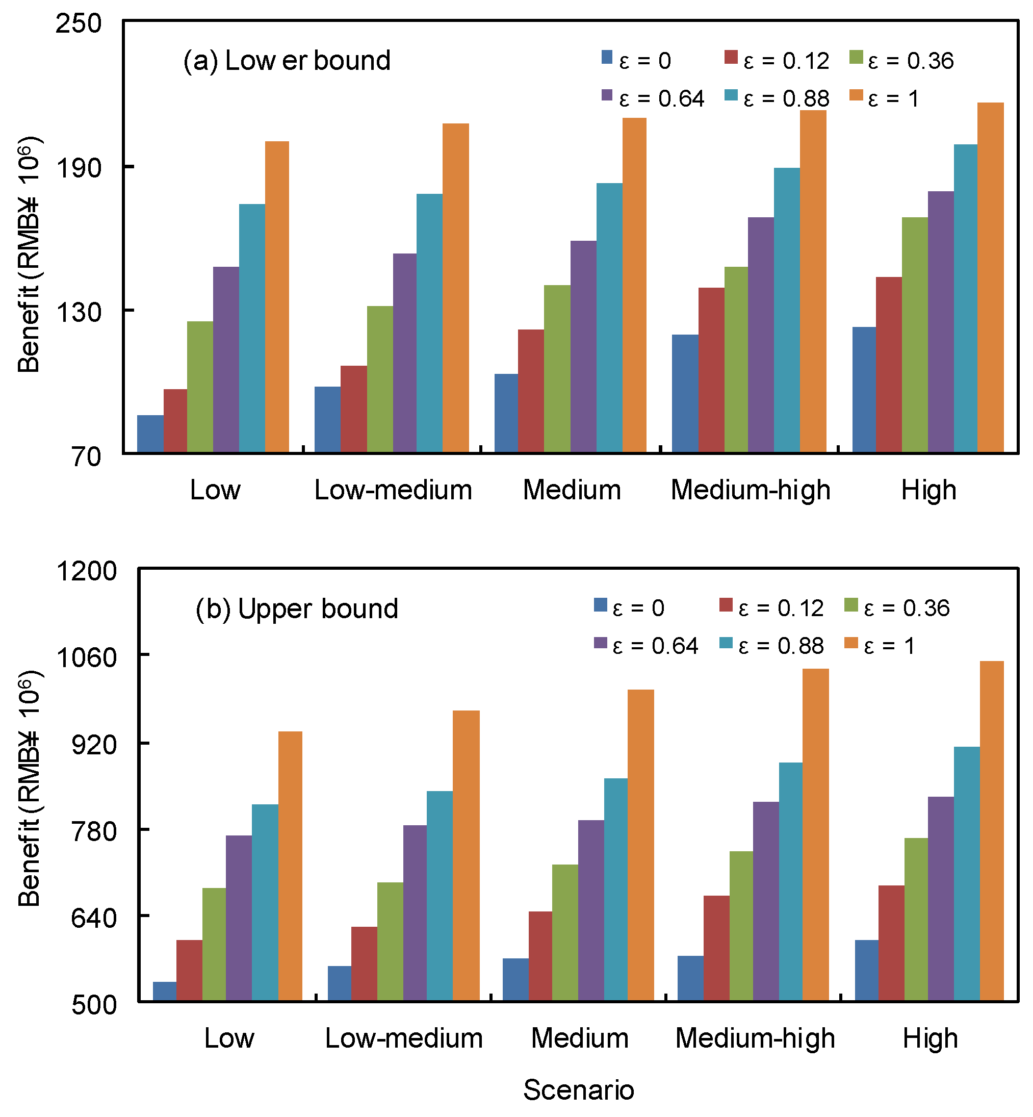
The concept of financial risk was employed to manage the economic loss risk related to the production policy. Figure 4 presents the variation of benefit corresponding to each risk level and pollutant discharge allowance scenario. It is indicated that, under a given scenario, benefit would increase with the ε level. For instance, when pollutant discharge allowance is low, the system benefit would be RMB¥ [124.8, 685.6] × 106 under ε = 0.36 and RMB¥ [173.7, 820.1] × 106 under ε = 0.88, respectively. The higher risk level corresponds to a higher targeted benefit and thus a higher production level, leading to a higher benefit. A straightforward way of evaluating the tradeoff between risk and benefit is to use the cumulative risk curve. Figure 5 illustrates the lower and upper bound cumulative risk curves under different risk levels, respectively. Under a fixed ε level, the cumulative risk curve indicates the level of incurred risk for the generation target at each benefit level (which is the difference between regular benefit and penalty under a designed pollutant discharge allowance scenario). The cumulative risk curves would monotonically increase because they are cumulative probability functions; therefore, the risk is given by the cumulative probability. The risk area would increase as the ε level is raised. Generally, decisions at a lower ε level (i.e., risk averse) would lead to an increased reliability in fulfilling the system requirements but with a lower system benefit; conversely, a strong desire to obtain high system benefit (i.e., risk neutral or risk prone) would yield a raised risk of violating the constraints. It is revealed that a tradeoff between system benefit and system failure risk exists in the decision processes.
4.3. Proportion of Benefit under Different Scenarios
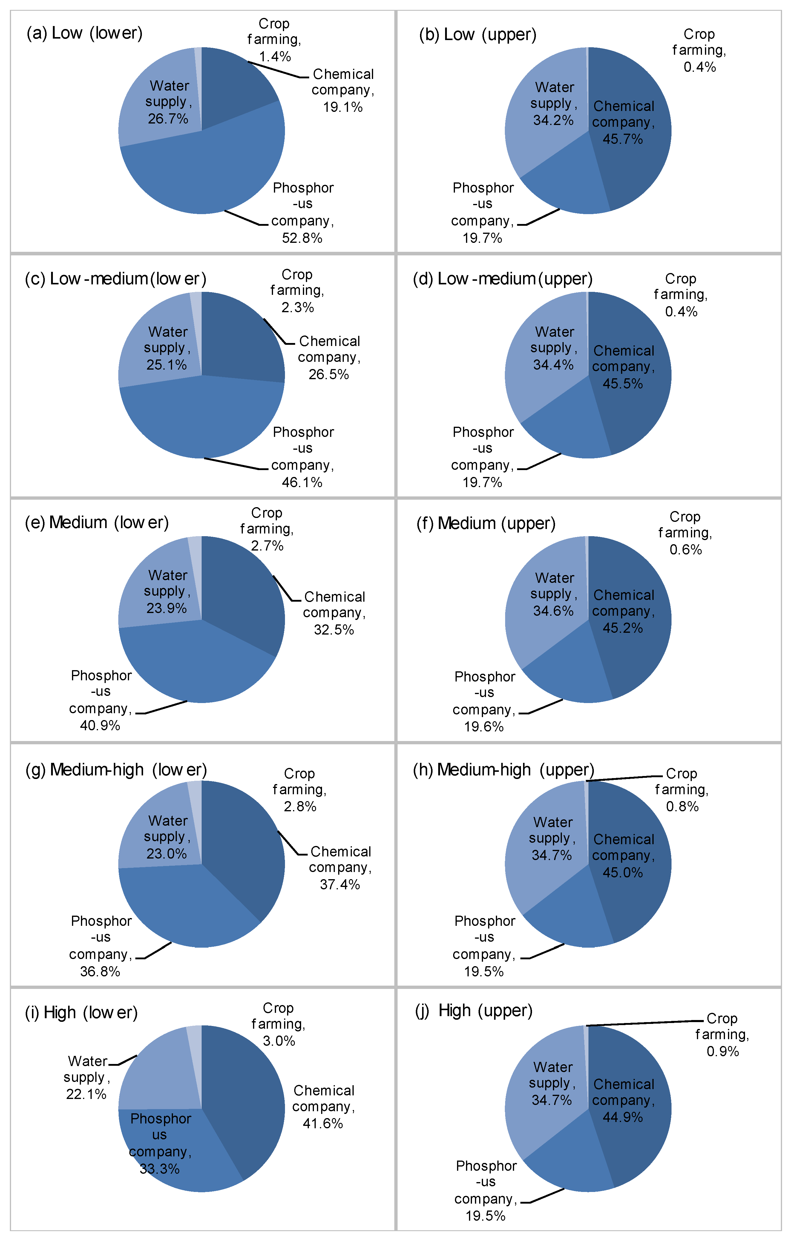
Figure 6 presents proportion of benefit from all activities (including chemical plant, phosphorus mining company, water supply, and crop farming) under different scenarios. As shown in Figure 6, over the planning horizon, benefits from chemical plant and phosphorus mining company would be ranked as the first and the second proportion. For instance, under high scenario, the proportions would be [19.5, 33.3]% and [41.6, 44.9]%, respectively. This is due to the fact that the there are plenty of mineral resources (particularly phosphate ore) in the watershed; meanwhile, unit benefit of mineral related production is high (leading to phosphorus related industry-oriented pattern). In addition, crop farming would produce less than 3% of the benefit due to its low crop yield and limited arable land. Under low scenario, it would only produce [0.4, 1.4]% of the total benefit. However, crop farming is an important income source for rural households, which accounts for about 73% of the total population. Thus, how to enhance crop yield would be a huge concern to the decision makers.
4.4. Optimal Production Target and Actual Production Level
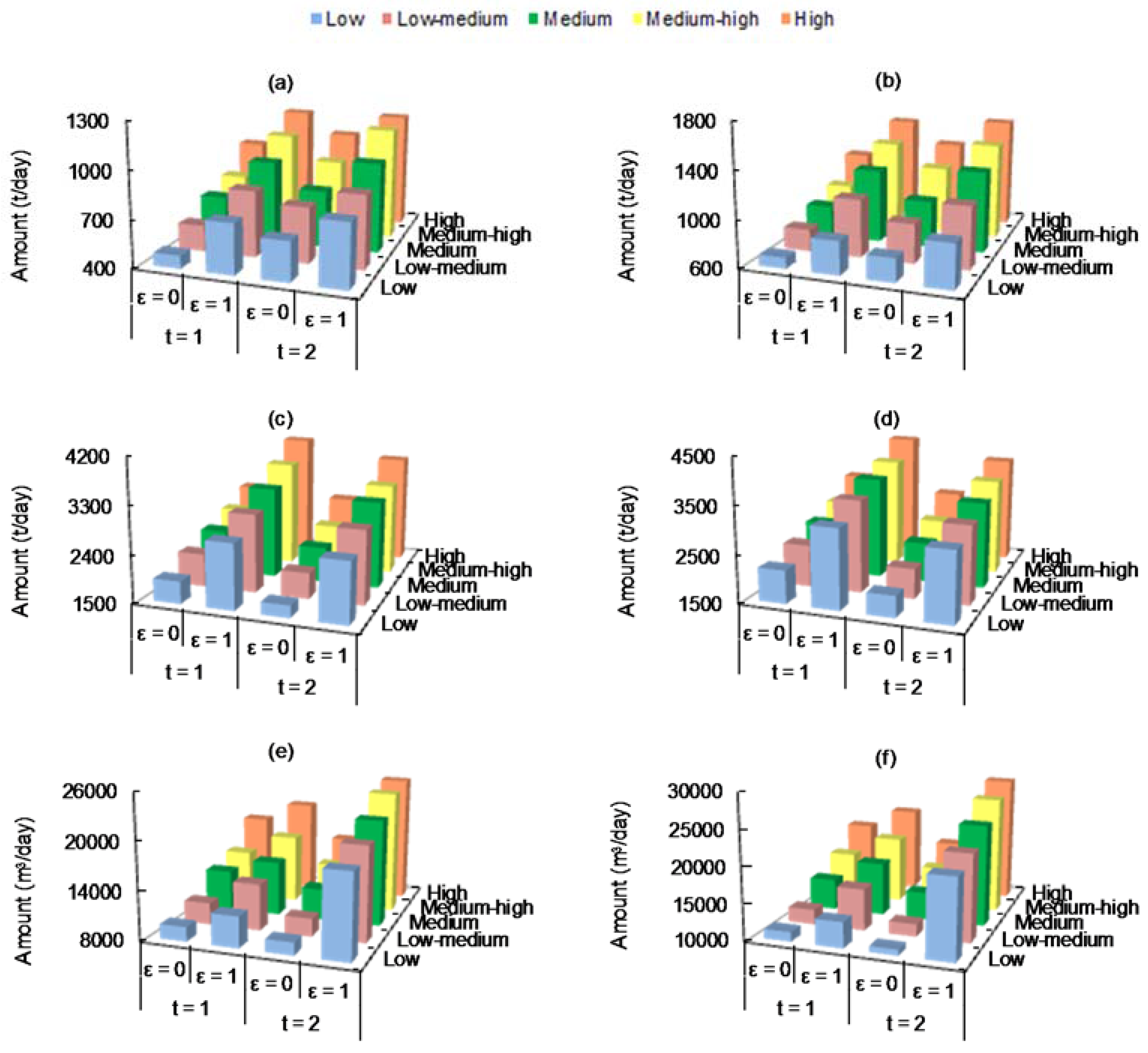
Table 3 provides the optimal production targets under different ε levels. Results obtained reveal that different risk levels lead to changed optimal production targets. For example, in period 1, the total targets of all chemical plants would change from 1279.4 t/day (ε = 0) to 1618.5 t/day (ε = 1). The increment of target is mainly derived from raised targeted benefits along with risk attitudes of decision makers. Figure 7 shows the corresponding results of actual production levels within the optimal production targets. It is indicated that the actual production levels would increase with the raised risk levels and pollutant discharge allowance scenarios. For instance, under low scenario (t = 1), production level of chemical plant would change from [412.4, 733.9] t/day (ε = 0) to [794.5, 883.7] t/day (ε = 1). Under a fixed ε level of 1, production level of chemical plant would be [681.4, 832.7] t/day (with low-medium scenario) and [1278.2, 1743.2] t/day (with high scenario). Results reveal that such changes would be mainly associated with risk attitudes of decision makers and allowable pollutant discharges.
4.5. Excess Pollutant Discharge
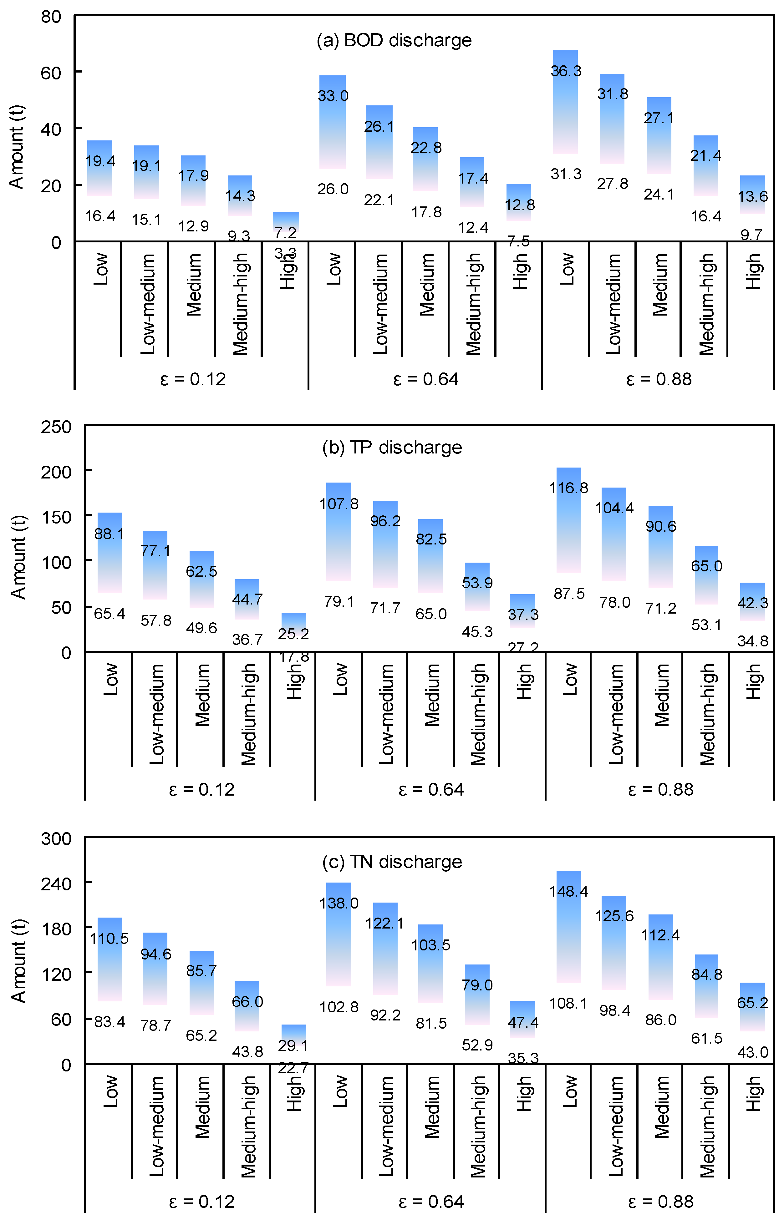
Figure 8 describes the excess BOD, TN, and TP discharges under different ε levels. Different ε levels would result in different production levels, leading to different pollutant loadings. Results indicate that the excess BOD, TN, and TP discharges would increase as ε level is raised. For instance, under medium scenario, the total amounts of excess BOD, TN, and TP discharges would respectively approach [12.9, 18.1] t, [49.6, 62.5] t, and [65.2, 85.7] t (i.e., tonne) under ε = 0.12, while they would be [24.1, 28.9] t, [71.2, 90.6] t, and [86.6, 112.4] t under ε = 0.88, respectively. This is due to the fact that higher ε levels correspond to optimal production targets of economic activities, leading to higher pollutant discharges. Decision makers could justify pollutants control schemes according to the risk levels. Besides, chemical plant would be the main BOD and TP dischargers (associated with its high pollutant discharge rate and production level), while crop farming would be the main TN contributor (due to heavy runoff and soil loss). Thus, advanced wastewater treatment technologies (e.g., tertiary wastewater treatment and depth processing technologies) should be recommended to further improve pollutant removal efficiency. Moreover, some ecologically engineered management measures (e.g., constructed wetland, buffer stripes, and river channel enhancement zone) can be taken to mitigate soil loss and nutrient losses.
5. Conclusions
In this study, a semi-infinite interval-stochastic risk management (SIRM) model has been proposed through integrating the concepts of financial risk management and functional interval parameters into a two-stage stochastic programming (TSP) framework. The SIRM model can handle uncertainties described as probability distributions and functional interval values. Economic penalty is imposed when random variables are violated after the realization of designed targets. Decision makers' attitudes towards system risk are reflected using a risk management measure by controlling the variability of the second-stage cost (i.e., penalty). The SIRM model enables decision makers to account for uncertainty in alternative evaluation and comparison, and help maximize the expected benefit as well as minimize the financial risk at every benefit level. The SIRM model has been applied to water quality management in the Xiangxihe watershed. A number of pollutants (i.e., BOD, TN, TP) generated by industrial and agricultural activities have been considered. Interval solutions with different risk levels and allowable pollutant discharge scenarios concerning optimal production target, actual production level, and excess pollutant discharge have been generated through solving the model.
Results disclose that uncertainties and risks have significant effects on the watershed's production generation pattern and pollutant control schemes as well as the system benefit and economic penalty. It is revealed that the optimal production target and actual production level would increase with a raised risk level (i.e., a risk-neutral attitude to the system failure); under each ε level, more pollutant would be generated due to the increased allowable pollutant discharges. Under a fixed ε level, higher allowable pollutant discharge corresponds to a higher production level, resulting in a higher benefit. Moreover, under a given scenario, benefit would increase with the ε level; higher risk level corresponds to a higher targeted benefit and thus a higher production level, leading to a higher benefit. In summary, decisions at a lower ε level (i.e., risk averse) would lead to an increased reliability in fulfilling the system requirements but with a lower system benefit; conversely, a strong desire to obtain high system benefit (i.e., risk neutral or risk prone) would yield a raised risk of violating the constraints.
On the other hand, results disclose that chemical plant and phosphorus mining company would be the main income source of the study area (occupying more than 60% of the total benefit), while chemical plant would be the main BOD and TP dischargers (account for more than 72% and 75% of the total BOD and TP dischargers, respectively). Although crop farming would produce less than 3% of the total benefit, it would be the main TN contributor due to heavy runoff and soil loss (crop farming discharge 82% of the total TN discharge). Abatement of pollutant contaminations from industrial and agricultural activities is important for the river pollution control. However, the implementation of management practices for water pollution control can have potentials to affect the local economic income. There is a tradeoff between the economic income and pollution control. Several suggestions that could help local authority generate desired decision schemes in association with both maximizing economic income and reducing water pollution are: (i) wastewater treatment technologies (e.g., tertiary treatment and depth processing technologies) would be enhanced to improve the pollutant removal efficiency; (ii) definite land management alternatives suitable to legally manage the farmland need to be enacted for controlling soil erosion; (iii) some ecologically engineered management measures (e.g., constructed wetland, buffer stripes, and river channel enhancement zone) can also be taken to mitigate nitrogen and phosphorus losses.
The first attempt to employ the SIRM model to support water quality management of a watershed system demonstrates its applicability. However, the SIRM model still has space for further improvement. Firstly, it has difficulties in tackling uncertainties expressed as possibility distributions (i.e., fuzzy uncertainties). For example, decision makers’ estimations of pollutant discharge allowances are objectively determined relying on some available historical data; the observed values of them may be ambiguous that can be estimated as fuzzy sets, leading to more complex uncertainties (e.g., intervals with fuzzy-random boundary). The shortcoming can be overcome by incorporating fuzzy mathematical programming into the SIRM framework. Secondly, the effects of the uncertainties as well as their interactions on the water quality management system performance should be further disclosed. Multi-level factorial design can effectively identify the important parameters (or factors) and detect their interactions on modelling outputs. Thirdly, decision support regarding pollution concentration management could be further provided by incorporating certain water quality simulation models into the SIRM framework, which can effectively reflect dynamic interactions between pollutant loading and water quality.
Acknowledgements
This research was supported by the National Key Research Development Program of China (2016YFA0601502 and 2016YFC0502800), and the 111 Project (B14008). The authors are grateful to the editors and the anonymous reviewers for their insightful comments and suggestions.
Author Contributions
Yongping Li and Guohe Huang conceived and designed the experiments; Jing Liu performed the experiments; Jing Liu and Yurui Fan analyzed the data; Jing Liu contributed reagents/materials/analysis tools; Jing Liu wrote the paper.
Conflicts of Interest
The authors declare no conflict of interest.
Appendix A. Solution Method
In SIRM model, the first-stage decision variables in the model are expressed as intervals, which should be identified before the random variables are disclosed. Consequently, decision variables are introduced to identify an optimized set of the first stage values for supporting the related policy analyses. Let , where and . Then, a two-step process is proposed to transform the model into two deterministic submodels that are associated with the lower and upper bounds of the desired objective. Since the objective is to be maximized, the submodel corresponding to (i.e., most desirable objective) can be firstly formulated:
subject to:
where , , , and are decision variables; are decision variables with positive coefficients in the objective function; are decision variables with negative coefficients. Solutions of , , , and can be obtained through solving submodel (A1).The optimized first-stage variables are . Then, the submodel corresponding to the lower-bound objective-function value () is:
subject to:
where , , and are decision variables. Solutions of , , and can be obtained through solving submodel (A2). Through integrating the solutions of the two sets of submodels, the solution for the objective function value can be obtained. The detailed computational processes for solving the SIRM model can be summarized as follows:
Step 1. Formulate the SIRM model.
Step 2. Transform the SIRM model into two submodels, based on an interactive algorithm.
Step 3. Formulate and solve the upper bound submodel corresponding to , obtain and , and calculate .
Step 4. Formulate and solve the submodel base on the solutions obtained through step 3, obtain , and calculate .
Step 5. Construct the corresponding risk curve. If the decision maker is satisfied with the current level of risk then stop, otherwise go to step 6.
Step 6. Let the allowable risk level from the decision makers be and the corresponding aspiration benefit level be .
Step 7. Formulate the SIRM problem with the objective being maximized under chosen and .
Step 8. If the decision maker is satisfied with the solutions, then stop. Otherwise, go to Step 6 for the next level.
Appendix B. Nomenclatures of SIRM Model
| i | chemical plant, 1 = Gufu (GF), 2 = Baishahe (BSH), 3 = Pingyikou (PYK), 4 = Liucaopo (LCP), 5 = Xiangjinlianying (XJLY) |
| j | agricultural zone, and j = 1, 2, 3, 4 |
| k | main crop, 1 = citrus, 2 = tea, 3 = wheat, 4 = potato, 5 = rapeseed, 6 = alpine rice, 7 = second rice, 8 = maize, 9 = vegetables |
| n | phosphorus mining company; 1 = Xinglong (XL), 2 = Xinghe (XH), 3 = Xingchang (XC), 4 = Geping (GP), 5 = Jiangjiawan (JJW), 6 = Shenjiashan (SJS) |
| s | town, 1 = Gufu, 2 = Nanyang, 3 = Gaoyang, 4 = Xiakou |
| t | planning time period, 1 = dry season, 2 = wet season |
| Lt | length of period (day) |
| l | independent variable representing time with the range of [0, 180] |
| h | allowable pollutant discharge scenario; h = 1, 2, 3 |
| probability of occurrence allowable pollutant discharge level h (%); | |
| net benefit from chemical plant i in period t (RMB¥/t); | |
| production level of chemical plant i in period t (t/day); | |
| average benefit for per unit phosphate ore (RMB¥/t); | |
| production level of phosphorus mining company n during period t (t/day); | |
| net benefit from water supply to municipal uses (RMB¥/m3); | |
| quantity of water supply to town s in period t (m3/day); | |
| average benefit for agricultural product (RMB¥/t); | |
| planning area of crop k in agricultural zone j during period t (ha); | |
| economic cost when the production targets from plant i in period t are not met (RMB¥/t); | |
| actual production level of plant i under scenario h in period t (t/day); | |
| economic cost when the production targets from company n in period t are not met (RMB¥/t); | |
| actual production level of company n under scenario h in period t (t/day); | |
| economic cost when the water supply targets for town s in period t are not met (RMB¥/m3); | |
| actual water supply level of town s under scenario h in period t (m3/day); | |
| economic cost when the plant targets of crop farm j in period t are not met (RMB¥/ha); | |
| actual plant area of crop farm j under scenario h in period t (ha); | |
| wastewater generation rate of chemical plant i during period t (m3/t) | |
| wastewater generation rate at town s during period t (m3/m3) | |
| capacity of wastewater treatment capacity (WTPs) (m3/day) | |
| capacity of wastewater treatment capacity (chemical plants) (m3/day) | |
| BOD concentration of raw wastewater from chemical plant i in period t (kg/m3) | |
| BOD treatment efficiency in chemical plant i during period t (%) | |
| allowable BOD discharge for chemical plant i under scenario h in period t (kg/day) | |
| BOD concentration of municipal wastewater at town s during period t (kg/m3) | |
| BOD treatment efficiency of WTPs at town s during period t (%) | |
| allowable BOD discharge for WTPs at town s during period t (kg/day) | |
| nitrogen content of soil in agricultural zone j planted with crop k (%) | |
| average soil loss from agricultural zone j planted with crop k in period t (t/ha) | |
| runoff from agricultural zone j with crop k in period t (mm) | |
| dissolved nitrogen concentration in runoff from agricultural zone j planted with crop k in period t (mg/L) | |
| maximum allowable nitrogen loss in agricultural zone j under scenario h during period t (t) | |
| phosphorus concentration of raw wastewater from chemical plant i in period t (kg/m3) | |
| phosphorus treatment efficiency in chemical plant i in period t (%) | |
| amount of slag discharged by chemical plant i in period t (kg/t) | |
| slag loss rate due to rain wash in chemical plant i during period t (%) | |
| phosphorus content in slag generated by chemical plant i in period t (%) | |
| allowable phosphorus discharge for chemical plant i under scenario h in period t (kg/day) | |
| phosphorus concentration of municipal wastewater at town s in period t (kg/m3) | |
| phosphorus treatment efficiency of WTP at town s in period t (%) | |
| allowable phosphorus discharge for WTP at town s under scenario h in period t (kg/day) | |
| wastewater generation from phosphorus mining company n in period t (m3/t) | |
| phosphorus concentration of wastewater from mining company n in period t (kg/ m3) | |
| phosphorus treatment efficiency in mining company n (%) | |
| amount of slag discharged by mining company n during period t (kg/t) | |
| phosphorus content in generated slag (%) | |
| slag loss rate due to rain wash (%) | |
| allowable phosphorus discharge for mining company n under scenario h during period t (kg/day) | |
| phosphorus content of soil in agricultural zone j planted with crop k (%) | |
| average soil loss from agricultural zone j planted with crop k in period t (t/ha) | |
| dissolved phosphorus concentration in runoff from agricultural zone j with crop k (mg/L) | |
| maximum allowable phosphorus loss in agricultural zone j under scenario h in period t (t/ha) | |
| maximum allowable soil loss agricultural zone j under scenario h in period t (t) | |
| targeted benefit level of economic activities (RMB¥) | |
| integer variable, which would take a value of zero if the benefit for each economic activity under scenario h is greater than or equal to the target level () and a value of one otherwise | |
| upper bound benefit under each scenario h (RMB¥) | |
| desired risk exposure level of economic activity | |
| the government requirement for minimum area of farmland during period t (ha); | |
| minimum production level of chemical plant i in period t (t/day) | |
| maximum production level of chemical plant i in period t (t/day) | |
| minimum quantity of water supply to town s in period t (m3/day) | |
| maximum quantity of water supply to town s in period t (m3/day) | |
| minimum production level of phosphorus mining company n during period t (t/day) | |
| maximum production level of phosphorus mining company n during period t (t/day) |
References
- Ministry of Water Resources, People’s Republic of China. China Water Resources Bulletin; China Water Power Press: Beijing, China, 2017.
- Cederkvist, K.; Jensen, M.B.; Ingvertsen, S.T.; Holm, P.E. Controlling stormwater quality with filter soil—Event and dry weather testing. Water 2016, 8, 349. [Google Scholar] [CrossRef]
- He, J. Probabilistic evaluation of causal relationship between variables for water pollution control. J. Environ. Inform. 2016, 28, 110–119. [Google Scholar] [CrossRef]
- Toyosada, K.; Otani, T.; Shimizu, Y.; Managi, S. Water quality study on the hot and cold water supply systems at Vietnamese Hotels. Water 2017, 9, 251. [Google Scholar] [CrossRef]
- Li, Y.P.; Zhang, N.; Huang, G.H.; Liu, J. Coupling fuzzy-chance constrained program with minimax regret analysis for water pollution control. Stoch. Environ. Res. Risk Assess. 2014, 28, 1769–1784. [Google Scholar] [CrossRef]
- Li, Y.P.; Huang, G.H. Fuzzy-stochastic-based violation analysis method for planning water resources management systems with uncertain information. Inf. Sci. 2009, 179, 4261–4276. [Google Scholar] [CrossRef]
- Li, Y.P.; Huang, G.H. Two-stage planning for sustainable water-quality management under uncertainty. J. Environ. Manag. 2009, 90, 2402–2413. [Google Scholar] [CrossRef] [PubMed]
- Liu, J.; Li, Y.P.; Huang, G.H.; Nie, S. Development of a fuzzy-boundary interval programming method for water pollution control under uncertainty. Water Resour. Manag. 2014, 29, 1169–1191. [Google Scholar] [CrossRef]
- Kerachian, R.; Karamouz, M. A stochastic conflict resolution model for water pollution control in reservoir-river systems. Adv. Water Resour. 2007, 30, 866–882. [Google Scholar] [CrossRef]
- Li, Y.P.; Huang, G.H.; Yang, Z.F.; Nie, S.L. IFMP: Interval-fuzzy multistage programming for water resources management under uncertainty. Resour. Conserv. Recycl. 2008, 52, 800–812. [Google Scholar] [CrossRef]
- Ocampo-Duque, W.; Osorio, C.; Piamba, C.; Schuhmacher, M.; Domingo, J.L. Water quality analysis in rivers with non-parametric probability distributions and fuzzy inference systems: Application to the Cauca River, Colombia. Environ. Int. 2013, 52, 17–18. [Google Scholar] [CrossRef] [PubMed]
- Mohammad, R.N.; Najmeh, M. Water quality zoning using probabilistic support vector machines and self-organizing maps. Water Resour. Manag. 2013, 27, 2577–2594. [Google Scholar] [CrossRef]
- Chen., C.F.; Tsai, L.Y.; Fan, C.H.; Lin, J.Y. Using exceedance probability to determine total maximum daily loads for reservoir water pollution control. Water 2016, 8, 541. [Google Scholar] [CrossRef]
- Hwang, S.A.; Hwang, S.J.; Park, S.R.; Lee, S.W. Examining the relationships between water shed urban land use and stream water quality using linear and generalized additive models. Water 2016, 8, 155. [Google Scholar] [CrossRef]
- Ji., Y.; Huang, G.H.; Sun, W.; Li, Y.F. Water pollution control in a wetland system using an inexact left-hand-side chance-constrained fuzzy multi-objective approach. Stoch. Environ. Res. Risk Assess 2016, 30, 621–633. [Google Scholar] [CrossRef]
- Zolfagharipoor, M.A.; Ahmadi, A. A decision-making framework for river water pollution control under uncertainty: Application of social choice rules. J. Environ. Manag. 2016, 183, 152–163. [Google Scholar] [CrossRef] [PubMed]
- Chen, Y.; Zou, R.; Han, S.; Bai, S.; Faizullabhoy, M.; Wu, Y.Y.; Guo, H.C. Development of an integrated water quality and macroalgae simulation model for Tidal Marsh eutrophication control decision support. Water 2017, 9, 277. [Google Scholar] [CrossRef]
- Li, Y.P.; Huang, G.H.; Huang, Y.F.; Zhou, H.D. A multistage fuzzy-stochastic programming model for supporting sustainable water resources allocation and management. Environ. Model. Softw. 2009, 24, 786–797. [Google Scholar] [CrossRef]
- Nematian, J. An extended two-stage stochastic programming approach for water resources management under uncertainty. J. Environ. Inform. 2016, 27, 72–84. [Google Scholar] [CrossRef]
- Huang, G.H.; Loucks, D.P. An inexact two-stage stochastic programming model for water resources management under uncertainty. Civ. Eng. Environ. Syst. 2000, 17, 95–118. [Google Scholar] [CrossRef]
- Zhang, N.; Li, Y.P.; Huang, W.W.; Liu, J. An inexact two-stage water pollution control model for supporting sustainable development in a rural system. J. Environ. Inform. 2014, 24, 52–64. [Google Scholar] [CrossRef]
- Luo, B.; Li, J.B.; Huang, G.H.; Li, H.L. A simulation-based interval two-stage stochastic model for agricultural non-point source pollution control through land retirement. Sci. Total Environ. 2006, 361, 38–56. [Google Scholar] [CrossRef] [PubMed]
- Harrison, K.W. Two-stage decision-making under uncertainty and stochasticity: Bayesian Programming. Adv. Water Resour. 2007, 30, 641–664. [Google Scholar] [CrossRef]
- Tavakoli, A.; Nikoo, M.R.; Kerachian, R.; Soltani, M. River water pollution control considering agricultural return flows: Application of a nonlinear two-stage stochastic fuzzy programming. Environ. Monit. Assess. 2015, 187, 158. [Google Scholar] [CrossRef] [PubMed]
- Hu, X.H.; Li, Y.P.; Huang, G.H.; Zhuang, X.W.; Ding, X.W. A Bayesian-based two-stage inexact optimization method for supporting stream water pollution control in the three gorges reservoir region. Environ. Sci. Pollut. Res. 2016, 23, 9164–9182. [Google Scholar] [CrossRef] [PubMed]
- Ahmed, S.; Sahinidis, N.V. Robust process planning under uncertainty. Ind. Eng. Chem. Res. 1998, 37, 1883–1892. [Google Scholar] [CrossRef]
- Li, Y.P.; Huang, G.H. Interval-parameter robust optimization for environmental management under uncertainty. Can. J. Civ. Eng. 2009, 36, 592–606. [Google Scholar] [CrossRef]
- Khan, U.T.; Valeo, C. Short-term peak flow rate prediction and flood risk assessment using fuzzy linear regression. J. Environ. Inform. 2016, 28, 71–89. [Google Scholar] [CrossRef]
- Koppol, A.P.R.; Bagajewicz, M.J. Financial risk management in the design of water utilization systems in process plants. Ind. Eng. Chem. Res. 2004, 42, 5249–5255. [Google Scholar] [CrossRef]
- Barbaro, A.; Bagajewicz, M.J. Managing financial risk in planning under uncertainty. Process Syst. Eng. 2004, 50, 963–989. [Google Scholar] [CrossRef]
- Liu, Z.F.; Huang, G.H. Dual-interval two-stage optimization for flood management and risk analyses. Water Resour. Manag. 2009, 23, 2141–2162. [Google Scholar] [CrossRef]
- Ahmed, S.; Elsholkami, M.; Elkamel, A.; Du, J.; Ydstie, E.B.; Douglas, P.L. Financial risk management for new technology integration in energy planning under uncertainty. Appl. Energy 2014, 128, 75–81. [Google Scholar] [CrossRef]
- Zhu, Y.; Li, Y.P.; Huang, G.H. Planning carbon emission trading for Beijing’s electric power systems under dual uncertainties. Renew. Sustain. Energy Rev. 2013, 23, 113–128. [Google Scholar] [CrossRef]
- Felfel, H.; Ayadi, O.; Masmoudi, F. Multi-objective stochastic multi-site supply chain planning under demand uncertainty considering downside risk. Comput. Ind. Eng. 2016, 102, 268–279. [Google Scholar] [CrossRef]
- McCray, A.W. Petroleum Evaluations and Economic Decisions; Prentice Hall: Englewood Cliffs, NJ, USA, 1975; ISBN 0136622136. [Google Scholar]
- Chen, H.W.; Chang, N.B. Decision support for allocation of watershed pollution load using grey fuzzy multobjective programming. J. Am. Water Resour. Assoc. 2006, 42, 725–745. [Google Scholar] [CrossRef]
Figure 1.
Overall flow chat of the methodology.
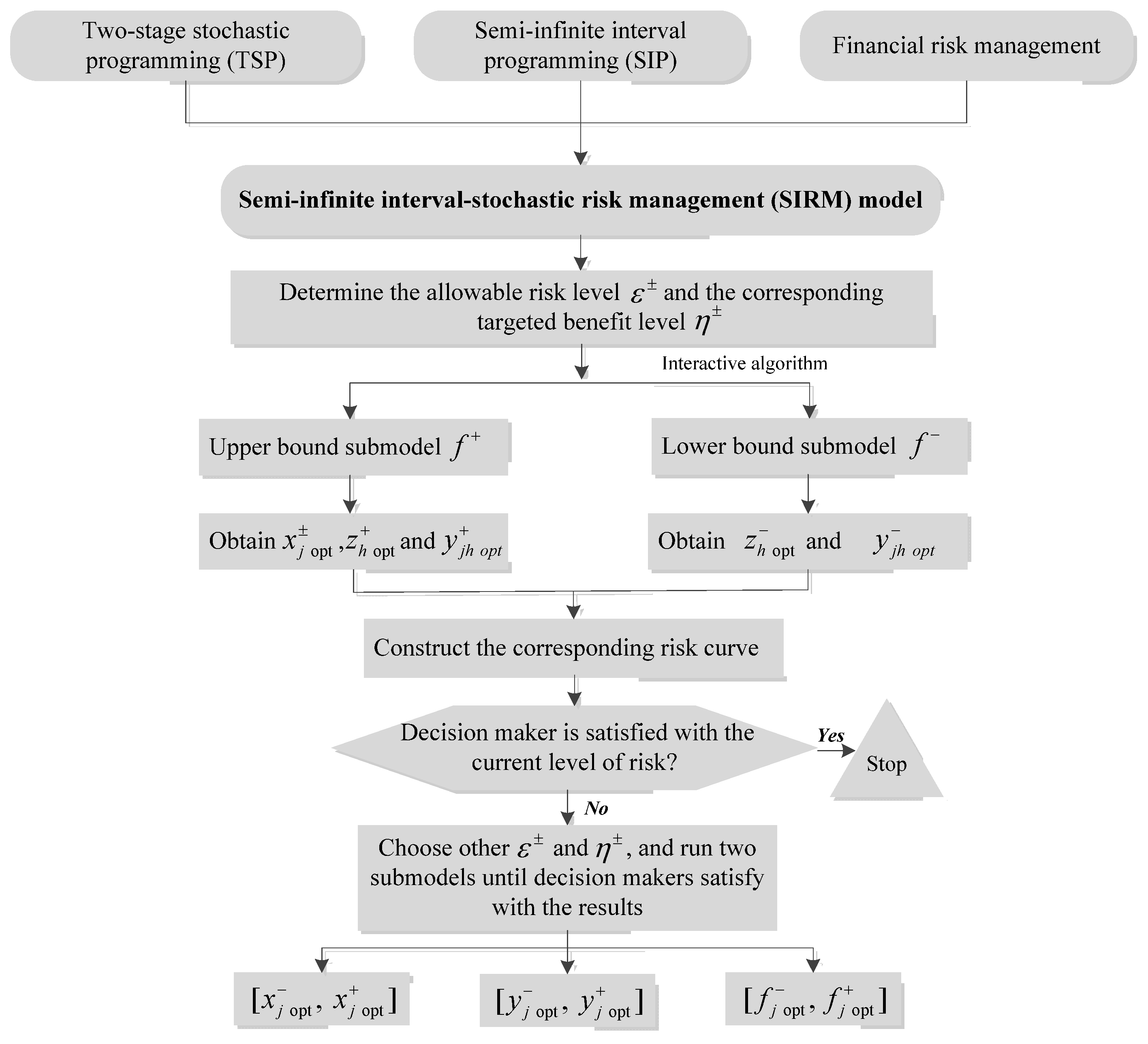
Figure 2.
Study area. Note: GF, Gufu chemical plant; XL, Xinglong phosphorus mining company; XH, Xinghe phosphorus mining company; XC, Xingchang phosphorus mining company; BSH, Baishahe chemical plant; PYK, Pingyikou chemical plant; LCP, Liucaopo chemical plant; GP, Geping phosphorus mining company; JJW, Jiangjiawan phosphorus mining company; SJS, Shenjiashan phosphorus mining company; XJLY, Xiangjinlianying chemical plant.

Figure 3.
Benefits and costs under different risk levels. Note: (a) lower-bound targeted benefit and system benefit, (b) upper-bound targeted benefit and system benefit, (c) lower-bound regular benefit and penalty, (d) upper-bound regular benefit and penalty; unit: 106 RMB¥.
Figure 3.
Benefits and costs under different risk levels. Note: (a) lower-bound targeted benefit and system benefit, (b) upper-bound targeted benefit and system benefit, (c) lower-bound regular benefit and penalty, (d) upper-bound regular benefit and penalty; unit: 106 RMB¥.
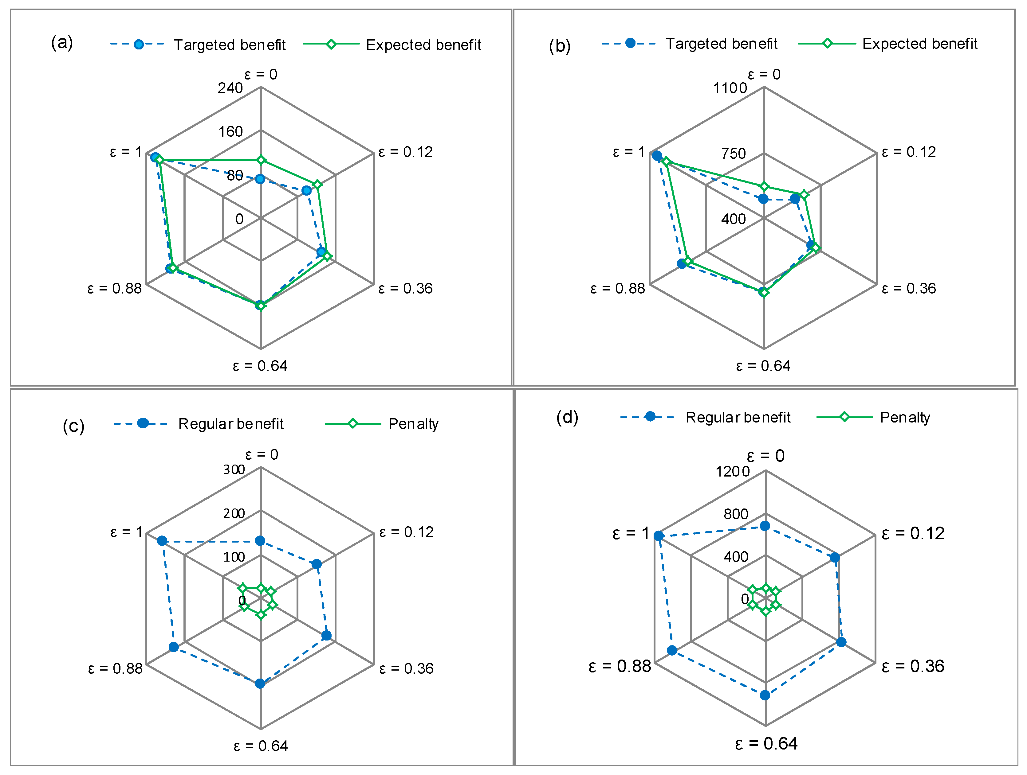
Figure 4.
Benefit corresponding to each scenario and risk level. (a) Lower bound and (b) Upper bound.
Figure 4.
Benefit corresponding to each scenario and risk level. (a) Lower bound and (b) Upper bound.

Figure 5.
Cumulative risk curve ((a) Lower bound and (b) Upper bound).
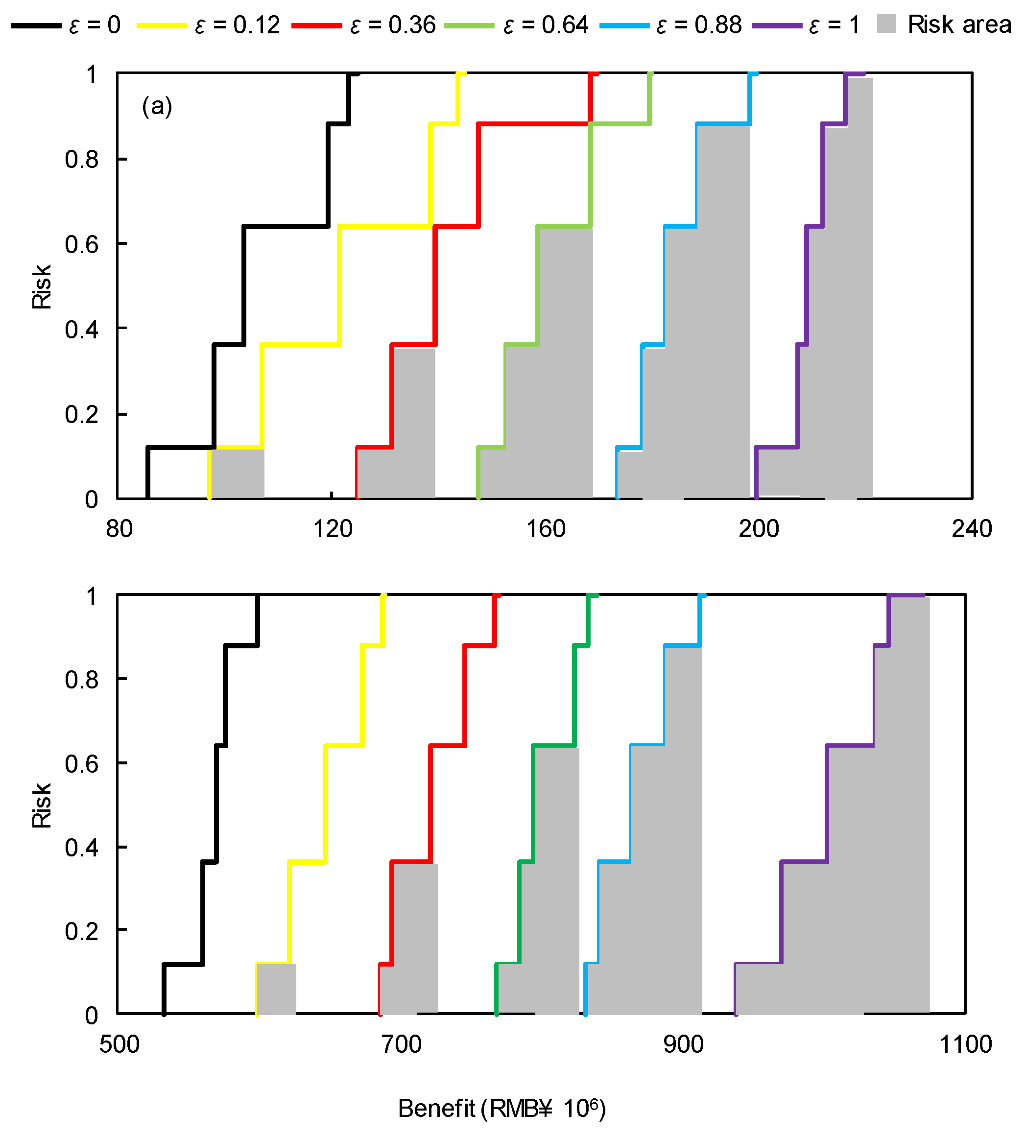
Figure 6.
Proportion of benefit under different scenarios. (a) Lower bound under low scenario; (b) Upper bound under low scenario; (c) Lower bound under low-medium scenario; (d) Upper bound under low-medium scenario; (e) Lower bound under medium scenario; (f) Upper bound under medium scenario; (g) Lower bound under medium-high scenario; (h) Upper bound under medium-high scenario; (i) Lower bound under high scenario and (j) Upper bound under high scenario.

Figure 7.
Actual production levels of industrial activities. Note: (a) lower-bound production level of chemical plant; (b) upper-bound production level of chemical plant; (c) lower-bound production level of phosphorus mining company; (d) upper-bound production level of phosphorus mining company; (e) lower-bound water supply and (f) upper-bound water supply.

Figure 8.
Excess Pollutant Discharge. (a) BOD discharge; (b) TP discharge and (c) TN discharge.

Table 1.
Net benefits and penalties from industrial activities.
| Industrial Activities | Net Benefit | Penalty | ||
|---|---|---|---|---|
| Period 1 | Period 2 | |||
| Chemical plant (RMB¥/t) | ||||
| Gufu (GF) | [791.3, 832.4] | [803.2, 864.7] | [823.6, 891.5] | [833.1, 910.4] |
| Baishahe (BSH) | [1217.4, 1493.8] | [1532.3, 1682.4] | [1357.4, 1634.1] | [1723.7, 1841.6] |
| Pingyikou (PYK) | [832.8, 912.4] | [943.5, 1032.4] | [861.5, 943.8] | [993.5, 1145.7] |
| Liucaopo (LCP) | [1532.6, 1843.5] | [1682.2, 1942.5] | [1735.7, 2011.1] | [1835.3, 2113.5] |
| Xiangjinlianying (XJLY) | [1843.3, 2174.3] | [1932.4, 2243.5] | [1992.3, 2294.5] | [2014.5, 2385.3] |
| Water supply (RMB¥/m3) | ||||
| Gufu | [45.4, 52.7] | [58.8, 61.4] | [52.4, 58.9] | [63.7, 68.2] |
| Nanyang | [32.4, 38.5] | [41.4, 46.7] | [39.5, 43.1] | [47.2, 53.4] |
| Gaoyang | [48.3, 52.4] | [56.4, 59.4] | [55.5, 58.7] | [63.7, 70.1] |
| Xiakou | [42.1, 46.2] | [48.3, 53.4] | [49.2, 54.5] | [53.8, 59.1] |
| Phosphorus mining company (RMB¥/t) | ||||
| Xinglong (XL) | [167.3, 185.3] | [167.3, 194.2] | [196.7, 213.5] | [196.7, 221.3] |
| Xinghe (XH) | [154.5, 164.9] | [163.4, 173.4] | [178.4, 197.3] | [182.1, 207.3] |
| Xingchang (XC) | [161.5, 178.4] | [161.5, 178.4] | [188.4, 204.5] | [188.4, 204.5] |
| Geping (GP) | [166.4, 174.7] | [168.3, 179.4] | [189.2, 201.3] | [191.2, 207.3] |
| Jiangjiawan (JJW) | [161.4, 178.6] | [166.4, 181.4] | [188.3, 204.6] | [189.2, 211.3] |
| Shenjiashan (SJS) | [161.4, 183.4] | [171.9, 191.5] | [188.3, 211.3] | [198.2, 201.4] |
Table 2.
Allowable pollutant discharges for industrial activities.
| Industrial Activities | Period 1 | Period 2 |
|---|---|---|
| Allowable phosphorus discharge for each chemical plant (kg/day) | ||
| Gufu (GF) | [0.60 + 0.002l, 1.05 + 0.002l] | [0.70 + 0.001l, 1.15 + 0.001l] |
| Baishahe (BSH) | [195.63 + 0.089l, 432.56 + 0.089l] | [162.64 + 0.086l, 407.87+ 0.086l] |
| Pingyikou (PYK) | [30.49 + 0.09l, 70.71+ 0.09l] | [50.03 + 0.013l, 90.30 + 0.013l] |
| Liucaopo (LCP) | [124.7 + 0.046l, 294.7 + 0.046l] | [213.40 + 0.043l, 409.5 + 0.043l] |
| Xiangjinlianying (XJLY) | [126.22 + 0.042l, 321.76 + 0.042l] | [174.4 + 0.039l, 364.8 + 0.039l] |
| Allowable phosphorus discharge for each mine company (kg/m3) | ||
| Xinglong (XL) | [47.41 + 0.043l, 123.49 + 0.043l] | [78.31 + 0.41l, 191.59 + 0.041l] |
| Xinghe (XH) | [23.68 + 0.044l, 86.87 + 0.044l] | [39.19 + 0.42l, 86.87 + 0.042l] |
| Xingchang (XC) | [30.54 + 0.038l], 62.75, + 0.038l] | [52.74 + 0.034l, 115.76 + 0.034l] |
| Geping (GP) | [48.39 + 0.012l, 109.36 + 0.012l] | [70.03 + 0.011l, 173.95 + 0.011l] |
| Jiangjiawan (JJW) | [25.91 + 0.014l, 40.13 + 0.014l] | [38.49 + 0.013l, [87.51 + 0.013l] |
| Shenjiashan (SJS) | [20.23 + 0.011l, 42.3l + 0.011l] | [28.19 + 0.009l, [82.6l + 0.009l] |
| Allowable BOD discharge for each WTP (kg/day) | ||
| Gufu | [70 + 0.003l, 110 + 0.003l] | [75 + 0.002l, 115 + 0.002l] |
| Nanyang | [3 + 0.0001l, 8 + 0.0001l] | [4 + 0.0009l, 9 + 0.0009l] |
| Gaoyang | [10 + 0.0003l, 25 + 0.0003l] | [12 + 0.0002l, 27 + 0.0002l] |
| Xiakou | [15 + 0.0002l, 28 + 0.0002l] | [17 + 0.0001l, 30 + 0.0001l] |
Table 3.
Optimal production targets under different ε levels.
| Activity | Designed Target | ε = 0 | ε = 1 | |||
|---|---|---|---|---|---|---|
| t = 1 | t = 2 | t = 1 | t = 2 | t = 1 | t = 2 | |
| Production level of chemical plants (t/day) | ||||||
| i = 1 | [21.8, 28.6] | [17.6, 28.3] | 28.6 | 28.3 | 28.6 | 28.3 |
| i = 2 | [457.5, 573.7] | [461.6, 625.6] | 573.7 | 461.6 | 573.7 | 625.6 |
| i = 3 | [69.5, 112.6] | [62.8, 110.5] | 69.5 | 110.5 | 112.6 | 110.5 |
| i = 4 | [347.2, 526.8] | [327.6, 552.4] | 347.2 | 552.4 | 526.8 | 552.4 |
| i = 5 | [260.4, 376.8] | [256.7, 373.7] | 260.4 | 256.7 | 376.8 | 373.7 |
| Production level of phosphorus mining companies (t/day) | ||||||
| n = 1 | [679.4, 1435.6] | [736.5, 1324.5] | 679.4 | 736.5 | 1435.6 | 1324.5 |
| n = 2 | [246.7, 424.5] | [194.6, 412.5] | 424.5 | 412.5 | 424.5 | 412.5 |
| n = 3 | [257.4, 436.4] | [227.5, 415.3] | 436.4 | 415.3 | 436.4 | 415.3 |
| n = 4 | [385.3, 783.5] | [325.6, 704.5] | 783.5 | 704.5 | 783.5 | 704.5 |
| n = 5 | [348.6, 568.4] | [287.4, 503.5] | 568.4 | 503.5 | 568.4 | 503.5 |
| n = 6 | [495.6, 689.4] | [437.8,612.7] | 689.4 | 437.8 | 689.4 | 612.7 |
| Quantity of water supply to towns (m3/day) | ||||||
| s = 1 | [9921.5, 17533.5] | [10385.7, 21756.4] | 9921.5 | 10385.7 | 17533.5 | 21756.4 |
| s = 2 | [729.5, 1232.7] | [798.5, 1463.6] | 1232.7 | 1463.6 | 1232.7 | 1463.6 |
| s = 3 | [2804.5, 3424.5] | [2964.5, 3853.7] | 3424.5 | 3853.7 | 3424.5 | 3853.7 |
| s = 4 | [1428.7, 2104.7] | [1564.6, 2746.4] | 2104.7 | 2746.4 | 2104.7 | 2746.4 |
© 2017 by the authors. Licensee MDPI, Basel, Switzerland. This article is an open access article distributed under the terms and conditions of the Creative Commons Attribution (CC BY) license (http://creativecommons.org/licenses/by/4.0/).
Share and Cite
MDPI and ACS Style
Liu, J.; Li, Y.; Huang, G.; Fan, Y. A Semi-Infinite Interval-Stochastic Risk Management Model for River Water Pollution Control under Uncertainty. Water 2017, 9, 351. https://doi.org/10.3390/w9050351
AMA Style
Liu J, Li Y, Huang G, Fan Y. A Semi-Infinite Interval-Stochastic Risk Management Model for River Water Pollution Control under Uncertainty. Water. 2017; 9(5):351. https://doi.org/10.3390/w9050351
Chicago/Turabian StyleLiu, Jing, Yongping Li, Guohe Huang, and Yurui Fan. 2017. "A Semi-Infinite Interval-Stochastic Risk Management Model for River Water Pollution Control under Uncertainty" Water 9, no. 5: 351. https://doi.org/10.3390/w9050351
Note that from the first issue of 2016, this journal uses article numbers instead of page numbers. See further details here.