Article

Modeling the Multi-Seasonal Link between the Hydrodynamics of a Reservoir and Its Hydropower Plant Operation

1
Department of Civil Engineering, University of Chile, Blanco Encalada 2002, Santiago 8370449, Chile
2
Energy Center, Department of Electrical Engineering, University of Chile, Tupper 2007, Santiago 8370451, Chile
3
Department of Stochastic Simulation and Safety Research for Hydrosystems (IWS/SC SimTech), University of Stuttgart, Pfaffenwaldring 5A, 70569 Stuttgart, Germany
*
Author to whom correspondence should be addressed.
Water 2017, 9(6), 367; https://doi.org/10.3390/w9060367
Submission received: 9 January 2017 / Revised: 10 May 2017 / Accepted: 18 May 2017 / Published: 24 May 2017

Abstract

:
The hydrodynamics of many hydropower reservoirs are controlled by the operation of their power plant, but the associated water quality impact is often poorly understood. In particular, significant hydropeaking operations by hydropower plants affect not only the downstream ecosystem but also the reservoir water temperature. This paper contributes to understanding that link. For this, we coupled a hydrodynamic model (Estuary, Lake and Coastal Ocean Model, ELCOM) to a grid-wide power system scheduling model. In a case study (Rapel, Chile), we observe the behavior of variables related to the flow regime and water quality (including sub-daily hydrologic alteration, seasonal and sub-daily thermal pollution of the downstream river, and vertical mixing in the reservoir). Additionally, we evaluate how environmental constraints (ECs) can improve the conditions for a wet, normal and dry water-type year. We found that the unconstrained operation produces a strong sub-daily hydrologic alteration as well as an intense thermal pollution of the outflow. We show that these effects can clearly be avoided when implementing ECs. The current (unconstrained) vertical mixing makes the reservoir susceptible to algae blooms. Implementing ECs may intensify the stratification in the reservoir near the dam in some scenarios. The grid-wide economic cost of Rapel’s ECs is a modest 0.3%.

1. Introduction

A dam built for hydropower purposes can be understood as an interface that splits a system into a downstream river and an upstream reservoir, such that the reservoir conditions (water quality, quantity, and temperature) provide the boundary condition for the downstream river. Furthermore, the operation rule of the hydropower plant modifies the conditions on both sides of the interface, in particular, the reservoir storage and the magnitude and timing of the outflows [1,2,3,4]. Considering this continuum perspective, the aim of this article is to study and to quantify how operation rules affect the hydrodynamics and water temperature of a hydropower reservoir, and the hydrological and thermal alterations of the downstream river in the context of the power system operations that define when and how much energy the hydropower plant will produce.
Hydropower operation is highly variable over different timescales. On the seasonal and annual time scales, the availability of the water resource usually defines when and how much energy the hydropower plant will generate. Furthermore, in response to short-term fluctuations in power demand, the power plant can show intensive hydropeaking at sub-hourly, hourly and daily levels. This operation can be exacerbated when massive shares of renewable energies are part of the system, as their primary energy profile is not necessarily in phase with energy demand [5,6], and by new power market structures [7]. Altogether, these fluctuations generate an outflow pattern far from the river’s natural flow regime [8], hence severely altering the integrity of freshwater ecosystems [9,10].
The influence of reservoir operation on downstream rivers has widely been studied and described in terms of changes in the flow regime. Poff and Zimmerman [9] analyzed the relationship between flow alteration and ecological responses from over 150 papers of the last four decades and found that adverse effects were reported in over 90% of the cases. Flow alteration affects all the key constituents of the ecosystem, including the health, diversity, and abundance of macroinvertebrates, fish, and riparian vegetation [9,10,11]. To mitigate the adverse effects of extreme flow fluctuations, environmental constraints are an increasingly frequent mitigation measure within the environmental assessment processes of hydropower plants. These may include minimum environmental flows (MIF) or maximum hourly rates of change in the discharges (maximum ramping rates, MRR) [12,13]; as well as minimum levels of stored water.
River regulation affects another essential variable for the ecosystem conservation: water temperature, which, in turn, controls many ecological processes, including the productivity and cycling of nutrients, metabolic rates and growth rates of aquatic organisms [14,15]. Modifying the natural thermal regime of a river is known as thermal pollution [14] and also has numerous and widely recognized ecological consequences [14,15,16]. Thermal pollution has been studied in association with cooling water discharges from thermal power plants (e.g., coal or nuclear) [17]. Hydropower plants with large reservoirs affected by thermal stratification may withdraw water from below its thermocline, releasing cold flows during summer (also termed as cold water pollution). Due to the thermal inertia and depth of reservoirs, the water release during the operation of the hydropower plant is generally different from its natural thermal regime. Similar to the natural flow regime, the natural temperature regime is highly variable and complex. However, in contrast to flow restoration, the discussion of mitigating thermal pollution in regulated rivers is still incipient. Olden [14] points out that a major challenge in restoring natural thermal regimes is demonstrating the availability and success of strategies for temperature management.
Hydropower reservoir operation controls further parameters that impact water temperature, for example, vertical mixing and water elevation. Vertical mixing is the rate at which constituents found in deep waters (nutrients, metals and oxygen demand) is transported to the epilimnion where phytoplankton, fish, and human activity develop. This process is primarily modulated by regional climate (e.g., air temperature, solar radiation, wind speed) [18], and also by inflow plunging and density currents [18], the outlet elevation that defines the location of the density interface [19,20], and the operation rules of the hydropower plant that determine the time and intensity of current induced by outflows [21]. The operation rules of the hydropower plant can also alter the temporal distribution of water elevation in the reservoir (stored volume), which in turn controls the dynamics of phytoplankton throughout changes in water turbidity induced by the inflow of suspended solid concentrations [22]. Although the authors of [21,22] provide significant advances in understanding the link between hydropower operation and hydrodynamics, these studies were conducted in a relatively short time horizon (during summer stratification). The link of hydropower operation rules to the hydrodynamics of the reservoir, which integrates processes between the hydropeaking and the seasonal time-scales (particularly in the long term, i.e., a few years), is still not well understood.
The aim of this article is to study and to quantify how operation rules affect the hydrodynamics and water temperature of a hydropower reservoir and the hydrological and thermal alterations of the downstream river. We will look at a time period of 30 months, with different hydrologic scenarios (wet, normal and dry conditions), and two different operation rules of the hydropower plant (with and without environmental constraints). We will focus on three variables: (1) the outflows of the hydropower plant in the context of sub-daily hydrologic alteration; (2) the outflow temperature related to the thermal alteration in the downstream river; and (3) the vertical mixing across the reservoir that defines the transport rate of deep water constituents to the epilimnion. The main contributions of the present study are understanding: (1) the link between the hydrodynamics of the reservoir and the operational scheduling of the hydropower plant as part of an interconnected power system; (2) the influence of operation rules on outflow water temperature, vertical mixing, and downstream hydrologic alteration; and (3) the impact of hydrologic inflow scenarios on these variables.
The remainder of this article is structured as follows. Section 2 describes the study site: the Rapel reservoir. Furthermore, Section 3 details the methods and Section 4 shows the results of the case study. Finally, Section 5 draws the conclusions.

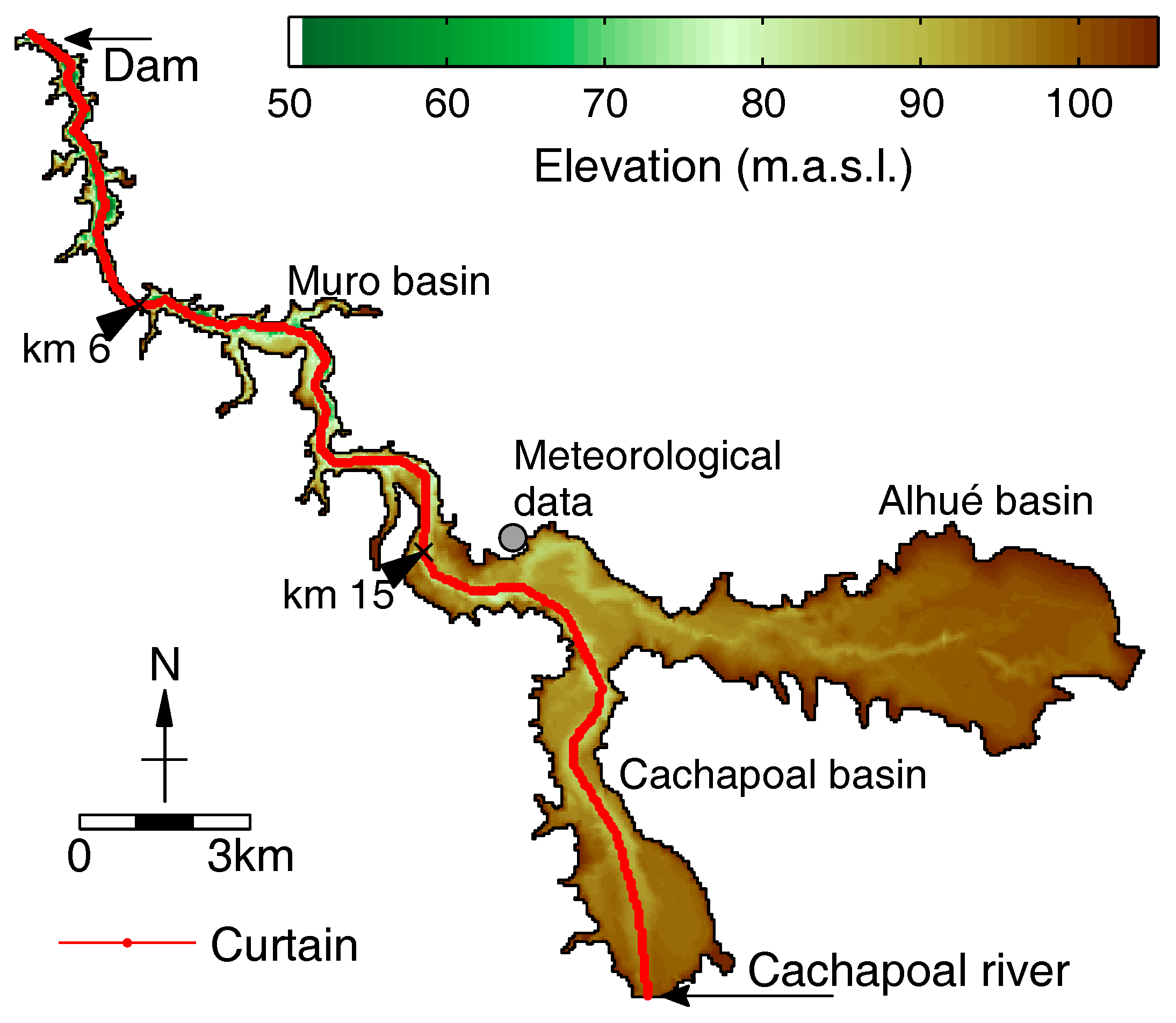
2. Study Site: The Rapel Reservoir

The analysis focuses on the Rapel hydropower reservoir, located in Central Chile (34°2′23″ S, 71°35′23″ W, 110 m above sea level (m.a.s.l.) [23]). The Rapel reservoir has a dendritic shape composed of three basins called Cachapoal, Alhué, and Muro (Figure 1). The main tributaries are the Tinguiririca and Cachapoal rivers, both entering at the upstream end of Cachapoal basin, thus inducing the dominant flow along the Cachapoal-Muro longitudinal curtain (Figure 1) [20,21].
Since its commissioning in 1968, the reservoir has been affected by several events of massive fish death and algae blooms [23]. At the same time, it has become an important place for tourism, which motivated the recent implementation of a minimum reservoir level constraint, required for the normal development of recreational activities like boating.
Rapel is a relatively small reservoir (maximum water depth of 55 m, volume of 400 Hm3, retention time of about two weeks) with a seasonal regulation capacity. As a consequence of the operation scheme, the weekly average outflows are of the same order of magnitude as the weekly average inflows. In the absence of environmental restrictions, its 380 MW power plant produces frequent, significant ramps. Hence, its hourly outflows are coined by a strong peaking operation with very low outflows during most hours, and discharges over 550 m3/s concentrated in a few peak hours of the day. This is exacerbated during the dry season which coincides with the stratification period. Water withdrawal for energy production occurs at the dam between 73 and 88 m above sea level (m.a.s.l.). Further information about the power plant and basin can be found in [20,22,24].

3. Methods

In the present work, we couple a hydrodynamic simulation with a power system scheduling model to study how different hydrologic scenarios and environmental constraints (ECs) of the power plant affect water temperature and hydrologic alteration. We follow a similar methodology (Figure 2) to Rossel and de la Fuente [22]. This coupling is required because the Rapel hydropower plant is part of Chile’s Central Interconnected Power System (SIC), organized as a mandatory pool with audited costs. Thus, the operation of all power plants in central Chile is prescribed by an independent system operator (ISO) following a cost-minimization criterion of the entire power system [5,12]. The following subsections detail this coupling.

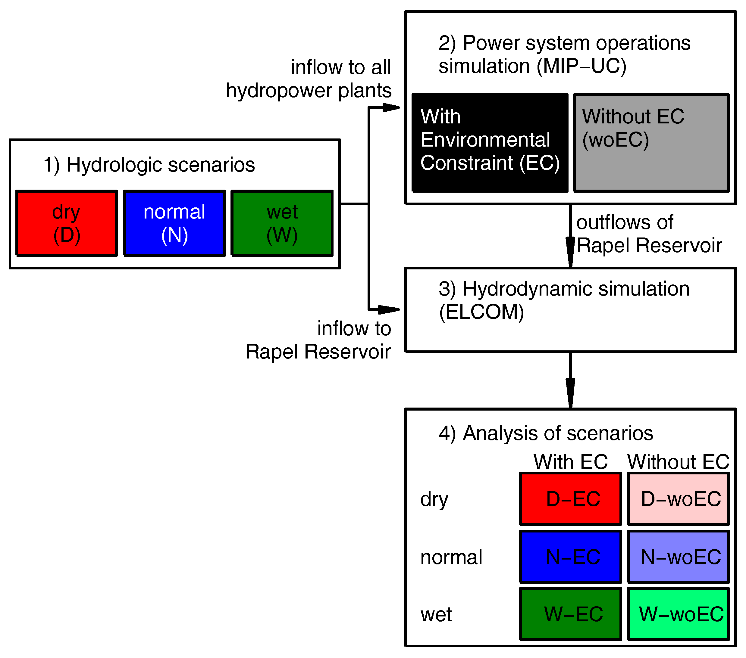
3.1. Hydrologic Scenarios

Three different hydrologic scenarios, wet (W), normal (N) and dry (D), were defined. These correspond to historical years 1986–1987, 1969–1970, and 2007–2008, with a probability of exceedance of their annual flows of 20%, 50%, and 90%, respectively [25]. The record of past flows can be found in the databases of Chile’s ISO [26] and possess a weekly resolution for most hydropower plants. The choice of these values aims at covering a broad spectrum of plausible flows, data availability, and computing capacity limits.
These three scenarios feed into both the power system operations and hydrodynamics model that were continuously run for 30 months. In the power system operations model, these scenarios comprise the inflows to each hydropower plant of the system (including the Rapel reservoir), whereas in the hydrodynamic model they only feed the inflow time series coming into Rapel reservoir. The outflows of Rapel result exclusively from the operation of its power plant, determined by the power system operations model, as explained as follows.

3.2. Power System Operations

To simulate the operation of Rapel we use a tool that replicates the procedure of Chile’s ISO, which relies on a mixed integer optimization to prescribe the unit commitment (MIP-UC) of the whole power grid. The relevant results of the power operation simulation are Rapel’s outflow time series. The model uses an hourly resolution and solves for a weekly horizon. MIP-UC minimizes the operational costs of the power system (composed of thermal, hydro and renewable power plants) while satisfying the energy demand of each node and a set of technical constraints. A detailed formulation of the MIP-UC model can be found in previous studies [12].
The operational costs are mainly associated with thermal plants (coal, gas or diesel). As the system possesses large water reservoirs (besides Rapel), MIP-UC uses an opportunity cost function of stored water (in terms of the stored water at the end of the simulation horizon) [12]. This future cost function is computed by the ISO using a stochastic medium-term optimization tool [27] and can be understood as the displaced future thermal costs.
The technical constraints include water balance, water-to-power-yield and flow routing, minimum and maximum power capacities, minimum on- and off-line times of generators and transmission capacities of the grid (modeled as direct current power flow), including power losses.
The remaining information required for MIP-UP, like fuel cost or the energy demands, are publicly available inputs for the ISO weekly scheduling [28]. The actual conditions from January 2011 to June 2013 were taken.
To mitigate hydrologic alteration, implementing environmental flow constraints are a common solution. In this article, we study the influence of two different sets of scenarios on the hydrodynamics of the reservoir and thermal pollution of the downstream river: with environmental constraint (named EC) and without environmental constraint (named woEC). The EC scenario is a combination of a minimum instream flow (MIF) and a maximum ramping rate of the turbine outflow (MRR). Based on the findings of [12] (which studied the trade-off between the cost of implementing environmental constraints and their effectiveness in improving sub-daily hydrologic alteration), we chose efficient values for our environmental constraints. This resulted in 20% and 6% of the median monthly inflow as MIF and MRR, respectively. In other words, the MIF requires Rapel to release (either through the turbines or the spillway) at all times at least 20% of the median inflows of a given month, and the MRR to operate so smoothly that the changes in turbine outflows between two consecutive hours are always below 6% of the monthly median inflow. The combination of the hydrologic scenarios and the two operational cases (with or without environmental constraints) define six scenarios for the power system operations simulation and the hydrodynamics simulation (Table 1).

3.3. Hydrodynamic Simulation

The hydrodynamics simulation was conducted with the model Estuary, Lake and Coastal Ocean Model (ELCOM) [29,30]. This 3D-hydrodynamics model considers environmental variables (wind speed, irradiation, water in- and outflows, temperature, precipitation, and so forth) to determine the spatial and temporal behavior of water bodies. For the simulation, the same mesh grid as in [21,22] was used, which is based on elements of 50 × 50 m of horizontal spacing, and 2 m of vertical spacing. The meteorological information was obtained from the atmospheric reanalysis ERA-Interim Daily of the European Centre for Medium-Range Weather Forecasts, for the grid point located in the center of the reservoir (34.125° S, 71.5° W), identified with a gray circle in Figure 1. ERA-Interim reanalysis is available from 1979 to the present day and provides information on air temperature, dew point temperature, wind speed, atmospheric pressure and total cloud cover every 6 h. The influence of using ERA-Interim meteorological data in the hydrodynamics simulation is validated against field observations of a thermistor chain located near the dam between November 2009 and April 2010 [21,22]. The performance of the hydrodynamics model was quantified with the skill index of Willmott [31] defined as:
skill   index = 1 i = 1 N ( O i P i ) 2 i = 1 N ( | O i O ¯ | + | P i O ¯ | ) 2
where O i and P i denote the ith observed and predicted water temperature, respectively; and O ¯ is the average observed and predicted water temperature. The skill index takes values between 0 (poor performance of the model) and 1 (perfect performance of the model). It was computed at each time step of measurements, where a set of N = 11 observations in the vertical profile is available in the thermistor chain ( O i ). The corresponding simulated temperatures ( P i ) were obtained by vertically interpolating the simulated water temperatures to the measurements elevations.

3.4. Analysis of Scenarios

After simulating all scenarios with the power system and hydrodynamics model, we focus on the water outflows determined from MIP-UC and temperature obtained from ELCOM, and the hydrodynamics of the reservoir that are associated with the different simulation scenarios. With the water outflows, we will study the sub-daily hydrologic alteration (Section 3.4.1) and with the temperature, the sub-daily thermal pollution (Section 3.4.2). The hydrodynamics, in terms of vertical mixing (Section 3.4.3), will shed light on the potential transport of constituents in the reservoir.

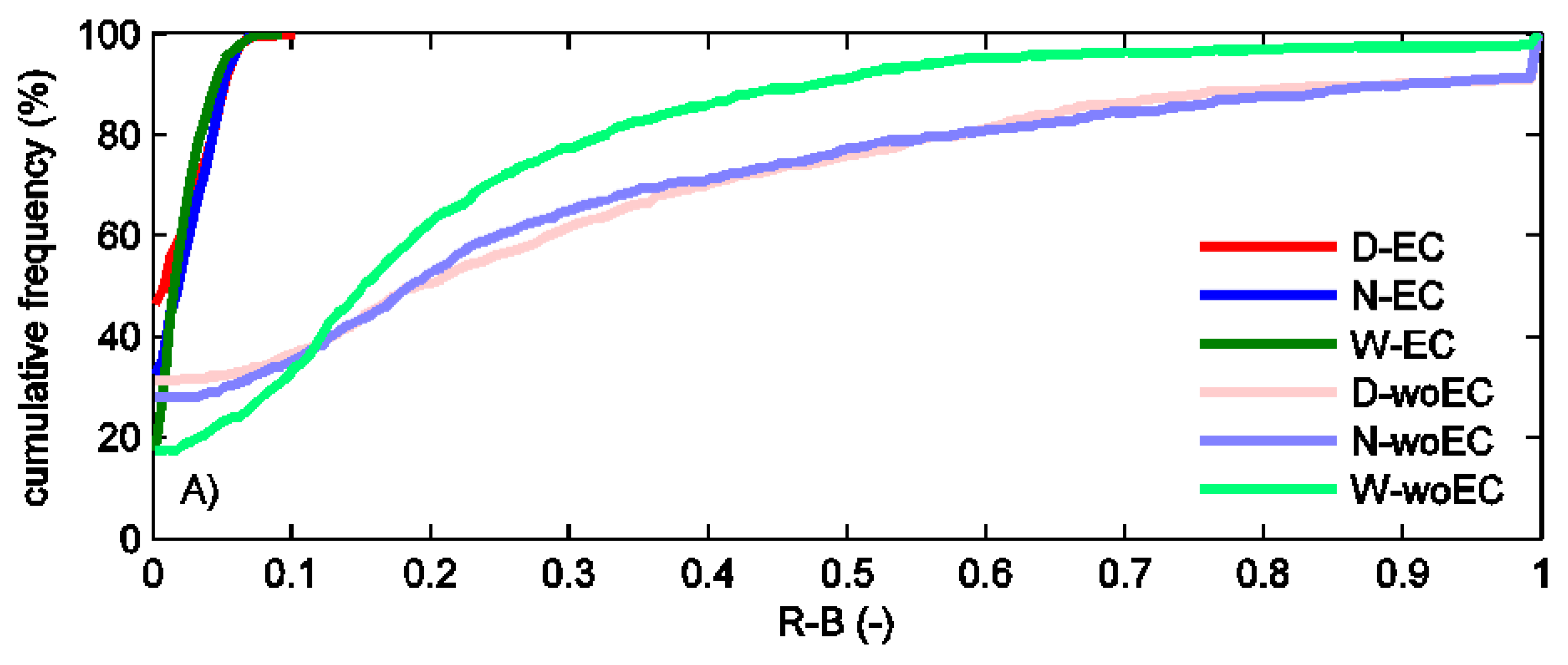
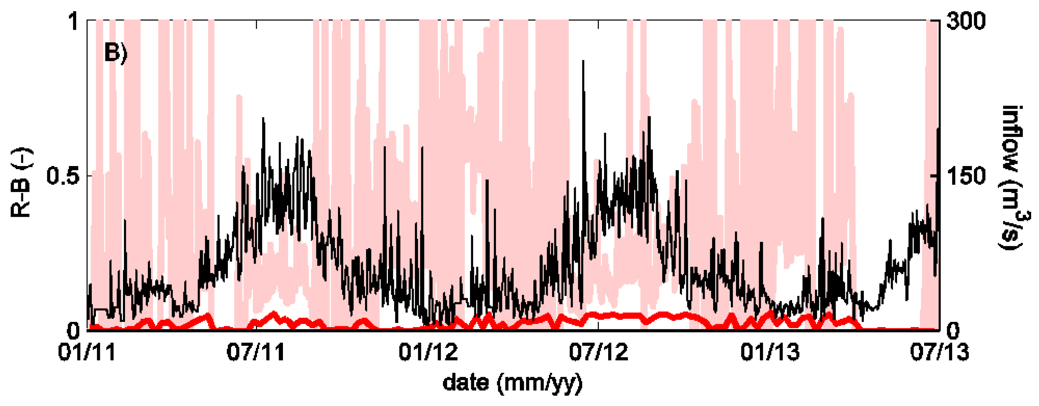
3.4.1. Sub-Daily Hydrologic Alteration

Measuring hydrologic alteration has been of interest since the 1990s. Most well-known are the Indicators of Hydrologic Alteration by Richter et al. [32], based on flows of daily (or coarser) resolution. However, with the privatization of the power sector and the introduction of renewables, the operational scheme of hydropower plants has intensified its flashiness, especially in the intra-daily time horizon [5,33]. These fluctuations are hardly captured in the original indicators [34]. In response, several indexes for measuring the hourly fluctuation have been proposed in the last decade [35,36,37]. The Richard–Baker (R–B) index [35] for flow flashiness is one that has found numerous applications in the last five years [5,6,12,38,39]:
R B   Index =   1 2 t = 1 N 1 ( | q t + 1 q t | + | q t q t 1 | ) t = 1 N q t
where q t denotes the outflow for the time t, and N is the total number time steps used for computing the R–B index. Here we computed the weekly R–B index such that N = 168 because the outflows are obtained every 1 h. The structure of the R–B index is simple and allows to capture the frequency and magnitude of multiple peaking events during the time horizon. It consists of adding the hourly flow variations and dividing them by the total flow of the considered period (e.g., day or year). The coefficient 1/2 restricts the value of the R-B index between 0 and 1. Values close to zero describe very steady flows. An index close to one is the other extreme in which a power plant generates pulses (0% in one hour, 100% in the next, then 0%, and so on) during the whole time horizon.

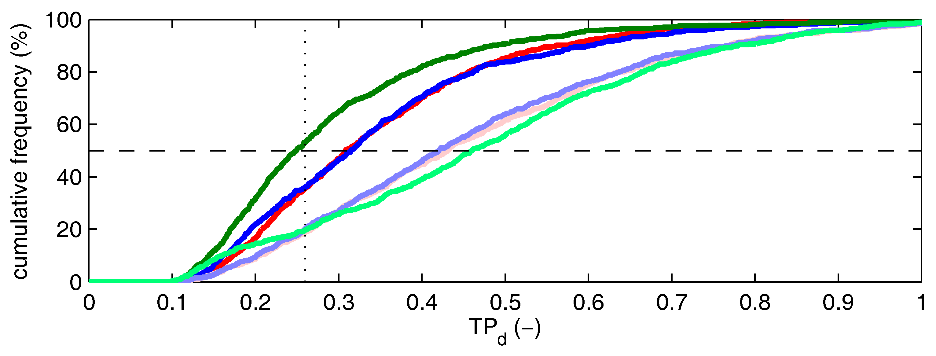
3.4.2. Thermal Pollution

Although water temperature is a central ecological controller, it is rarely considered when defining environmental flow requirements in hydropower reservoirs. Some recent studies have started to focus on this phenomenon [14,40,41]. In [14], the thermal pollution of a hydroelectric dam is characterized in terms of variability and magnitude (monthly range, minima, and maxima) of water temperature, frequency and duration of low and high-temperature pulses that also propagate downstream as thermal plumes [40,41], and timing of yearly minima and maxima temperatures. These analyses compare the conditions before (using the inflow water temperatures) and after the dam construction. In short, the approach is similar to the range of variability approach (RVA) of flows [42].
Vanzo et al. [43] point out that the sub-daily temperatures cycles also impact the ecosystems, but these are hardly captured in the indexes of daily (or coarser) resolution. Consequently, they derived the T P d index for the day d, defined as:
T P d = max | T t + 1 T t | T max d T min d
where T t denotes the outflow water temperature for the time t, and T max d and T min d , the maximum and minimum outflow temperature, respectively, for the day d. T P d is a dimensionless index that measures the rate of change of temperature over short time scales with respect to the difference between the maximum and minimum temperature of that day d. The index ranges between 0 and 1, where values close to zero indicate smooth temperature changes, while T P d closer to 1 indicates high thermal alteration in the downstream river.
Finally, the outflow water temperature is computed as the average water temperature of the reservoir, for the boundary cells near of the dam located between 73 and 88 m.a.s.l.

3.4.3. Vertical Mixing

Changes in outflow water temperature with respect to the inflow water temperature and changes in the sub-daily thermal regime are driven by the hydrodynamics of the reservoir. Hence, we will focus on variations in the vertical stratification that reflect the rate at which mixing occurs across the density interface, thus transporting water constituents (like nutrients or biochemical oxygen demand) from the hypolimnion to the epilimnion. To quantify changes in the stratification, we looked at the potential energy of the reservoir, PE , computed along the longitudinal curtain (marked in Figure 1) as:
PE = Ω 0 H ρ g z d z d Ω
where ρ denotes the water density, g the gravity acceleration, z the elevation and Ω the surface area of the integration. The potential energy is smaller for stratified conditions than for well-mixed conditions [44,45,46]. Consequently, with Equation (4) we computed the difference between PE of the well-mixed reservoir and PE of the stratified reservoir for each time step, where for the former we used the spatial average of the water density. This difference is here called Δ P E , and is a time series that defines the amount of energy that is required to produce the complete vertical mixing in the reservoir. Consequently, smaller values of Δ P E are associated to a more mixed water column. Finally, to explain the differences among time series of Δ P E of the different scenarios, the kinetic energy of the reservoir, KE, was computed as:
KE = Ω 0 H ρ ( v · v ) 2   d z d Ω
where v denotes the simulated flow velocity.

4. Results and Discussion

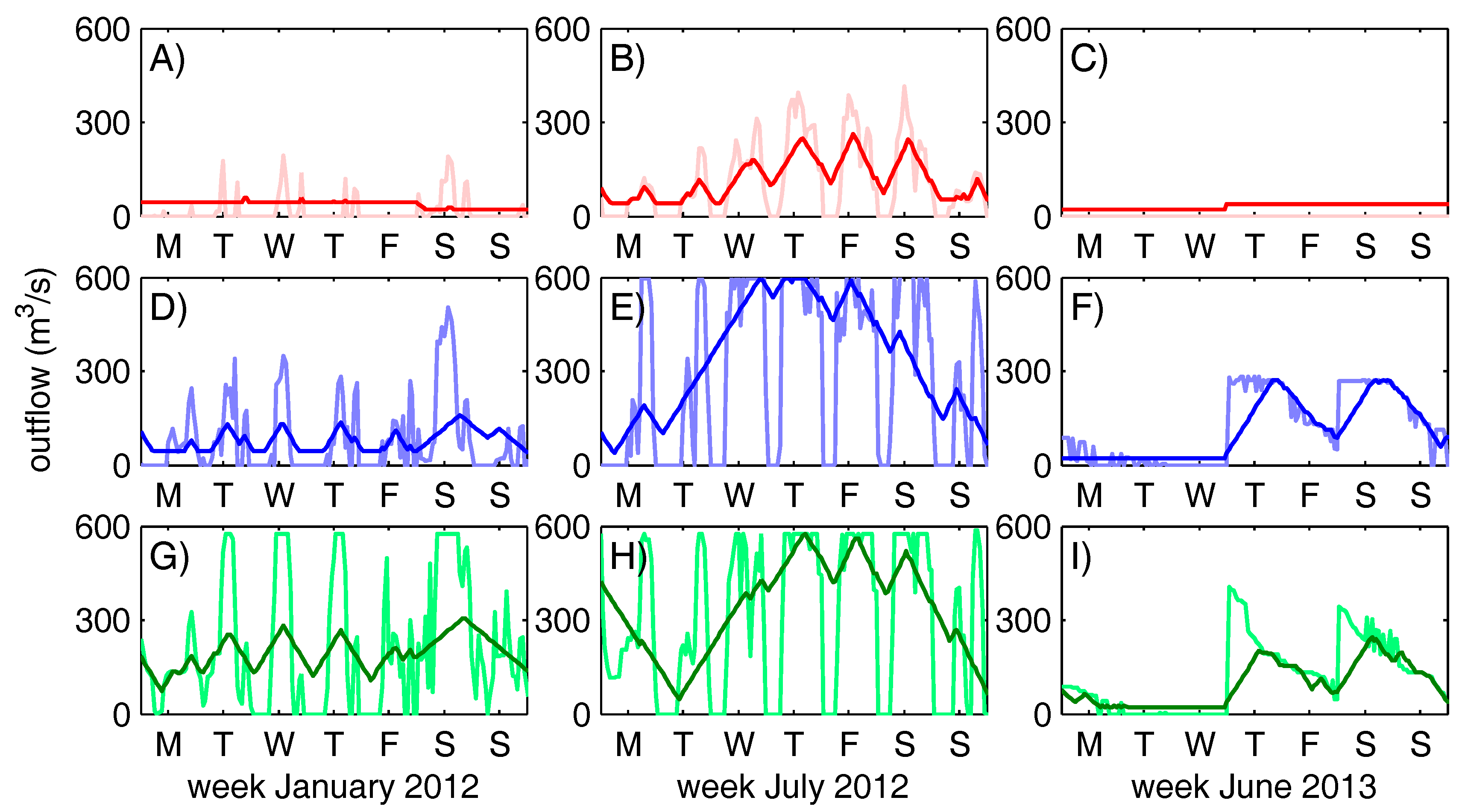
4.1. Power System Operations Simulation

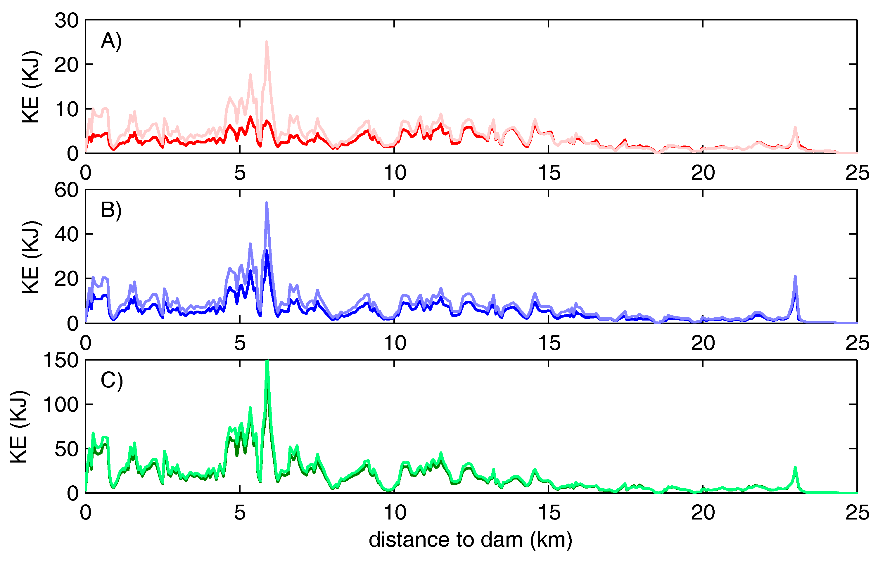
4.1.1. Sub-Daily Hydrologic Alteration

The main results of power system operations simulation with MIP-UC, related to the operation of the Rapel hydropower plant, are shown in Figure 3. For different weeks and hydrologic scenarios, it compares the flow between the scenario with EC (dark lines) and without EC (light lines). The EC included in this study limit these fluctuations and force the hydropower plant to a smoother operation during the entire simulation period.
As expected by design, the R-B flashiness index is effectively reduced when EC are considered (see also, for example, Figure 4A and reference [12]). Furthermore, the R–B index showed smaller values for the W-woEC (light green line) scenario than for the D- and N-woEC scenarios (Figure 4A), which shows that hydropeaking in wet conditions is less intense than for normal and dry scenarios. This can be attributed to the lack of water availability in the D- and N- scenarios in contrast to the W scenario. Finally, on the seasonal evolution of the flashiness, Figure 4B compares time series of the flashiness index for a dry hydrology of the scenarios with and without EC. It shows that the scenario without EC (light red line) has low R-B values for larger inflows (austral winter), while it peaks during summer where the inflows are small. This relationship is observed for all the scenarios without EC.

4.1.2. Costs of EC

The implementation of ECs raises the annual costs by 5 to 22 million USD (shown in Table 2), as computed by grid-wide power operations model, depending on the hydrologic scenario. In terms of direct costs of the Rapel reservoir, Table 2 shows that the implementation of ECs raises annual costs US$2.2 to 8.8 million (shown in Table 2), corresponding to a relative increase in annual costs by 3.9% to 10.9%. As it is shown in Table 2, this cost increase might be relevant for a single power plant but corresponds to less than a 0.3% system-wide cost increase. The system-wide costs are considered relevant because these are finally transmitted to the customers. This growth is considerably low, especially in the context of the cost variability due to hydrologic scenarios. For example, a normal year is 6% more expensive than a wet year, and a dry year is over 12% more costly than a normal year.
The relatively low cost of implementing ECs in dry years might seem counter-intuitive. This can be explained by the effect that water scarcity has on the generation mix. In these years, there is a high participation of thermal power plants, which offer peaking capacity. Therefore, the lost ramping capacity from a constrained hydropower operation can easily be distributed among the (many) available thermal units. In normal and wet years, in contrast, limiting the hydropower operation would imply using expensive thermal-peakers that otherwise would remain off.
There is a trade-off between the costs and the benefits associated with the inclusion of ECs on the operation of the hydropower plant. These costs are explicitly calculated as the grid-wide cost increases (monetary costs of Table 2), whereas the benefits associated with hydrologic and thermal alteration of the downstream river, and vertical mixing in the reservoir are expressed in non-monetary indexes. So far, our analysis treats the environmental benefits in a different dimension as the economic costs. In future, it would be helpful to advance in the economic understanding of these benefits for an optimal design of ECs.

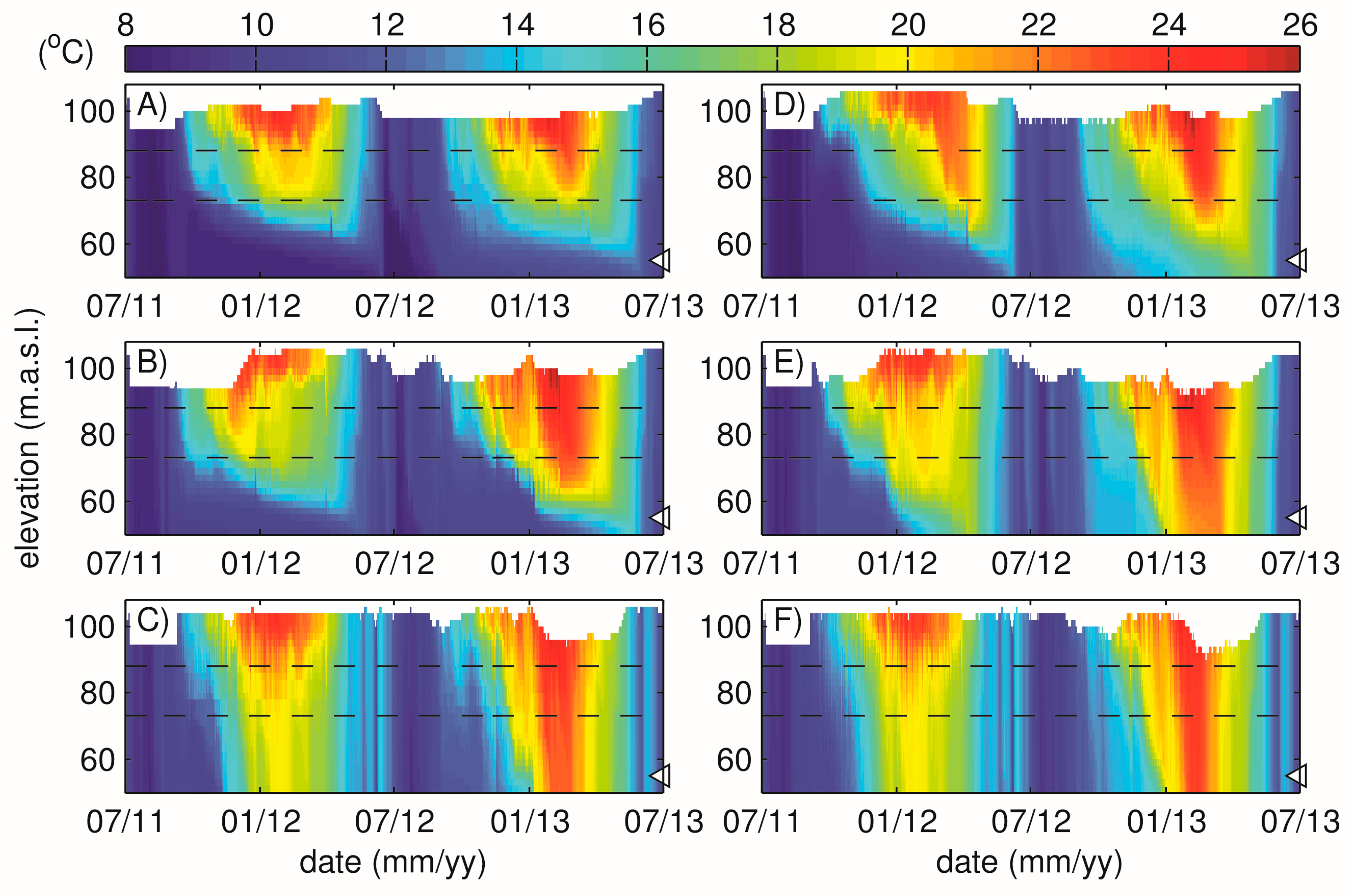
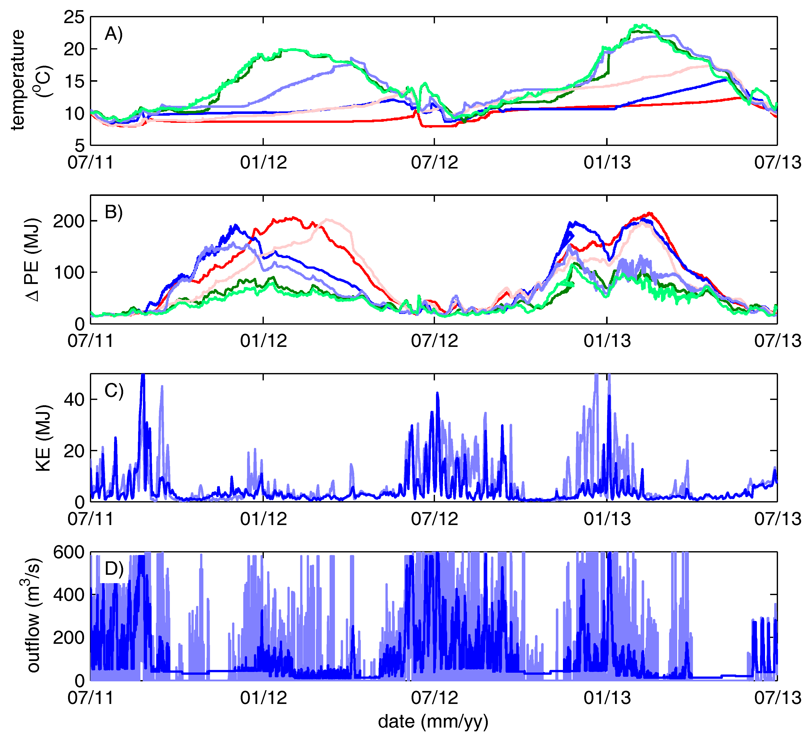
4.2. Water Temperature

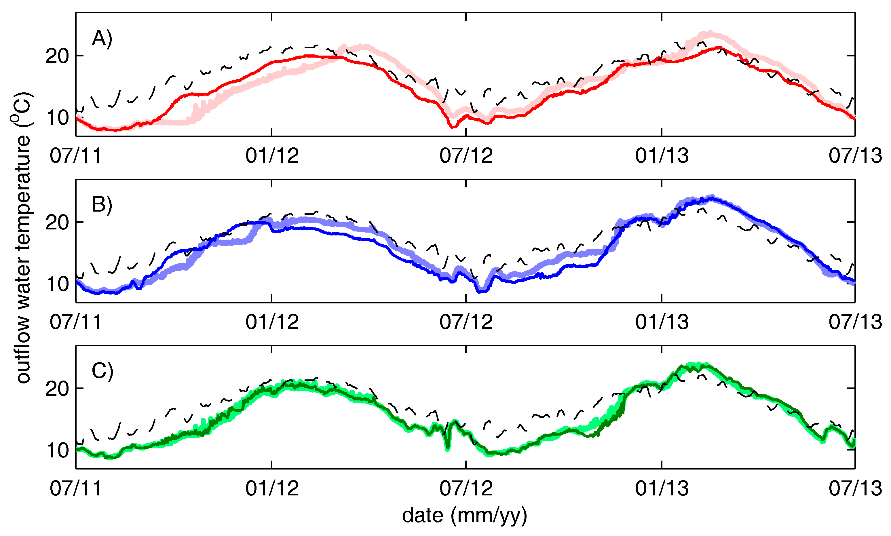
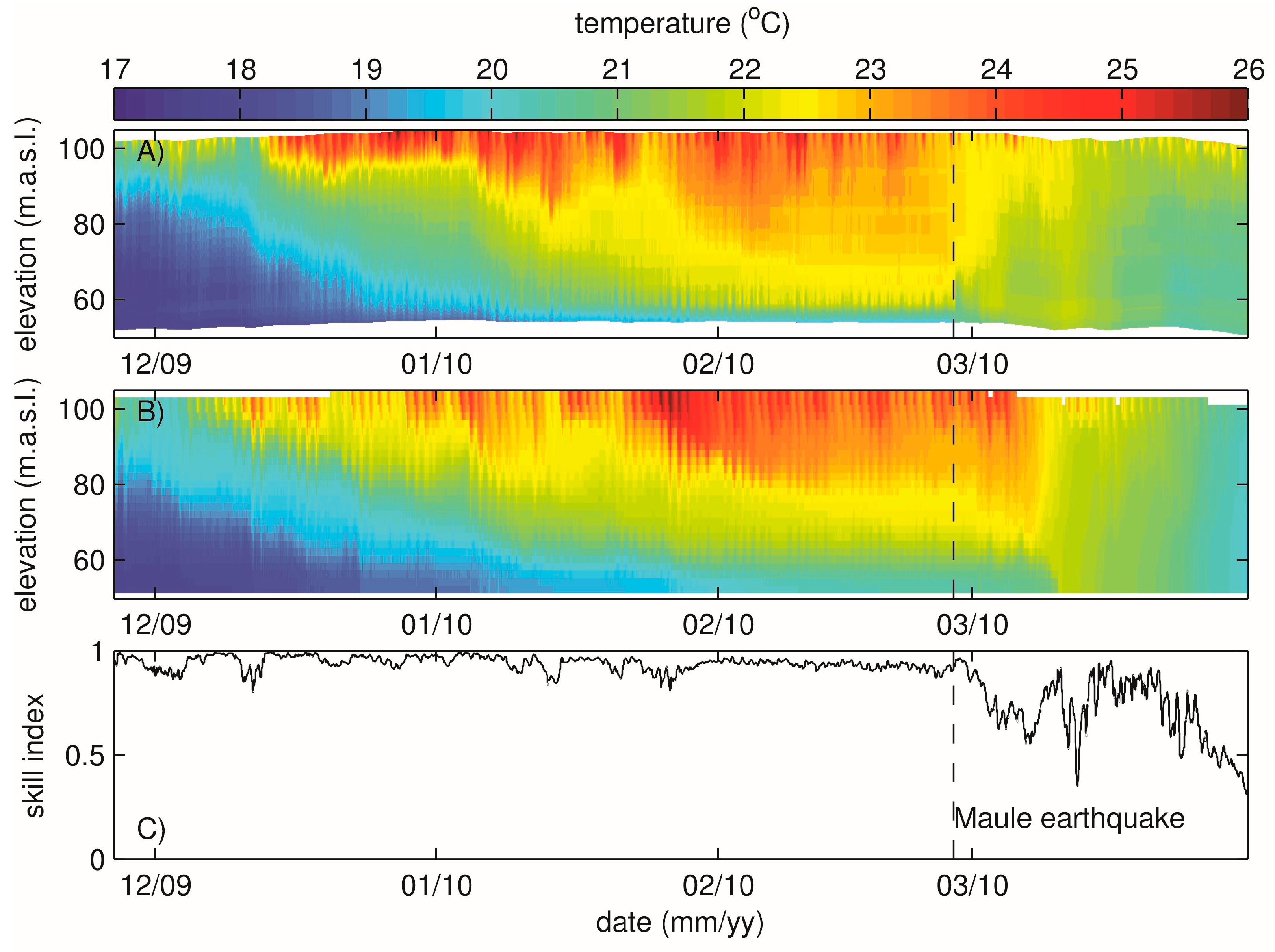
4.2.1. Water Temperature Validation

The direct comparison between observed (thermistor chain) and simulated (ELCOM) vertical profiles of water temperature near the dam is shown in Figure 5A,B, respectively. The performance of the model (Figure 5C) is favorable most of the time as the skill index takes values larger than 0.9 during most part of the time. Only after the end of February 2010, the skill index value starts to decrease, due to the Mw8.8 Maule earthquake that produced an intense and instantaneous vertical mixing in Rapel reservoir [24], which is not represented in the hydrodynamic model. The skill index plotted in Figure 5C was computed based on Equation (1) with the observed and predicted water temperatures plotted in Figure 5A,B, respectively. Unfortunately, no other water temperature measurements are available for this validation period to evaluate the performance of the model in other places of the reservoir.

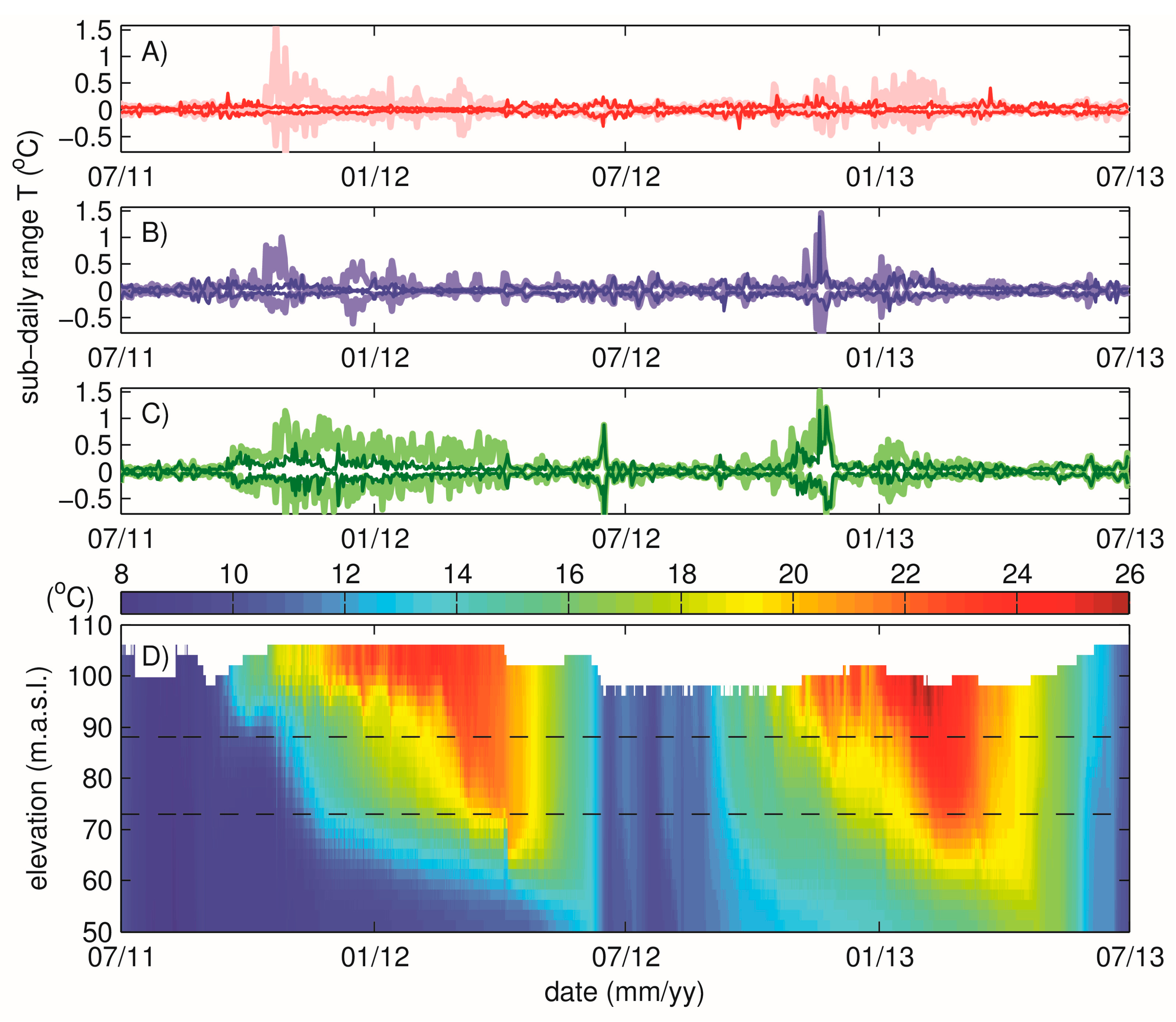
4.2.2. Vertical Mixing in the Rapel Reservoir

The hydrodynamics simulations show substantial differences in water temperature as a function of the presence of ECs and the hydrologic regime. Figure 6 shows the time evolution of vertical profiles of water temperature near the dam (this profile determines the downstream water temperature). As previously reported, the location of the density interface is primarily determined by the elevation at which the outlet is installed (between 73 and 88 m.a.s.l., see the horizontal dashed lines in Figure 6). However, the vertical profiles of water temperature are also determined by both the hydrology and the presence of ECs. As a consequence, dry scenarios with smaller outflow volumes (Figure 6C,D) are less well mixed than wet scenarios (Figure 6C,F) associated with higher outflows.
The impact of the ECs on the hydrodynamics of the reservoir can be observed in Figure 7A, where the time series of water temperature at 20 m below the water outlet elevation (triangles of Figure 6) are plotted for all the simulated scenarios. The dry years without ECs show the lowest water temperatures and no significant seasonal changes, while the water temperature for the wet year shows a strong seasonal signal with maximum values of 22 °C. This response evidences the fact that vertical mixing across the density interface is weakest for the D-EC scenario. Here, the deep water temperature was determined by the reservoir temperature in the previous winter turnover, rather than by seasonal cycles that control surface temperature. Figure 7A also shows that the inclusion of ECs may imply less vertical mixing and thus lower water temperatures.
In terms of potential energy, Figure 7B shows the time series of the energy required to completely mix the water column ( Δ PE ). This is a way of quantifying the stratification of the water column (Figure 6). As expected, Δ PE is larger during summer in all the simulations when the water column is stratified, i.e., a large amount of energy is required to produce vertical mixing. Furthermore, Δ PE is consistently larger when EC are in place. In extreme cases, the Δ PE of scenarios with ECs can double the Δ PE of scenarios without ECs (e.g., normal hydrologic years during the second summer). Finally, the hydrology also plays an important role in vertical mixing. The Δ PE of wet years is smaller in normal than in dry years. Moreover, during a wet year ECs have no significant impact on Δ PE .
The link between vertical mixing, the hydrology, and the hydropower plant operation is better observed by looking at the kinetic energy of the reservoir (Figure 7C) in response to the outflows (Figure 7D). Two facts are highlighted: (1) the comparison between outflows and KE time series shows that the kinetic energy of the reservoir is well modulated by outflows, such that KE is maximum when outflow discharges occurs; and (2) similarly to Ibarra and colleagues [21] (which looked at the mixing efficiency to quantify vertical mixing in response to the outflows and the wind), the KE for the normal scenario without ECs is usually larger than the KE with ECs. The latter is because of the kinetic energy is proportional to the square of the velocity, which is larger for scenarios without ECs than with ECs, which tend to smooth the outflow time-series [21]. In response to these two facts, the KE available for mixing the reservoir is smaller for the dry hydrology than for the wet hydrology (the average KE for the for D-, N-, and W-EC scenarios is 2.8, 4.5 and 15.3 MJ, respectively), and the KE takes larger values for scenarios without ECs (3.4, 6.5 and 17.6 MJ, for D-, N-, and W-woEC scenarios, respectively).
Finally, this increase in the KE available to produce mixing is restricted to the Muro basin as shown in Figure 8, which plots the temporal average KE computed for all of the computational cells of that define the longitudinal curtain defined in the red line of Figure 1. Particularly, the KE associated with the woEC scenarios (light lines in Figure 8) is generally higher that the KE of the EC scenarios for the region between the dam and the kilometer 15 of the longitudinal curtain, which is located downstream the confluence of Cachapoal and Alhué basins (Figure 1). Furthermore, an interesting feature is also observed in Figure 8 at km 6, where the KE of all the simulations was maxima. This localized increase in the KE is because of a lateral contraction of the bathymetry (see Figure 1) which locally enhances the flow velocity. Notice that vertical axis limits of subplots of Figure 8 are not the same, such that the KE for wet scenarios (Figure 8C) is twice as large than KE for normal scenarios (Figure 8B), and five times larger than the KE simulated for dry scenarios.

4.2.3. Thermal Alteration of the Downstream River

The downstream river temperature is modulated by the water temperature of the reservoir in both the seasonal and the sub-daily timescales. For the seasonal time-scale, Figure 9 shows the time series of inflow and outflow water temperatures for the different scenarios. Usually, the outflow water temperature of Rapel is lower than the inflow water temperature (Figure 9A–C). This can be explained by the deep-water intakes, areas colder than the surface. Furthermore, the average outflow water temperature depends on the ECs. In particular, the average outflow temperature without EC is about 0.4 °C higher for dry and normal years when compared to the cases with ECs. For the wet hydrology, the difference is negligible. However, for normal and dry years, the inclusion of ECs could produce differences in the outflow temperature as large as 2 to 3 °C (both positive and negative).
On the sub-daily time-scale, hydropeaking generates significant fluctuations in the outflow water temperature. However, these oscillations can be effectively dampened with ECs. This can be observed in Figure 10A–C that plot the time series of sub-daily anomalies of outflow water temperature (maximum daily temperature minus daily average temperature, and maximum daily temperature minus daily average temperature). As found in [21], the large fluctuations in the outflow water temperature associated with the woEC scenarios are explained by the outflows discharge pulses that pull (warmer) water from the surface. Consequently, sub-daily temperature anomalies are larger at the beginning of the stratification period. Here, the stratification starts to build up from the top, and the vertical gradients of water temperature are greater than at the end of the summer. Furthermore, positive sub-daily anomalies of outflow water temperature are larger than negative anomalies, which confirm that hydropeaking draws from warmer waters. Finally, the simulations with ECs showed smaller fluctuations in the outflow water temperatures than for the woEC scenarios. The daily fluctuations in the outflow temperature of the EC scenarios are attributed to diurnal cycles of water temperature and to the fact that some peaking is allowed by the MRR restriction.
Finally, for quantifying sub-daily thermal alteration in the downstream river, Figure 11 plots the cumulative frequencies associated to the T P d index of reference [43] (Equation (3)). The authors of [43] used the median value of the station and defined the threshold T P d = 0.26 to indicate whether or not the thermal alteration is substantial (dashed line in Figure 11). In the Rapel reservoir, the computed T P d index is, in general, larger than this threshold, thus indicating that the sub-daily thermal alteration of the downstream river is significant.

5. Conclusions

In this paper we couple a power system scheduling model to a hydrodynamic simulation to study the effects of the operation of a hydropower plant on water temperature, hydrological alteration and vertical mixing in the reservoir. We focus on sub-daily hydrologic alteration, seasonal and sub-daily thermal pollution and vertical mixing. Further, we assess how environmental constraints (ECs) affect these parameters and how much these ECs would cost. We present a case study in Chile (Rapel hydropower plant) and test the results for robustness under three different water-type years (wet, normal and dry).
In quantitative terms, the impacts of the implementation of ECs on the operation of Rapel hydropower plant are summarized in Table 3. It shows the relative changes of implementing ECs in terms of monetary cost, hydrological and thermal alteration, and vertical stratification. We found that Rapel’s current (unconstrained) operation induces a strong sub-daily hydrologic alteration of the downstream river. The implementation of ECs would reduce this to a large extent. Particularly, extreme peaking events would be avoided. Furthermore, the operation of the power plant also generates significant fluctuations in the outflow water temperature on the seasonal and sub-daily time-scale. Here, the implementation of ECs also dampens these fluctuations. Further, on the seasonal scale, ECs can help lowering the river’s temperature. The current (unconstrained) operation promotes vertical mixing, especially critical in summer when algae blooms are frequent. Implementing ECs might strengthen the seasonal stratification close to the dam in summer, particularly during dry and normal years. Once ECs are implemented, the system-wide operational costs are expected to increase by about 0.3%. From a systemic perspective, this does not seem significant. However, if the power plant needs to bear them, it could have noticeable effects on its yearly balance.
In summary, the inclusion of ECs in the operation of the hydropower plant reduces hydrological and thermal alteration of the downstream river. However, it also might strengthen stratification in the Muro basin, which may not necessarily be good for the water quality of the reservoir.

Acknowledgments

The authors thank the support of the Chilean Council of Scientific and Technological Research (CONICYT/ FONDECYT/1151438, 1140821) and the German Academic Exchange Service (DAAD). Further, we thank Carlos Benavides of the Energy Center of the University of Chile for the development of the unit commitment tool (MIP-UC) and Abel Quintero for processing the hydrologic input data.

Author Contributions

Diego Carpentier prepared and conducted all hydrodynamics and power system operations simulations. Diego Carpentier and Alberto de la Fuente conceived and designed the hydrodynamics simulations, while Jannik Haas and Marcelo Olivares conceived and designed the power system operations simulations. All the authors contributed to analyzing the results and writing the paper.

Conflicts of Interest

The authors declare no conflict of interest.

References

  1. Jager, H.I.; Smith, B.T. Sustainable reservoir operation: Can we generate hydropower and preserve ecosystem values? River Res. Appl. 2008, 24, 340–352. [Google Scholar] [CrossRef]
  2. Hunter, M.A. Hydropower Flow Fluctuations and Salmonids: A Review of the Biological Effects, Mechanical Causes, and Options for Mitigation; Technical Report 119; State of Washington, Department of Fisheries: Olympia, WA, USA, 1992.
  3. Richter, B.D.; Thomas, G.A. Restoring Environmental Flows by Modifying Dam Operations. Ecol. Soc. 2007, 12, 12. [Google Scholar] [CrossRef]
  4. Scheidegger, K.J.; Bain, M.B. Larval Fish Distribution and Microhabitat Use in Free-Flowing and Regulated Rivers. Copeia 1995, 1995, 125–135. [Google Scholar] [CrossRef]
  5. Haas, J.; Olivares, M.A.; Palma-Behnke, R. Grid-wide subdaily hydrologic alteration under massive wind power penetration in Chile. J. Environ. Manag. 2015, 154, 183–189. [Google Scholar] [CrossRef] [PubMed]
  6. Kern, J.D.; Patino-Echeverri, D.; Characklis, G.W. The impacts of wind power integration on sub-daily variation in river flows downstream of hydroelectric dams. Environ. Sci. Technol. 2014, 48, 9844–9851. [Google Scholar] [CrossRef] [PubMed]
  7. Kern, J.D.; Characklis, G.W.; Doyle, M.W.; Blumsack, S.; Whisnant, R.B. Influence of Deregulated Electricity Markets on Hydropower Generation and Downstream Flow Regime. J. Water Resour. Plan. Manag. 2012, 138, 342–355. [Google Scholar] [CrossRef]
  8. Poff, N.L.; Allan, J.D.; Bain, M.B.; Karr, J.R.; Prestegaard, K.L.; Richter, B.D.; Sparks, R.E.; Stromberg, J.C. The Natural Flow Regime. Bioscience 1997, 47, 769–784. [Google Scholar] [CrossRef]
  9. Poff, N.L.; Zimmerman, J.K.H. Ecological responses to altered flow regimes: A literature review to inform the science and management of environmental flows. Freshw. Biol. 2010, 55, 194–205. [Google Scholar] [CrossRef]
  10. Bunn, S.E.; Arthington, A.H. Basic Principles and Ecological Consequences of Altered Flow Regimes for Aquatic Biodiversity. Environ. Manag. 2002, 30, 492–507. [Google Scholar] [CrossRef]
  11. Angus Webb, J.; Miller, K.A.; King, E.L.; de Little, S.C.; Stewardson, M.J.; Zimmerman, J.K.H.; LeRoy Poff, N. Squeezing the most out of existing literature: A systematic re-analysis of published evidence on ecological responses to altered flows. Freshw. Biol. 2013, 58, 2439–2451. [Google Scholar] [CrossRef]
  12. Olivares, M.A.; Haas, J.; Palma-Behnke, R.; Benavides, C. A framework to identify Pareto-efficient subdaily environmental flow constraints on hydropower reservoirs using a grid-wide power dispatch model. Water Resour. Res. 2015, 51, 3664–3680. [Google Scholar] [CrossRef]
  13. Pérez-Díaz, J.I.; Wilhelmi, J. Assessment of the economic impact of environmental constraints on short-term hydropower plant operation. Energy Policy 2010, 38, 7960–7970. [Google Scholar] [CrossRef]
  14. Olden, J.D.; Naiman, R.J. Incorporating thermal regimes into environmental flows assessments: Modifying dam operations to restore freshwater ecosystem integrity. Freshw. Biol. 2010, 55, 86–107. [Google Scholar] [CrossRef]
  15. Caissie, D. The thermal regime of rivers: A review. Freshw. Biol. 2006, 51, 1389–1406. [Google Scholar] [CrossRef]
  16. Poole, G.C.; Berman, C.H. An ecological perspective on in-stream temperature: Natural heat dynamics and mechanisms of human-caused thermal degradation. Environ. Manag. 2001, 27, 787–802. [Google Scholar] [CrossRef]
  17. Miara, A.; Tarr, C.; Spellman, R.; Vörösmarty, C.J.; Macknick, J.E. The power of efficiency: Optimizing environmental and social benefits through demand-side-management. Energy 2014, 76, 502–512. [Google Scholar] [CrossRef]
  18. Fischer, H.; List, R.; Imberger, J.; Brooks, N. Mixing in Island and Coastal Waters; Academic Press, inc. Harcourt Brace Jovanovich Publishers: San Diego, CA, USA, 1979. [Google Scholar]
  19. Casamitjana, X.; Serra, T.; Colomer, J.; Baserba, C.; Pérez-Losada, J. Effects of the water withdrawal in the stratification patterns of a reservoir. Hydrobiologia 2003, 504, 21–28. [Google Scholar] [CrossRef]
  20. De la Fuente, A.; Niño, Y. Pseudo 2D ecosystem model for a dendritic reservoir. Ecol. Model. 2008, 213, 389–401. [Google Scholar] [CrossRef]
  21. Ibarra, G.; de la Fuente, A.; Contreras, M. Effects of hydropeaking on the hydrodynamics of a stratified reservoir: The Rapel Reservoir case study. J. Hydraul. Res. 2015, 53, 760–772. [Google Scholar] [CrossRef]
  22. Rossel, V.; de la Fuente, A. Assessing the link between environmental flow, hydropeaking operation and water quality of reservoirs. Ecol. Eng. 2015, 85, 26–38. [Google Scholar] [CrossRef]
  23. Vila, I.; Contreras, M.; Montecino, V.; Pizarro, J.; Adams, D.D. Rapel: A 30 years temperate reservoir. Eutrophication or contamination? Spec. Issues Adv. Limnol. 2000, 55, 31–44. [Google Scholar]
  24. De la Fuente, A.; Meruane, C.; Contreras, M.; Ulloa, H.; Niño, Y. Strong vertical mixing of deep water of a stratified reservoir during the Maule earthquake, central Chile (M w 8.8). Geophys. Res. Lett. 2010, 37. [Google Scholar] [CrossRef]
  25. Centro de Despacho Económico de Carga (Chile’s Power System Operator, CDEC). Data, Statistics and Reports. Available online: http://www.cdec-sing.cl/ (accessed on 12 December 2014).
  26. Chile’s Independent System Operators (CDEC-SING and CDEC-SIC) Statistics of Inflows. Available online: https://sic.coordinadorelectrico.cl/informes-y-documentos/fichas/estadistica-de-caudales-afluentes/ (accessed on 10 October 2016).
  27. Pereira, M.V.F.; Pinto, L.M.V.G. Multi-stage stochastic optimization applied to energy planning. Math. Program. 1991, 52, 359–375. [Google Scholar] [CrossRef]
  28. Chile’s Independent Power System Operator Weekly Scheduling of Chile’s Central Interconnected System. Available online: http://www.cdecsic.cl/informes-y-documentos/fichas/operacion-programada-2/ (accessed on 21 September 2016).
  29. Laval, B.; Imberger, J.; Hodges, B.R.; Stocker, R. Modeling circulation in lakes: Spatial and temporal variations. Limnol. Oceanogr. 2003, 48, 983–994. [Google Scholar] [CrossRef]
  30. Hodges, B.; Imberger, J.; Saggio, A.; Winters, K.B. Modeling Basin-Scale Waves in Stratified Lakes. Limnol. Oceanogr. 2000, 45, 1603–1620. [Google Scholar] [CrossRef]
  31. Willmott, C.J. On the validation of models. Phys. Geogr. 1981, 2, 184–194. [Google Scholar]
  32. Richter, B.; Baumgartner, J.; Powell, J.; Braun, D. A Method for Assessing Hydrologic Alteration within Ecosystems. Conserv. Biol. 1996, 10, 1163–1174. [Google Scholar] [CrossRef]
  33. Kern, J.D.; Patino-Echeverri, D.; Characklis, G.W. An integrated reservoir-power system model for evaluating the impacts of wind integration on hydropower resources. Renew. Energy 2014, 71, 553–562. [Google Scholar] [CrossRef]
  34. Bevelhimer, M.S.; McManamay, R.A.; O’Connor, B. Characterizing sub-daily flow regimes: Implications of hydrologic resolution on ecohydrology studies. River Res. Appl. 2015, 31, 867–879. [Google Scholar] [CrossRef]
  35. Baker, D.B.; Richards, R.P.; Loftus, T.T.; Kramer, J.W. A new flashiness index: Charactersitics and applications to midwestern rivers and streams. J. Am. Water Resour. Assoc. 2004, 40, 503–522. [Google Scholar] [CrossRef]
  36. Lundquist, J.D.; Cayan, D.R. Seasonal and Spatial Patterns in Diurnal Cycles in Streamflow in the Western United States. J. Hydrometeorol. 2002, 3, 591–603. [Google Scholar] [CrossRef]
  37. McKinney, T.; Speas, D.W.; Rogers, R.S.; Persons, W.R. Rainbow Trout in a Regulated River below Glen Canyon Dam, Arizona, following Increased Minimum Flows and Reduced Discharge Variability. N. Am. J. Fish. Manag. 2001, 21, 216–222. [Google Scholar] [CrossRef]
  38. Zimmerman, J.K.H.; Letcher, B.H.; Nislow, K.H.; Lutz, K.A.; Magilligan, F.J. Determining the effects of dams on subdaily variation in river flows at a whole-basin scale. River Res. Appl. 2010, 26, 1246–1260. [Google Scholar] [CrossRef]
  39. Shiau, J.-T.; Wu, F.-C. Optimizing environmental flows for multiple reaches affected by a multipurpose reservoir system in Taiwan: Restoring natural flow regimes at multiple temporal scales. Water Resour. Res. 2013, 49, 565–584. [Google Scholar] [CrossRef]
  40. Webb, B.W.; Hannah, D.M.; Moore, R.D.; Brown, L.E.; Nobilis, F. Recent advances in stream and river temperature research. Hydrol. Process. 2008, 22, 902–918. [Google Scholar] [CrossRef]
  41. Bruno, M.C.; Siviglia, A.; Carolli, M.; Maiolini, B. Multiple drift responses of benthic invertebrates to interacting hydropeaking and thermopeaking waves. Ecohydrology 2013, 6, 511–522. [Google Scholar] [CrossRef]
  42. Richter, B.; Baumgartner, J.; Wigington, R.; Braun, D. How much water does a river need? Freshw. Biol. 1997, 37, 231–249. [Google Scholar] [CrossRef]
  43. Vanzo, D.; Siviglia, A.; Carolli, M.; Zolezzi, G. Characterization of sub-daily thermal regime in alpine rivers: Quantification of alterations induced by hydropeaking. Hydrol. Process. 2016, 30, 1052–1070. [Google Scholar] [CrossRef]
  44. Winters, K.B.; Lombard, P.N.; Riley, J.J.; D’Asaro, E.A. Available potential energy and mixing in density-stratified fluids. J. Fluid Mech. 1995, 289, 115–128. [Google Scholar] [CrossRef]
  45. Antenucci, J.; Imberger, J. Energetics of long internal gravity waves in large lakes. Limnol. Oceanogr. 2001, 46, 1760–1773. [Google Scholar] [CrossRef]
  46. Ulloa, H.N.; Winters, K.B.; de la Fuente, A.; Niño, Y. Degeneration of internal Kelvin waves in a continuous two-layer stratification. J. Fluid Mech. 2015, 777, 68–96. [Google Scholar] [CrossRef]
Figure 1. Bathymetry of the Rapel Reservoir. The red line defines the longitudinal curtain along which the kinetic and potential energy are computed. The black arrows mark two specific locations along the curtain that are used in the discussion. m.a.s.l.: m above sea level.
Water 09 00367 g001
Figure 2. Layout for the coupled simulation of hydrodynamics and operation of the hydropower plant. MIP-UC: mixed integer optimization to prescribe the unit commitment; ELCOM: Estuary, Lake and Coastal Ocean Model.
Water 09 00367 g002
Figure 3. Simulated outflows of Rapel (following the structure of Figure 3) for the different hydrologic scenarios (dry, normal, wet). The color convention is defined in Figure 2. (A,D,G): a specific week of January 2012 (austral summer). (B,E,H): a specific week of July 2012 (austral winter with energy production). (C,F,I): a specific week of June 2013 (austral winter with reduced operation of the hydropower plant).
Water 09 00367 g003
Figure 4. (A) Frequency distribution of Richard-Baker (R-B) index for the scenarios with ECs and without ECs. (B) Time series of R-B index for the simulated outflow time series of the dry scenario with ECs (red line) and without ECs (light red line); the black line indicates the inflows for dry hydrology.
Water 09 00367 g004aWater 09 00367 g004b
Figure 5. Comparison between measured (panel A) and simulated (panel B) water temperature profile near the dam. (C) Time series of the Willmott skill index. Dashed vertical line marks the Maule earthquake.
Water 09 00367 g005
Figure 6. (AC) Time evolution of simulated vertical profiles of water temperature near the dam, for the dry, normal and wet scenario without EC; and (DF) for the dry, normal and wet scenario with EC. Triangles on the right vertical axis indicate location of water temperature time series of Figure 7A, and horizontal dashed lines the elevation of water withdrawals.
Water 09 00367 g006
Figure 7. Time series of: (A) Simulated water temperature at 55 m.a.s.l. (triangles in Figure 6); (B) energy that is required to produce the complete vertical mixing in the reservoir, Δ PE ; (C) kinetic energy, KE, for N-EC and N-woEC scenarios; (D) Simulated outflows for N-EC and N-woEC scenarios. The colors are defined in Figure 2.
Water 09 00367 g007
Figure 8. Temporal averaged KE along the curtain defined in red line of Figure 1. The colors are defined in Figure 2.
Water 09 00367 g008
Figure 9. Time series of simulated daily average inflow water temperature (black dashed line) and daily average outflow water temperature for scenarios with and without ECs. (A) Dry hydrology; (B) normal hydrology and (C) wet hydrology. The colors are defined in Figure 2.
Water 09 00367 g009
Figure 10. Time series of simulated sub-daily anomalies of outflow water temperature (maximum and minimum) for scenarios with and without ECs; and (A) dry hydrology, (B) normal hydrology, and (C) wet hydrology. Colors are defined in Figure 2. (D) Time evolution of simulated vertical profiles of water temperature near the dam for the dry year without ECs. Dashed horizontal lines define the elevation of water withdrawals.
Water 09 00367 g010
Figure 11. Frequency distribution of the sub-daily temperature rate of change index T P d . The colors are defined in Figure 2.
Water 09 00367 g011
Table 1. Scenarios for the power system and hydrodynamics simulations.
EC/HydrologyDryNormalWet
With ECD-ECN-ECW-EC
Without ECD-woECN-woECW-woEC
Table 2. Annual cost increase associated with the inclusion of ECs in terms of system costs, and direct costs of Rapel. Values are presented in terms of % and in millions of US dollars (M USD).
EC-woECDryNormalWet
System costsPercentage (M USD)0.06% (5)0.3% (23)0.3% (22)
Rapel costsPercentage (M USD)3.9% (2.2)10.9% (8.8)6.8% (7.8)
Table 3. Summary of relative changes of the implementation of ECs to Rapel hydropower plant ( EC woEC ) / woEC ) for different aspects analyzed in this article. The quantification was made based on the variable listed in the second column.
AspectVariableDryNormalWet
Monetary costsCost of the power system+0.1%+0.3%+0.3%
Hydrological alterationMedian R-B index−94%−89%−89%
Thermal alterationMedian T P d index−28%−25%−46%
Vertical stratificationAverage Δ P E +14%+29%+9%

