Article

Evaluation and Inter-Comparison of Satellite Soil Moisture Products Using In Situ Observations over Texas, U.S.

1
Cooperative Agricultural Research Center, College of Agriculture and Human Sciences, Prairie View A&M University, Prairie View, TX 77446, USA
2
EDF Renewal Energy, San Diego, CA 92128, USA
3
Department of Chemical and Environmental Engineering, Khalifa University, Masdar Institute of Science and Technology, P.O. Box 54224, Abu Dhabi, UAE
*
Author to whom correspondence should be addressed.
Water 2017, 9(6), 372; https://doi.org/10.3390/w9060372
Submission received: 1 March 2017 / Revised: 10 May 2017 / Accepted: 18 May 2017 / Published: 25 May 2017
(This article belongs to the Special Issue Remote Sensing of Soil Moisture)

Abstract

:
The main goal of this study was to evaluate four major remote sensing soil moisture (SM) products over the state of Texas. These remote sensing products are: (i) the Advanced Microwave Scanning Radiometer—Earth Observing System (AMSR-E) (2002–September 2011); (ii) the Soil Moisture Ocean Salinity system (SMOS, 2010–present); (iii) AMSR2 (2012–present); and (iv) the Soil Moisture Active Passive system (SMAP, 2015–present). The quality of the generated SM data is influenced by the accuracy and precision of the sensors and the retrieval algorithms used in processing raw data. Therefore, it is important to evaluate the quality of these satellite SM products using in situ measurements and/or by inter-comparing their data during overlapping periods. In this study, these two approaches were used where we compared each satellite SM product to in situ soil moisture measurements and we also conducted an inter-comparison of the four satellite SM products at 15 different locations in Texas over six major land cover types (cropland, shrub, grassland, forest, pasture and developed) and eight climate zones along with in situ SM data from 15 Mesonet, USCRN and USDA-NRCS Scan stations. Results show that SM data from SMAP had the best correlation coefficients range from 0.37 to 0.92 with in situ measurements among the four tested satellite surface SM products. On the other hand, SM data from SMOS, AMSR2 and AMSR-E had moderate to low correlation coefficients ranges with in situ data, respectively, from 0.24–0.78, 0.07–0.62 and 0.05–0.52. During the overlapping periods, average root mean square errors (RMSEs) of the correlations between in situ and each satellite data were 0.13 (AMSR-E) and 0.13 (SMOS) cm3/cm3 (2010–2011), 0.16 (AMSR2) and 0.14 (SMOS) cm3/cm3 (2012–2016) and 0.13, 0.16, 0.14 (SMAP, AMSR2, SMOS) cm3/cm3 (2015–2016), respectively. Despite the coarser spatial resolution of all four satellite products (25–36 km), their SM measurements are considered reasonable and can be effectively used for different applications, e.g., flood forecasting, and drought prediction; however, further evaluation of each satellite product is recommended prior to its use in practical applications.

1. Introduction

Soil moisture (SM) controls hydrological, ecological and meteorological processes and plays a critical role in the partitioning of available water and energy exchange among the soil, plant and atmosphere continuum [1,2,3,4]. The SM directly influences the rate of evaporation, groundwater recharge and runoff generation and has an important influence on climate [5,6,7]. The global importance of SM has led to its classification as an essential climate variable (ECV) since 2010 [3,8]. The SM is ranked the second top priority parameter (after precipitation) which is essentially needed and its data have a wide range of applications such as in enhancing weather and climate forecasting, improving agricultural productivity and crop yield predictions, drought and flood monitoring and prediction, disaster and health monitoring and others [9]. Moreover, SM also has an impact on the land–atmosphere fluxes of CO2, CH4 and of N2O, which are important greenhouse gases [3,10].
Soil moisture is highly variable in space and time because of the distribution and characteristics of precipitation, soil texture, vegetation and topography [11,12,13,14]. Also, SM is considered a heterogeneous variable and varies on small scales as per soil drainage patterns and soil characteristics. While satellite measurements can cover relatively larger areas, steep terrain and dense vegetation add complexity to the data. On the other hand, in situ measurements are scarce and cover relatively smaller areas [15]. In situ SM measurements are the main information source to understand the local SM distribution and variability. Due to the wide application of SM data in climatological, agricultural, hydrological, meteorological and ecological communities, several networks have been established to monitor SM throughout the world.
Soil moisture can be measured or estimated in various ways such as through in situ measurements (using ground sensors), satellites (remote sensors) and hydrologic models. However, an integrated approach can overcome the drawbacks of each single method and produce more robust data [16,17]. Although in situ measurements of soil moisture are important to calibrate and validate the satellite and modeled SM estimates, precise validation and/or calibration is only achieved if there are sufficient in situ stations available within a satellite footprint or modeled grid [7,8]. Currently, ground measurements of SM are still sparse both temporally and spatially and have limited coverage globally [8,18,19]. On a global scale, the number of in situ monitoring networks is limited and they primarily cover mid-latitude regions. Therefore, only a few measurements are available in Asia, Africa and South America [8,11].
Currently, microwave remote sensing is widely used in mapping the spatial and temporal distribution of SM on a global scale, and SM data have been made available from various remote sensors from as early as 1979 [16,20,21]. The Scanning Multi-channel Microwave Radiometer (SMMR), launched on the Nimbus-7 satellite, was used to monitor soil moisture from 1979 to 1987 [22,23]. The Special Sensor Microwave Imager (SSM/I) launched on the Defense Meteorological Satellite Program (DMSP) platforms has collected soil moisture data since the first DMSP satellite was launched in 1987 [24]. Similarly, other satellites such as Advanced Microwave Scanning Radiometer (AMSR-E, 2002–2011), AMSR2 (2012–present), Soil Moisture and Ocean Salinity (SMOS, 2010–present) and Soil Moisture Active Passive (SMAP, 2015–present) have made significant contributions in the collection of global soil moisture data at a range of scales (Table 1).
Microwave measurements have the benefit of being unaffected by cloud cover and variable surface solar elimination, but there are other factors such as sensor wave lengths and surface characteristics such as surface roughness, vegetation cover, dielectric constant and topography which can impact these microwave measurements [25,26,27]. Each satellite can monitor SM at specific frequencies or wavelengths (1.4 (L), 6.6 (C1), 6.93 (C2), 10.65 (X) GHz. and higher) and cross the Earth at specific times during their ascending or descending overpasses. The frequency of incident radiation has a direct relationship with the depth of penetration and surface roughness. The L, C and X bandwidths are the most commonly used wavelengths in microwave remote sensing to derive SM, yet each wavelength has its own limit to the depth of penetration and response to the surface roughness. For example, an L-band sensor (SMAP and SMOS) can penetrate leaves and small branches and interact with the soil surface, whereas C and X band sensors (AMSR-E and AMSR2) can only penetrate the top layer of the canopy and they cannot penetrate dense vegetation to reach the soil surface [28].
Soil moisture is generally estimated from satellite data on brightness temperature [29]. The brightness temperature is measured via microwave remote sensing which is a function of physical temperature and emissivity of the surface, which shows a surface temperature can impact on SM quality and retrieval. The satellite SM coverage for a particular location can occur on ascending and/or descending passes on a given day. The satellite SM measurements at the different times of the day in a region can provide different SM measurements [30]. Moreover, land surface heterogeneity can play an important role influencing the quality and quantity of satellite-detected soil moisture.
Numerous evaluation studies have been conducted using in situ measurements and model simulations on regional and global scales [31,32,33]. However, limited studies have been conducted in spatial and temporal heterogeneities in the state of Texas (e.g., [34,35]). Given the region’s physical heterogeneity, it is necessary to evaluate satellite soil moisture products before their use in practical applications in Texas [36] or other places with similar heterogeneity. It is not necessarily the case that satellite SM products that have performed well in one region will perform well in other regions [9]. There are a number of factors which have more impact on one satellite dataset than others for a particular region. It is essential to understand the characteristics of remotely-sensed SM observations for correctly interpreting the observed variations and trends in the SM data.
The main goal of this study was to analyze and evaluate the relative quality of globally available passive satellite SM products and in situ measurements in a diverse climate, land cover and dynamic topography of Texas [37]. This evaluation was very important because this state is very sensitive and vulnerable to climate change due to its heterogeneity of surface characteristics. For example, over the past decades, frequent droughts and floods have occurred in this state, with the most extreme drought in 2011 and severe flooding in 2015 and 2016. Although evaluation of satellite SM products has been done over other locations using single or multiple remotely-sensed products, an evaluation focusing on overlapping duration of satellite data has not been done in the state of Texas. The specific objectives of this study are to: (i) evaluate and compare AMSR-E, SMOS, AMSR2 and SMAP SM products and in situ measurements during the overlapping period over the state of Texas, USA; (ii) identify temporal and spatial trends (2010–2016) of SM using in situ and remotely-sensed observations; and (iii) assess the reliability of the soil moisture products from AMSR-E, SMOS, AMSR2 and SMAP sensors and their variations in diverse land covers and climate zones.

2. Materials and Methods
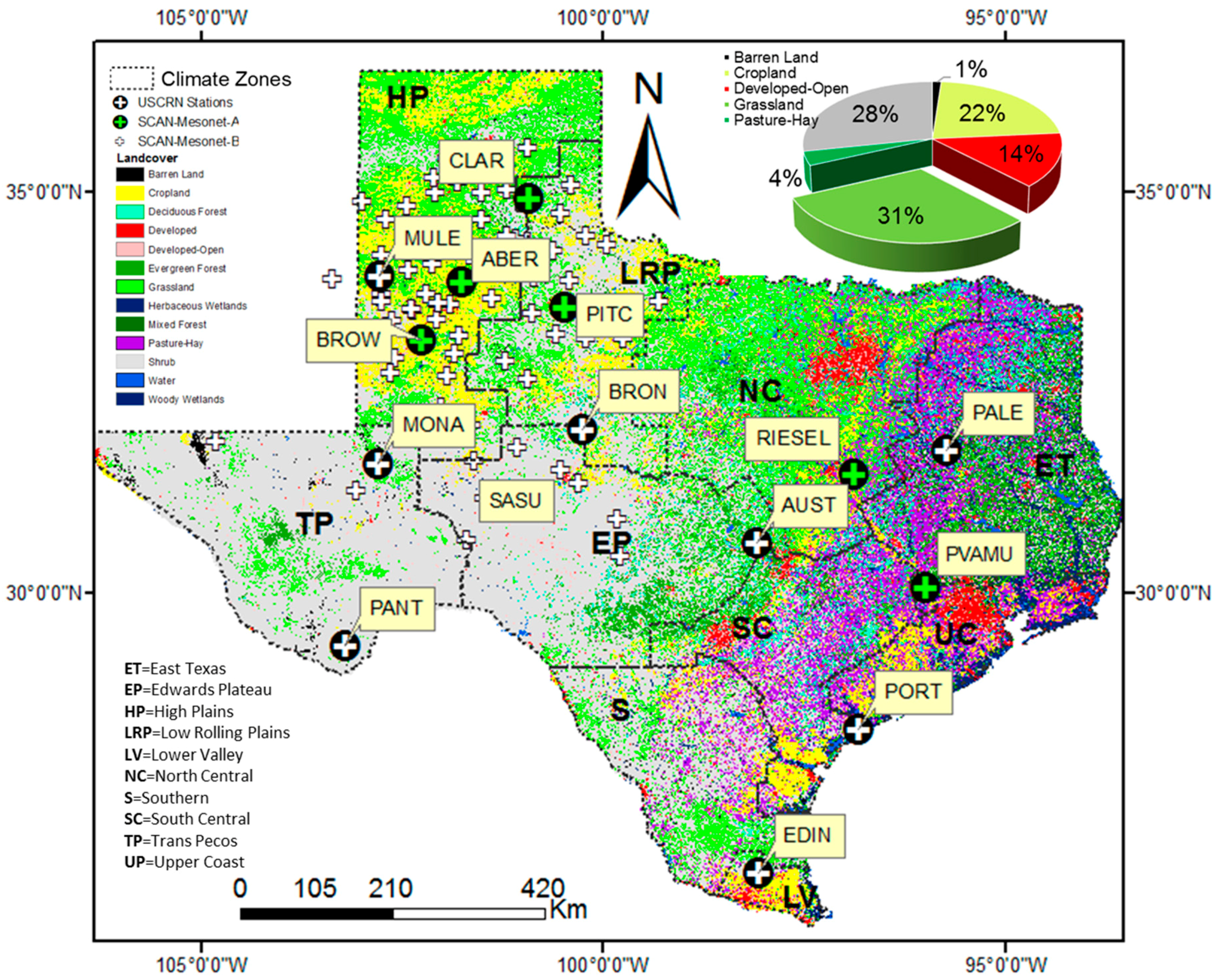
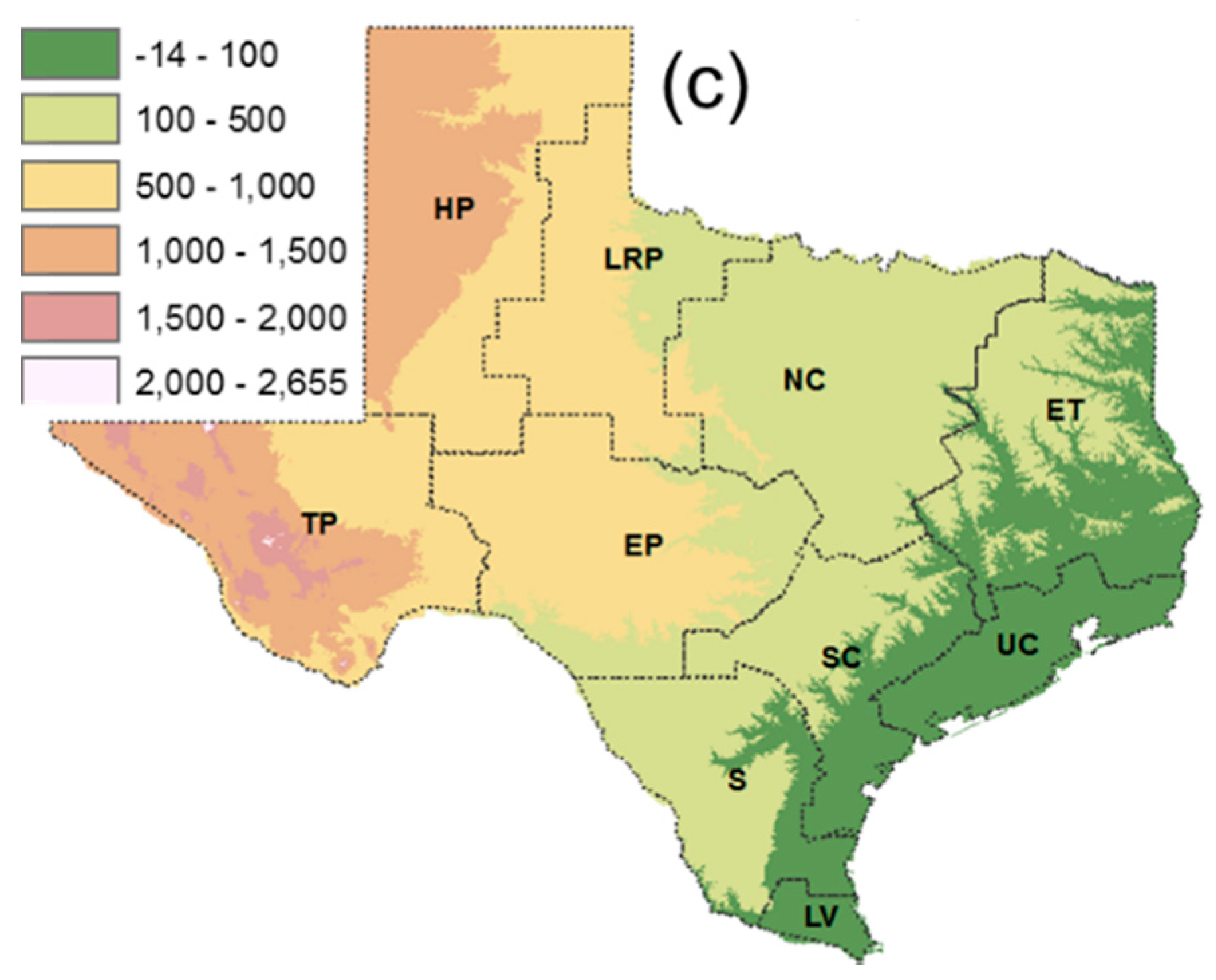
2.1. Study Region

This study was conducted in the state of Texas in the southern US (Figure 1). The climate, geography, land cover and precipitation vary significantly across the state from arid western deserts to humid eastern forests, from sparsely-populated rural regions to the dense metropolitan areas. The distribution of annual average temperature and precipitation suggest a drier south-west and a wetter north-east of the state. The climate of Texas is spatially diverse with ten distinct climatic regions (Figure 2). The state’s climate is unique and complex to understand because it has no dominant climate process governing precipitation in the state [38]. Precipitation varies both spatially and over time. Average annual precipitation increases fairly uniformly from 25 cm in the west to 140 cm in the east with a statewide mean of 70.9 cm/year [39]. It is one of the most rapidly-growing states in the US, with three of the top fastest-growing cities in the country. The fast-growing population is causing a decline in groundwater supplies and is intensifying demands on the limited surface water resources. Texas has an extreme hydrologic variability which includes severe droughts, and diverse climate, geography, economic development, and water management practices [40]. It is dominated by grassland (31%) and shrub land (28%). About 14% of the state is covered by developed-open area and 22% is used for agricultural crops (Figure 1). The state is mostly covered with lower elevation in the south and east and higher elevation in the north and west. The elevation of the state ranges from −14 m in the south to 2655 m in the north. It is dominated by sandy loam (24.5%), loam (20.1%), clay (17.4%) and clay loam (16.3%) surface soil texture whereas sand, loamy sand, silty clay loam and other soil texture only cover 21.7% of the state.

2.2. Remotely-Sensed Data

2.2.1. AMSR-E Soil Moisture

The AMSR-E instrument, developed by the National Space Development Agency of Japan (NASDA), was launched on the Aqua satellite by the National Aeronautics and Space Administration (NASA) on 4 May 2002 [41]. It measures radiation at six frequencies in the range 6.9–89 GHz [34]. Lower frequencies, L-band (1–2 GHz), are more sensitive to soil moisture, but they are more susceptible to dense vegetation and radio frequency interference (RFI). The higher frequency C (6.9 GHz) and X (10.65 GHz) bands can be used to retrieve SM [42] as higher frequency bands are comparatively less susceptible to RFI. A detailed description of the AMSR-E SM retrieval algorithm can be found in [43,44].
This study used the ascending pass (13.30 p.m. local time) AMSR-E SM LPRM level 3 products (X-band) from 1 January 2003, to 31 October 2011, collected on a daily basis. AMSR-E LPRM level 3 products were obtained from NASA Earth Observing System (EOS) Data Gateway through the National Snow and Ice Data Center (NSIDC).

2.2.2. SMOS Soil Moisture

The Soil Moisture and Ocean Salinity (SMOS) satellite mission, from the European Space Agency (ESA), was launched at the end of 2009 and underwent its commissioning phase through May of 2010. During that time frame and extending into the fall of 2010 many changes were made to the algorithms used to determine soil moisture [7]. This satellite carries a microwave synthetic aperture radiometer working at L-band (1.4 GHz).
This study used the daily SM level 3 products from ascending passes (6 a.m.) collected from 2010 to 2016. The SMOS data used to compute level 3 products is the level 2 soil moisture product. To generate SM level 3 products, first, level 2 products were filtered and combined into maps where the spatial resolution was the same as the daily level 2 SMOS product. The SM products are developed by simple spatial averaging at 25 km EASE grid by taking into account only the last orbit measurements in each cell. The required dataset was downloaded from the SMOS Barcelona Expert Center (SMOS-BEC) distribution data website: http://cp34-bec.cmima.csic.es.

2.2.3. AMSR2 Soil Moisture

The Advanced Microwave Scanning Radiometer-2 (AMSR2), developed by the Japanese Aerospace Exploration Agency (JAXA), is a passive microwave radiometer onboard the first Global Change Observation Mission-Water (GCOM-W1) satellite. It was launched in May 2012 and data processing began from July 2012 [45,46,47]. The AMSR2 product is available every 1 to 2 days for ascending (13.30 local time) and descending (1.30 local time) overpasses [45,47]. The Land Parameter Retrieval Model (LPRM) product provides AMSR2 SM retrievals for the 6.9, 7.3 and 10.7 GHz, whereas the JAXA product is only available for 10.7 GHz [48]. This study only used LPRM X-band (10.7 GHz) soil moisture products from ascending overpasses (2012–2016) at a 25-km spatial resolution.

2.2.4. SMAP Soil Moisture

The Soil Moisture Active Passive (SMAP) satellite was launched by NASA on 31 January 2015, to measure SM and freeze/thaw at a global scale using an L-band radiometer and an L-band radar. The SMAP began acquiring routine science data from 31 March 2015 [49]. Currently, SMAP provides data on global SM and freeze/thaw states every 2–3 days using data from an L-band (1.40 GHz.) radiometer only because the SMAP radar stopped transmitting on 7 July 2015 [48]. The SMAP provides SM at a 36-km spatial scale using brightness temperature observations from descending (6 a.m.) passes [50]. The level 3 product is developed using derived geophysical parameters from level 1 or 2 data that have been spatially and/or temporally re-sampled to a global grid. In this study, we re-sampled SMAP 36-km SM data to a 25-km grid in order to make it spatially consistent with other satellite SM products. The product is available from the NASA Distributed Active Archive Center at the NSIDC. This study used SMAP level 3 (SMAP_L3_SM_P) daily SM products from April 2015 to November 2016.

2.2.5. MODIS Data

The Moderate Resolution Imaging Spectro-radiometer (MODIS) instrument, developed by NASA, was launched on the Terra satellite in December 1999 and on the Aqua satellite in May 2002 [51]. MODIS can collect information both in the morning and in the afternoon as Terra is scheduled to pass from north to south across the equator in the morning and Aqua is scheduled to pass from south to north in the afternoon. Even though Terra and Aqua satellites pass in the morning and in the afternoon, respectively, the temporal resolution of MODIS products is only every 1 to 2 days [52]. This data is available at spatial resolutions of 0.25, 0.50, and 1.0 km as well as coarser resolutions [52].
This study used leaf area index (LAI) at a 500-m spatial resolution. The 500-m MODIS LAI (MCD15A3H) product was used to produce spatial maps and temporal distributions of LAI for years 2011 and 2015. The MCD15A3H, 4-day composite LAI values were used in this study. The LAI values were used to study the influence of density of vegetation on soil moisture measurements by four different satellites. These data are available as tiles in the Sinusoidal (SIN) projection. All these data were re-projected into a geographical projection.

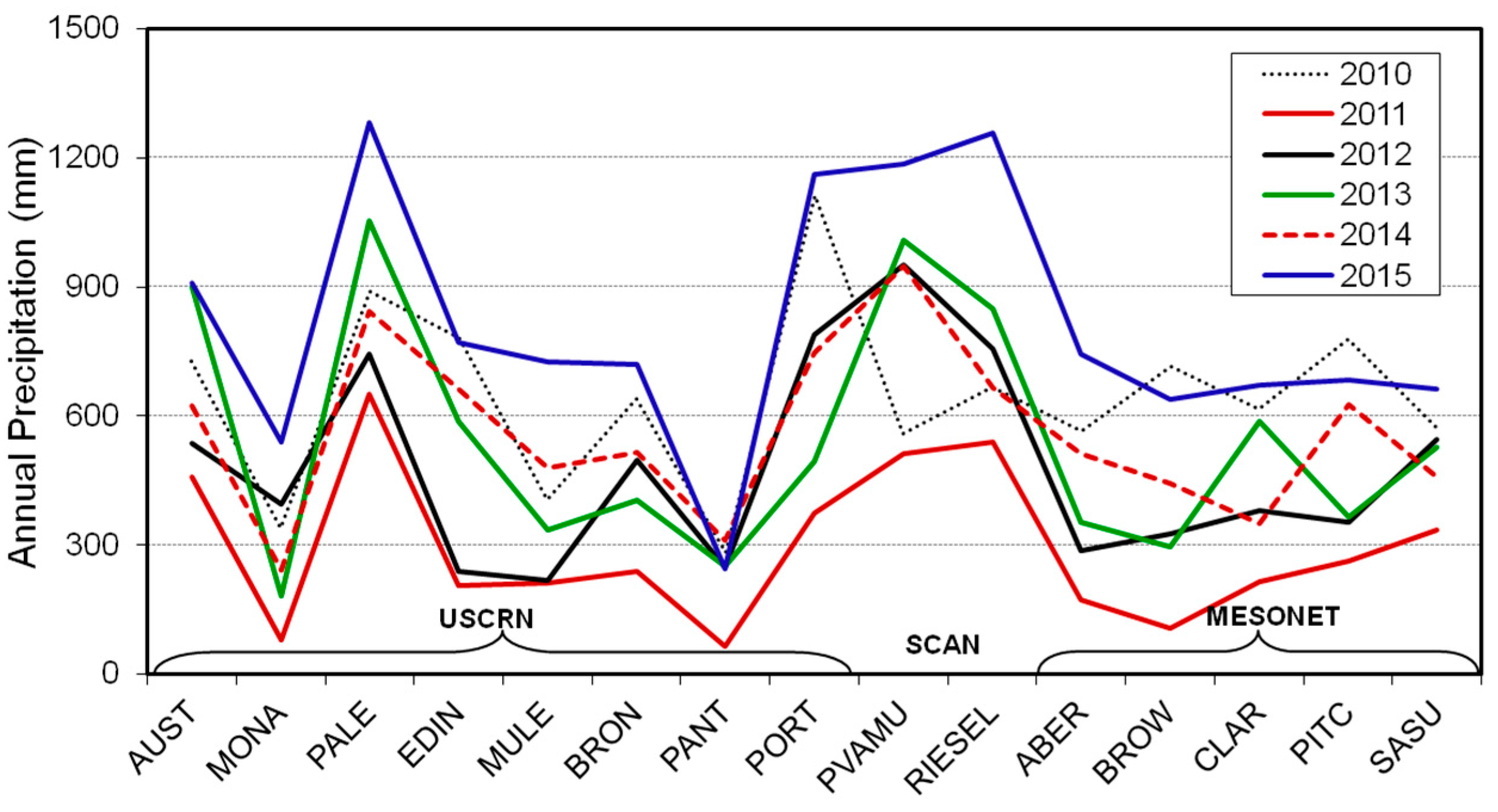
2.3. In Situ Measurements

This study used in situ SM data (at 5 cm) and precipitation measurements from the West Texas Mesonet [53], Soil Climate Analysis Network (SCAN) of the Natural Resources Conservation Service (NRCS) and the U.S. Climate Reference Network (USCRN) to compare it with satellite-generated SM data. The NRCS of the U.S. Department of Agriculture (USDA) operates the SCAN network, which consists of 129 observation stations in 39 states, with 14 in the state of Texas. The USCRN network consists of 114 stations in 48 states, with 8 in the state of Texas [54]. There were 5 Mesonet, 8 USCRN and 2 SCAN stations used in this study (Table 2). Table 2 provides a list of all in situ stations used, their coordinates, elevations and their surrounding land covers and soil types. Some of the Mesonet and SCAN stations were not included for analysis, as they had either no or only short periods of SM measurements or were clustered in only one or two climate zones and land covers. Data for SCAN stations are available at http://www.wcc.nrcs.usda.gov/scan/; data for West Texas Mesonet stations are available at http://www.mesonet.ttu.edu/; and data for USCRN stations are available at https://www.ncdc.noaa.gov/crn/. This study only used in situ soil moisture data measured at 5-cm soil depth.

2.4. Analysis Methods

This study evaluated satellite surface SM products by comparing the satellite diurnal measurements to each other and comparing them with in situ surface SM measurements from soil moisture monitoring networks which are considered as ground truths. Four satellite SM products were selected during the day overpasses either from ascending or descending passes. The selected SM products were from AMSR-E and AMSR2-Ascending (13.30 p.m.), SMOS-Ascending (6.00 a.m.) and SMAP-Descending (6.00 a.m.) passes.
First, dry and wet years were identified using precipitation data during the study period. Based on the precipitation data (2010–2015), 2011 received the least amount of rain (286 mm) and 2015 received the most rain (795 mm) in the state between 2010 and 2015 (Figure 3). On an average in 2011, the south, north, east and west regions of the state received 375, 216, 650 and 64 mm of precipitation, respectively, while in 2015 the same regions received 1163, 671, 1284 and 245 mm, respectively. For spatial distribution, evaluation was conducted by comparing spatial maps to each other using percentage of predicted wet and dry areas in the state.
Second, quality assurance and quality control (QA/QC) tests were performed, which led to the removal of several outliers and plateaus in the data. Third, spatial SM and LAI distribution maps were developed for the state of Texas for selected dry and wet days in a very dry year, 2011 and in a very wet year, 2015 during the study period (2010–2016) (Figure 4, Figure 5, Figure 6 and Figure 7).
Fourth, since the satellite SM measurements are not available for each day, a weekly moving average SM was calculated for each date by averaging a day’s SM with the six preceding days. Using weekly moving average soil moisture and in situ SM measurements, daily time series plots were developed focusing on overlapping periods. Also, since vegetation density has a significant impact on satellite SM quality, time series plots for LAI were also developed at each selected in situ station. When comparing the satellite SM with in situ measurements or with the temporal distributions of LAI, only those grid cells in which in situ measurement stations are located were considered for evaluation. Fifteen in situ stations were selected for detailed investigations. The selected in situ stations represent different major land covers and different climate zones in the state (Figure 1).
Fifth, the accuracy of each satellite product was evaluated using two statistical indicators: root mean square error (RMSE) and correlation coefficient (R). The R values were used to quantify the differences between various satellite soil moisture products and in situ soil moisture measurements. The RMSE values for in situ and satellite SM observations were calculated separately for each overlapping period: 2010–2011 (AMSR-E and SMOS), 2012–2016 (AMSR2 and SMOS), and 2015–2016 (SMAP, AMSR2 and SMOS). The unbiased RMSE has been used recently for the assessment of soil moisture products [19,33,55] where the seasonal mean was considered. In this study, the standard RMSE was used, as we are intercomparing different products covering different time periods and different durations, which may introduce discrepancies in the effect of the climatology on the soil moisture assessment.
Overall, the comparison of satellite SM data to each other as well as to in situ measurements during the overlapping period, helped to evaluate the performance of satellite soil moisture products not only using in situ point measurements alone but in combination with the satellite measurements.

3. Results

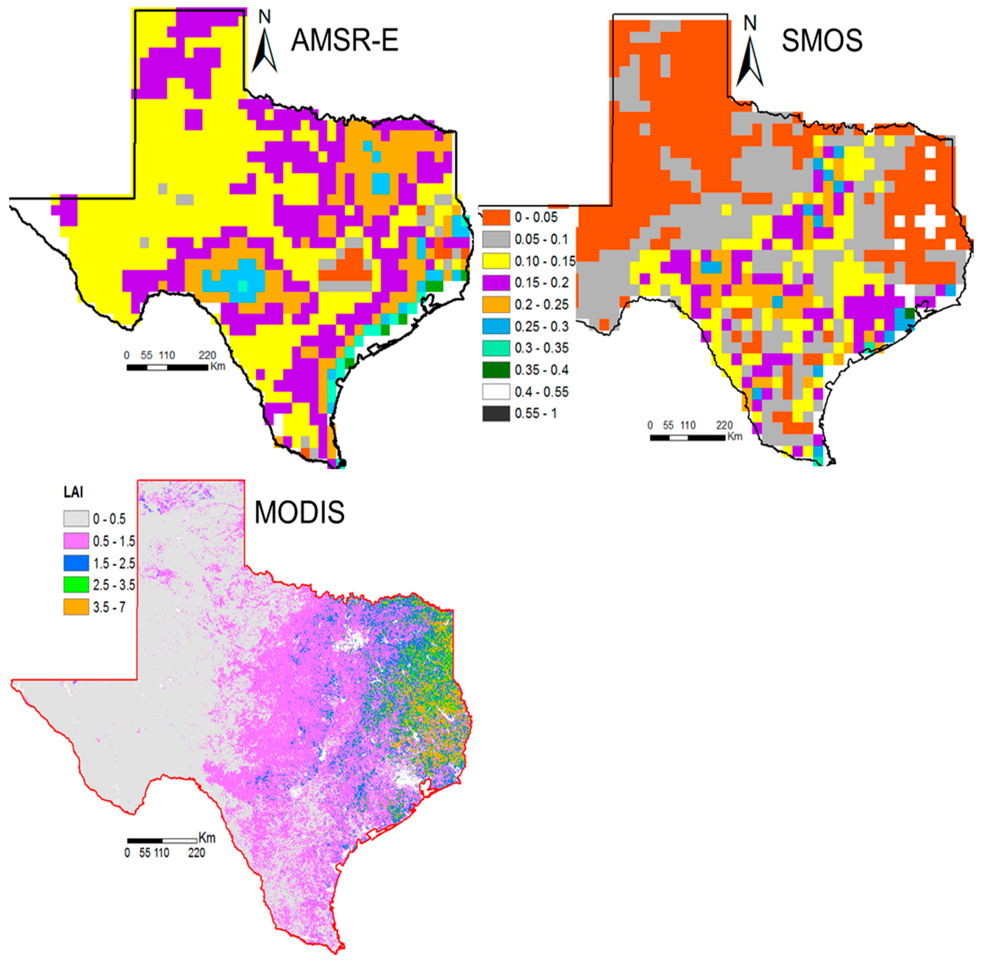
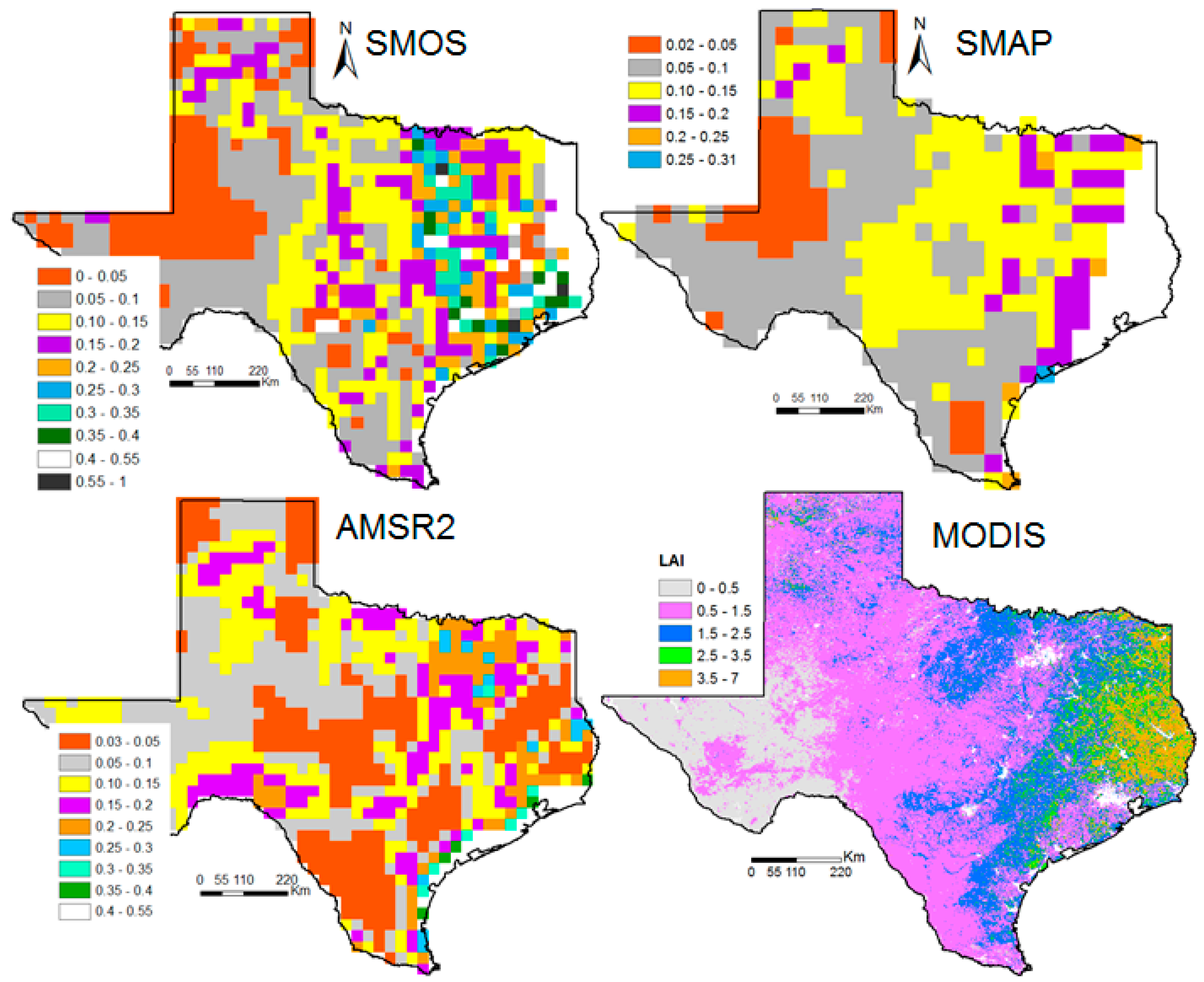
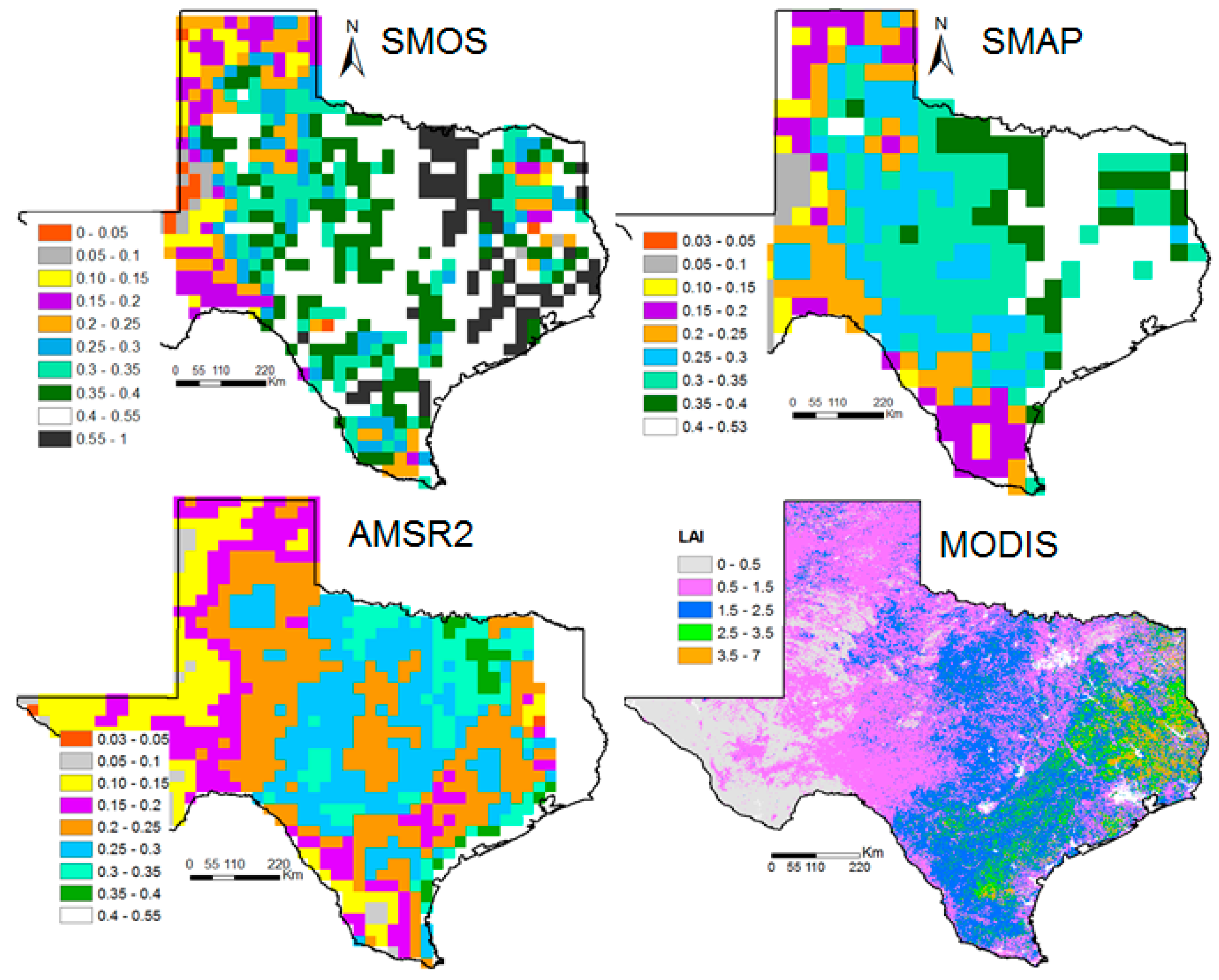
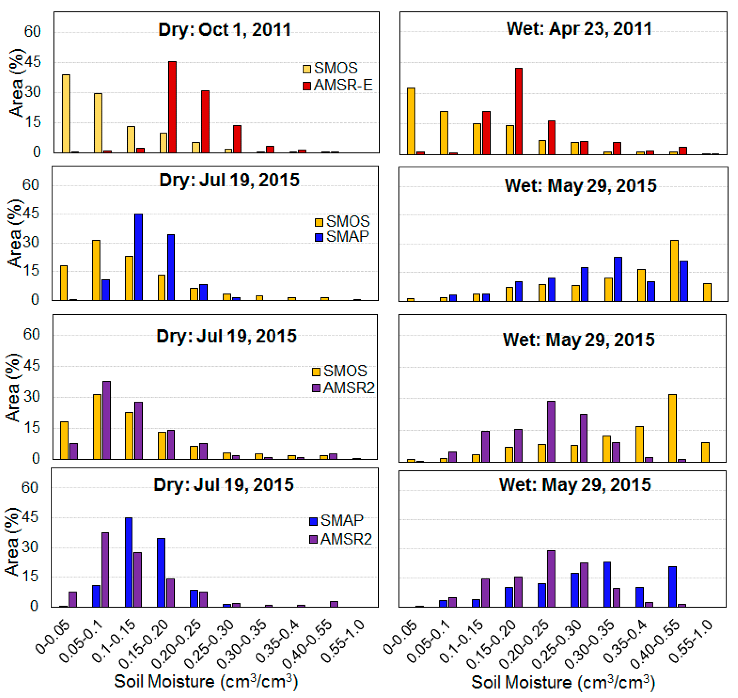
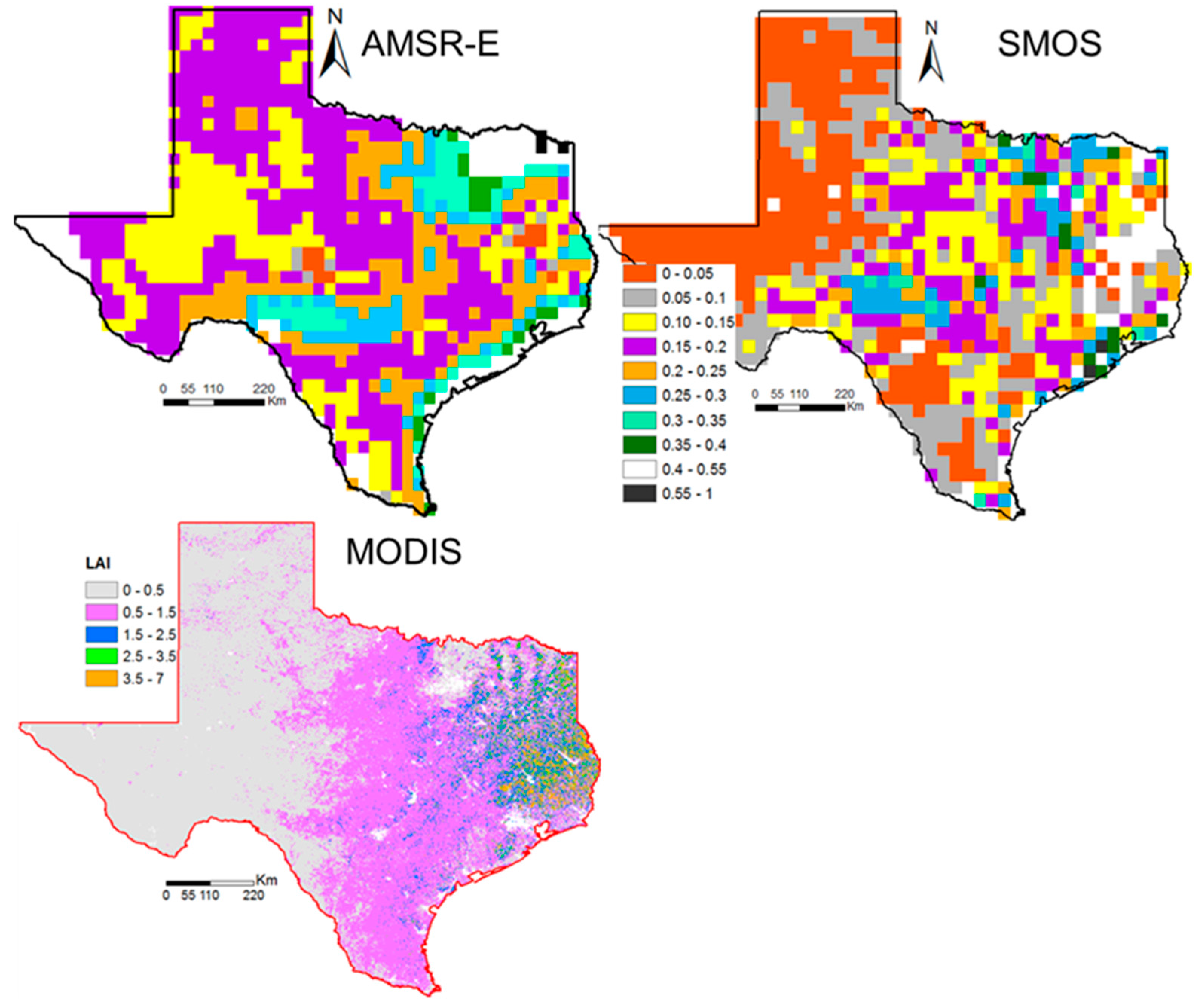
3.1. Evaluation Using Spatial Variation

Figure 4, Figure 5, Figure 6 and Figure 7 show the spatial distribution of SM from AMSR-E, AMSR2, SMOS and SMAP satellites and LAI distribution from MODIS satellite for selected dry and wet days in 2011 and 2015. The years 2011 and 2015 were selected as driest and wettest years, respectively, to compare SM distribution measured by four different satellites during the study period. This study focused on satellite SM measurements during an overlapping period, as AMSR-E had overlapped with SMOS (2010–2011), SMOS has been overlapping with SMAP (2015–present) and AMSR2 has been overlapping with SMOS (2012–present) and SMAP (2015–present).
AMSR-E and SMOS surface SM products for 1 October 2011, which was the driest day in the year, were compared (Figure 4). AMSR-E SM values (in cm3/cm3) ranged from 0 to 0.47, whereas SMOS SM values ranged from 0 to 1, which showed SMOS upper range SM observations were higher than AMSR-E. Comparatively, AMSR-E identified the drier west of Texas as wetter than the SMOS observations in 2011. AMSR-E and SMOS identified 0.4% and 39% of the area of Texas, respectively, as having SM between 0 and 0.05 cm3/cm3 for that day. On the other hand, AMSR-E and SMOS identified 45% and 13% of the area of Texas, respectively, as having SM between 0.1 and 0.15 cm3/cm3 (Figure 8).
Figure 5 compares AMSR-E and SMOS surface SM products for 22 April 2011. AMSR-E SM ranged from 0.05 to 0.59 cm3/cm3, and SMOS SM values were still from 0 to 1 cm3/cm3, which showed SMOS observations were wetter than those for AMSR-E based on the maximum SM values. However, AMSR-E and SMOS identified 42% and 14% of the area of Texas, respectively, as having SM values between 0.15 and 0.20 cm3/cm3. Yet, AMSR-E and SMOS identified 17% and 7% of the area of Texas, respectively, as having SM values between 0.2 and 0.25 cm3/cm3 (Figure 8). The LAI distribution maps were included to evaluate satellite performance when the density of vegetation had any impact on quality of SM. In the drought year of 2011, there was no significant change in LAI (vegetation density) in a wet month (April) and a dry month (October). Therefore, in a drought year, vegetation pattern had no significant role in controlling satellite SM quality because LAI values remained low for most of the state in both months. The analysis showed 87% (October) and 91% (April) of the state’s area had LAI values between 0 and 1.5 whereas only 3% (October) and 1.9% (April) of the state’s area had LAI values between 3.5 and 7.
Figure 6 compares SMOS, AMSR2 and SMAP surface SM measurements on 19 July 2015, which was the driest day in 2015. The SMOS SM values ranged from 0 to 1 cm3/cm3 and AMSR2 SM values ranged from 0.03 to 0.55 cm3/cm3, whereas SMAP SM values ranged from 0.02 to 0.31 cm3/cm3, which showed SMOS observations were wetter than AMSR2 and SMAP observations based on the measured maximum SM values. However, in comparison, all three satellites had good agreement on SM distribution over the west of Texas on the dry day of the wet year 2015. On the other hand, SMAP SM measurements were comparatively lower than SMOS and AMSR2 measurements for the east of Texas. AMSR2, SMOS and SMAP identified 8%, 18% and 0.3% of the state’s area, respectively, as having SM less than 0.05 cm3/cm3, while these same three systems identified 28%, 23% and 45% of the state’s area, respectively, as having SM values between 0.1 and 0.15 cm3/cm3 (Figure 8).
Figure 7 compares SMOS, AMSR2 and SMAP surface SM measurements on 29 May 2015, which was the wettest day in 2015. The SMOS and AMSR2 SM values were still from 0 to 1 cm3/cm3, and 0.03 to 0.55 cm3/cm3, respectively, but the range of SMAP SM values increased from 0.02 to 0.31 cm3/cm3 to 0.02 to 0.53 cm3/cm3, which showed, qualitatively SMAP observed higher SM for wetter days. However, maximum SM values from SMOS satellite were still higher than those for AMSR2 and SMAP. In comparison, all three satellites had good agreement on SM spatial distribution over the drier west of Texas on the wet day of the wet year 2015. However, only AMSR2 and SMAP had good agreement over the mid and east of Texas on a very wet day. On the other hand, SMOS SM measurements showed mid-Texas was wetter whereas both AMSR2 and SMAP SM measurements showed mid-Texas was comparatively drier. AMSR2, SMOS and SMAP identified only 0.4%, 1.2% and 0% of the state’s area, respectively, as having SM less than 0.05 cm3/cm3, and 23%, 8% and 17% of the area, respectively, as having SM between 0.25 and 0.30 cm3/cm3. The SMOS identified that 32% of Texas had SM between 0.4 and 0.55, and SMAP identified only 21% of Texas had SM between 0.4 and 0.55 cm3/cm3. However, AMSR2 identified only 1.3% of Texas had SM values between 0.4 and 0.55 (Figure 8).
In comparison, since there was only about two months in the time difference between selected dry and wet days, no significant change in LAI distribution was observed. For example, the analysis showed 62% (May) and 72% (July) of area in the state had LAI values between 0 and 1.5, and 34% (May) and 25% (July) of area had LAI values between 1.5 and 3.5, whereas only 3.2% and 5.2% of area, respectively, in May and July had LAI values between 3.5 and 7. Therefore, since most of the state is covered with vegetation with low density, LAI distribution or vegetation density had no significant impact on the quality of SM measurements by various satellites in the state.

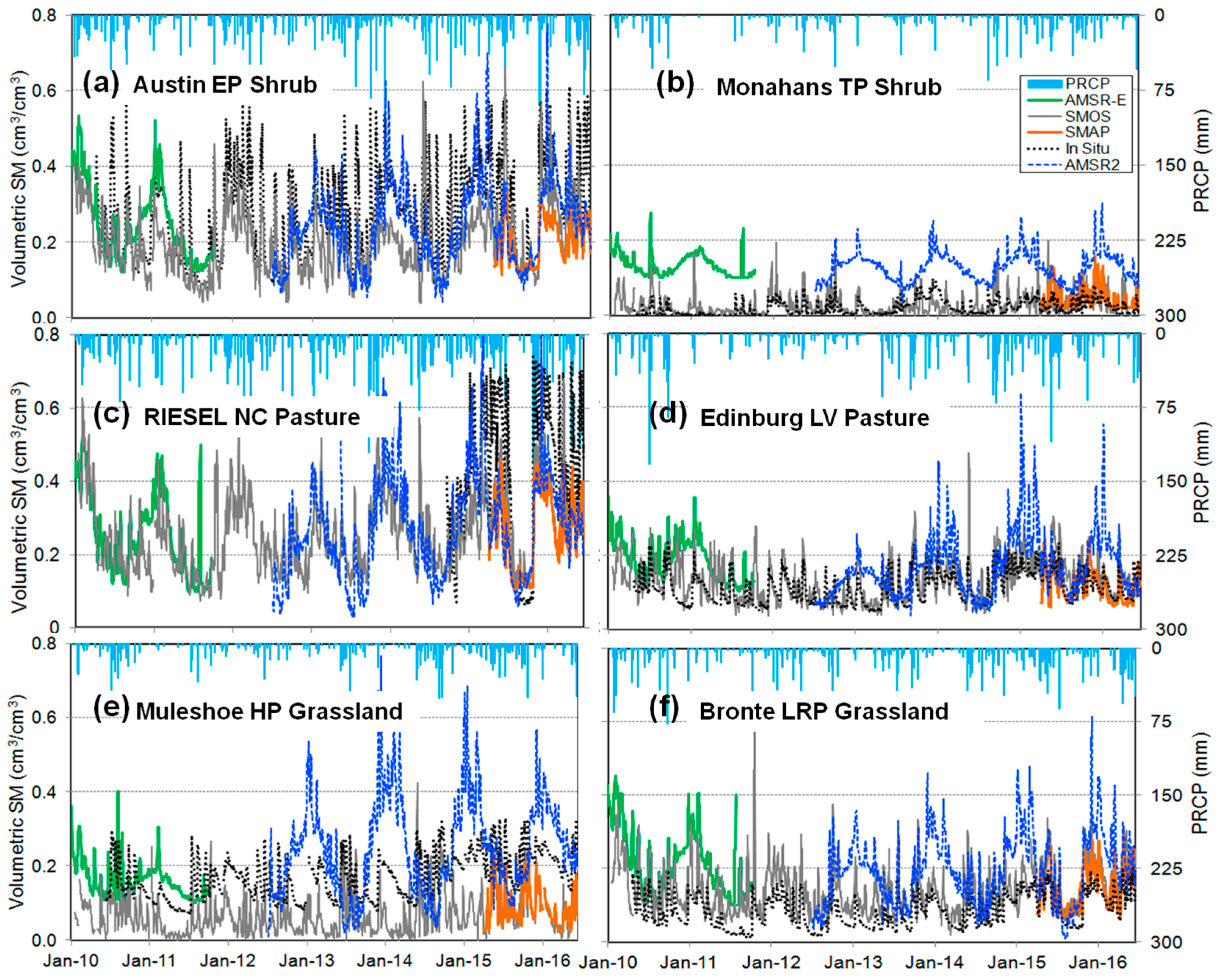
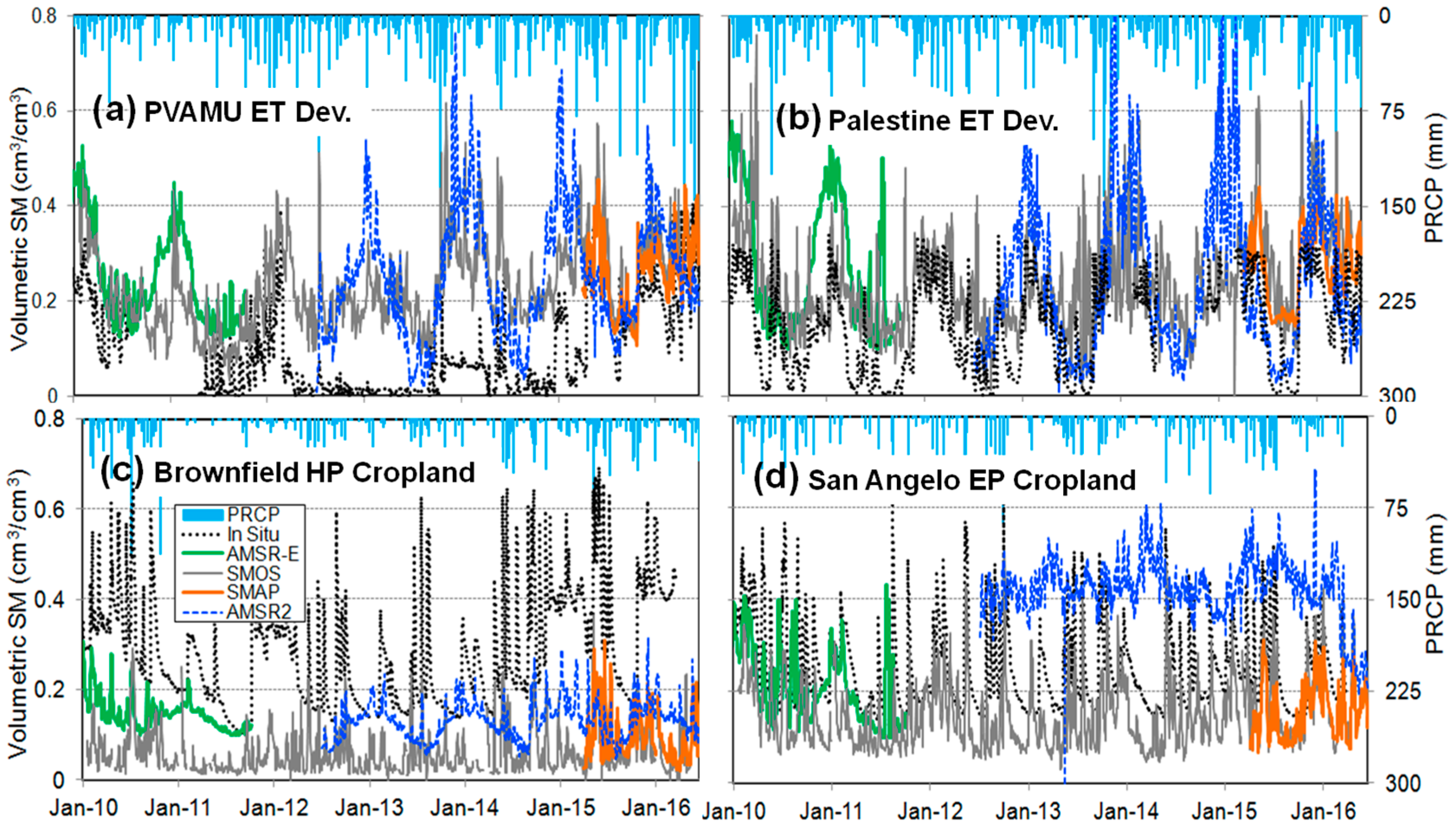
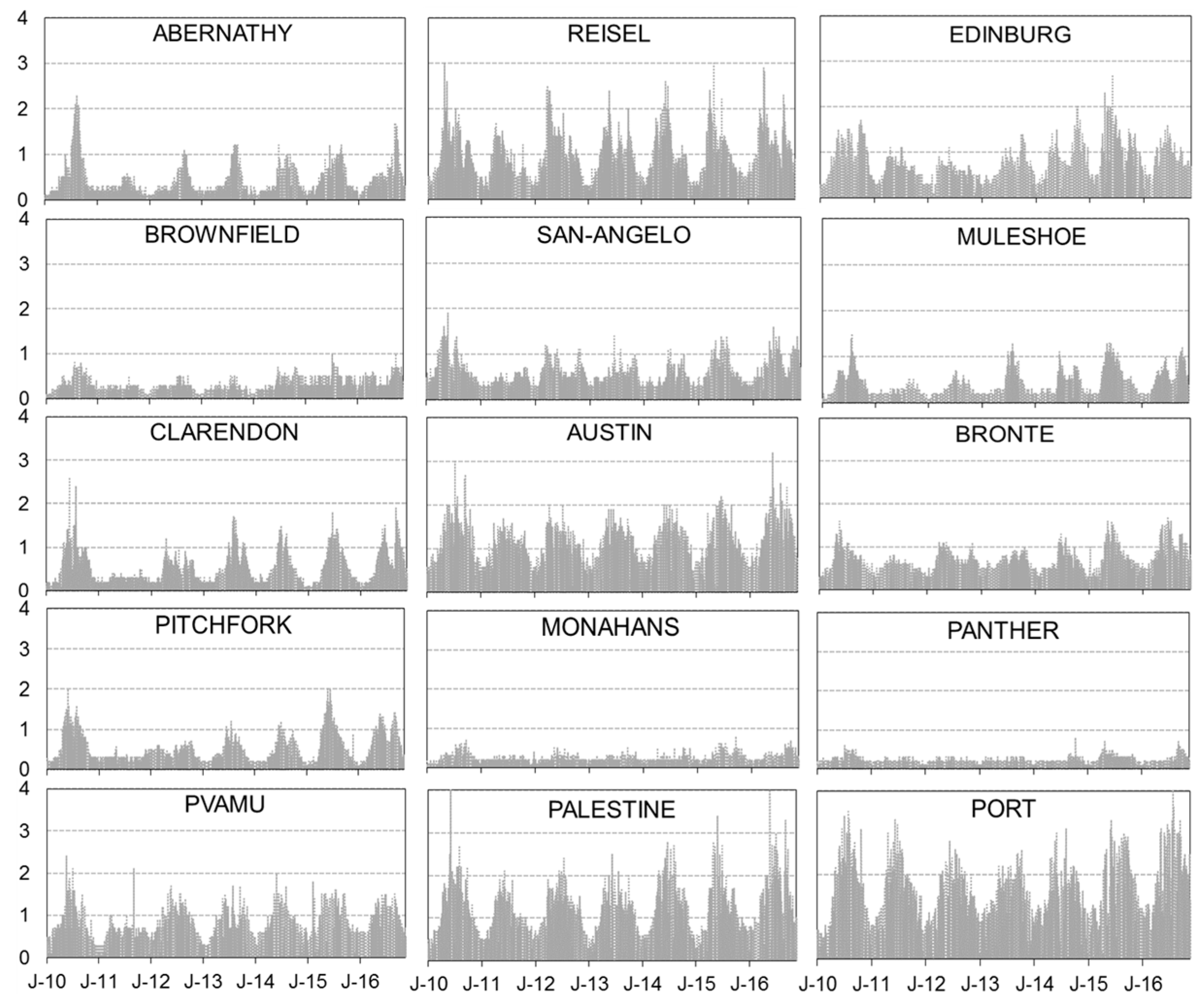
3.2. Evaluation Using Temporal Variation

Figure 9 shows a time series of the daily surface SM observations from four different satellites and daily in situ precipitation and surface SM (0–5 cm) at 10 different locations in the state of Texas from 2010 to 2016. For direct comparison and evaluation, precipitation and SM measurements were presented together on a single graph for the respective in situ stations and the selected pixel level of satellite footprint scale. When selecting the in situ SM stations and satellite grids, it was taken into account that each land cover should represent two different climate zones. Altogether, SM and precipitation distributions were presented at eight major climate zones for five major land covers (Figure 9 and Table 3 and Table 4). The SM distributions for shrub land cover were compared at Austin (EP climate zone (CZ)) and Monahans (TP CZ), pasture land at Riesel (NC CZ) and Edinburg (LV CZ) and grassland at Muleshoe (HP CZ) and Bronte (LRP CZ). Similarly, SM distributions for the development regions at PVAMU (ET CZ) and Palestine (ET CZ) and for the croplands at Brownfield (HP CZ) and San Angelo (EP CZ) locations were also compared and evaluated.
In comparison to in situ SM observations, AMSR-E always under-predicted over cropland and development land covers despite their locations at ET, HP or EP climate zones. However, AMSR-E had comparatively better performance over shrub and grassland land covers with loamy sand and worse performance over forest land with sandy soil (Table 3). The performance of AMSR-E was not consistent over the same land cover at two different or same climate zones and in the same climate zone over two different or same land covers. For example, within ET climate zone, correlation coefficient (R) between AMSR-E and in situ SM measurements at PVAMU and Palestine developed regions were respectively, 0.61 and 0.65. Similarly, for grassland, correlation coefficients at Abernathy (HP) and Bronte (LRP) locations were 0.35 and 0.63, respectively (Table 3).
The AMSR-E SM product was only overlapped with SMOS SM product from 2010 to 2011. The R values between AMSR-E and SMOS SM measurements were not consistent and they varied from 0.03 (lowest) at TP climate zone over shrub land and open developed region to 0.66 (highest) at ET climate zone over pasture land cover (Table 4).
As shown in Figure 9 and Figure 10, the difference between low and high SM observations of SMOS was higher than AMSR-E and SMAP SM observations and lower than the AMSR2 SM observation. In comparison to in situ SM observation, SMOS under-predicted over cropland at both HP and EP climate zones whereas for grassland, SMOS over-predicted at LRP climate zone and under-predicted at HP climate zone. However, for developed region, SMOS prediction was higher than in situ measurements. On the other hand, SMOS had the comparatively better performance for the shrub (Austin) and the pasture (Riesel and Edinburg) land covers at EP, NC and LV climate zones (R = 0.71, 0.78 and 0.63, respectively, Table 3). The performance of SMOS was consistent over the grassland, cropland, developed and pasture land covers at two different or same climate zones, but it was inconsistent over the shrub land cover. For example, under TP climate zone, R values between SMOS and in situ SM measurements at Monahans and Panther locations with shrub land cover were, respectively, 0.26 and 0.56. Similarly, for shrub land cover, R values at Clarendon (LRP) and Austin (EP) were 0.24 and 0.71, respectively (Table 3).
The SMOS SM product has been overlapping with all three satellite SM products used in this study; AMSR-E (2010–October-2011), AMSR2 (July-2012–present) and SMAP (March-2015–present). The R values between SMOS and AMSR2 SM measurements were not consistent and ranged from 0.1 (lowest) at EP climate zone over cropland to 0.59 (highest) at NC climate zone over pasture land cover (Table 4). On the other hand, the correlation between SMOS and SMAP data was very high (R = 0.66–0.91) compared to inter-correlations among any other satellites used in this study.
The range between low and high of AMSR2 SM measurements was also higher than AMSR-E, SMOS and SMAP SM observations. Compared to in situ SM observation, AMSR2 had over-predicted over grassland at both HP and LRP climate zones, whereas, for the cropland, AMSR2 had over-predicted at EP climate zone and under-predicted at HP climate zone. However, for the developed region, the AMSR2 prediction was higher than in situ measurements. On the other hand, AMSR2 had comparatively better performance over the shrub (Austin) and the pasture (Riesel) land covers at EP and NC climate zones (R = 0.62, 0.60 and 0.63, respectively, Table 3). Like AMSR-E, the performance of AMSR2 was also not consistent over the same land cover at two different or same climate zones and at same climate zone over two different or same land covers. For example, within ET climate zone, R values between AMSR2 and in situ SM measurements at PVAMU and Palestine developed regions were respectively, 0.14 and 0.53. Similarly, for shrub land, R values at Clarendon (LRP) and Austin (EP) were 0.57 and 0.62, respectively, whereas at Monahans (TP) and Panther (TP), R values were 0.26 and 0.24, respectively (Table 3). Interestingly, unlike AMSR-E, the performance of AMSR2 over grassland was consistent at selected four locations and two climate zones (HP, LRP) because the R values ranged from 0.39 to 0.60.
The AMSR2 SM product has been overlapping with SMOS and SMAP SM products; SMOS (July-2012–present) and SMAP (March-2015–present). However, the R values between SMAP and AMSR2 SM measurements were not consistent throughout the state of Texas, as they ranged from 0.10 (lowest) at EP climate zone over cropland to 0.80 (highest) at NC climate zone over pasture land cover; R values between AMSR2 and SMAP were high (R = 0.46–0.80) at a majority of selected locations/land covers (Table 4).
The SMAP SM measurements were available relatively for a shorter period (~1.5 years), only from 2015 to 2016. It is worth noting that both 2015 and 2016 years were considered wet during the study period. Compared to in situ SM observations, SMAP had predicted reasonably well almost at all of the climate zones and over major land covers except over cropland at Brownfield (HP) and shrub land at Monahans (TP). The R values were 0.45 and 0.37, respectively, at Brownfield and Monahans locations. The R values for the rest of the selected locations ranged from 0.60 to 0.92 (Table 3). Although the R values showed the SMAP performed well over all of the selected land covers and climate zones, quantitatively the SMAP SM observations were not consistent throughout the state. For example, the SMAP had predicted lower SM values than in situ measurements over grassland at Muleshoe (HP), shrub land at Austin (EP), cropland at Brownfield (HP) and slightly higher values at Monahans (TP). The SMAP SM product has been overlapping with SMOS and AMSR2 SM products, and R values between SMAP and AMSR2 and SMAP and SMOS SM measurements are discussed earlier.
Table 5 presents root mean square error (RMSE) values among in situ and satellite soil moisture observations for the overlapping periods. Analysis showed RMSE for AMSR-E and SMOS with respect to in situ observations ranged from 0.08 to 0.37 and 0.04 to 0.28 cm3/cm3, respectively (2010–2011). The RMSE for AMSR2 and SMOS with respect to in situ observations ranged from 0.09 to 0.41 and 0.04 to 0.32 cm3/cm3, respectively (2012–2016), whereas RMSE for SMAP, AMSR2 and SMOS ranged from 0.02 to 0.35, 0.08 to 0.47 and 0.03 to 0.32 cm3/cm3 (2015–2016), respectively. However, on an average, for all 15 in situ stations, these values were 0.09 (AMSR-E), 0.16 (AMSR2), 0.14 (SMOS) and 0.13 (SMAP), respectively.
In comparison, average RMSE value for AMSR-E was one of the lowest among all satellites, but it had a larger RMSE range (0.08–0.37 cm3/cm3). Moreover, a 0.13 cm3/cm3 RMSE value for the range of 0–0.59 cm3/cm3 SM was a 44% deviation from its mean. On the other hand, AMSR2, SMOS and SMAP had larger SM observation ranges: 0.01–0.99, 0.001–0.99 and 0.02–0.5 cm3/cm3, respectively, which had 28%, 32% and 49% deviations from their means, respectively. Although the RMSE values also rely on other factors such as the duration of observation, the calculated average RMSE values of all four satellite SM products were very close to each other (Table 5).
Figure 8 presents time series plots (4-day MODIS LAI composite) of LAI at selected fifteen in situ stations at MODIS grid scale. Results showed a majority of selected locations had low LAI values (≤2) during the study period. On the other hand, only a few locations (e.g., Riesel, Austin, Palestine and Port) had LAI values larger than 2 during the study period. This study used LAI time series patterns to study the impact of vegetation density on satellite SM quality.

4. Discussion

This study evaluated the performance of four different satellite surface SM products generated for the state of Texas. One of the important aspects of this evaluation was that three of four used satellite SM products have the same footprint scale (25 km), except the SMAP SM product, which has a 36-km footprint scale which was re-sampled to 25-km scale. In Texas, whether it is a dry or wet year, the west part of the state always remains drier compared to the east. Performances of all four satellites were poorer in the west of the state and better in the east, despite low vegetation density in the west and high vegetation density in the east.
Researchers have agreed there is a strong correlation between satellite SM quality and vegetation density, as the quality of SM data decreases with the increase of vegetation density (e.g., [16,48,56,57]). There was an agreement between the vegetation density and satellite performance to measure surface SM over different land covers with low or high density in the east region (humid). For example, this was so at four locations (Austin 1.1–3.2 (Average to Maximum LAI values), Riesel 1.0–3.0, Palestine 1.2–5.1 and Port 1.5–4.1) with higher LAI values, though satellite performance was poor. However, in comparison, the performance of SMAP was better than SMOS, followed by AMSR2 and AMSR-E, despite higher vegetation density in the eastern part of Texas. However, the performance of all four satellites was poor over the forest land cover (Port, LAI 1.5–4.1), which had comparatively higher vegetation density (Figure 11). On the other hand, regardless of vegetation density (low or high), performances of satellites were poor in the west of Texas, which showed that it was not only the vegetation density which could impact a satellite’s performance; other factors such as climate may have significant impacts on their performances. This is in line with the findings of Champagne et al. [48], as SMOS SM products were also impacted by local surface temperature, vegetation water content, surface roughness and/or topography.
During the drought year 2011, AMSR-E and SMOS SM values ranged from 0–0.47 cm3/cm3 and 0–1 cm3/cm3, respectively, on a selected dry day, whereas on a wet day SM values ranged from 0–0.59 cm3/cm3 and 0–1 cm3/cm3, respectively. On the other hand, AMSR-E predicted more area wetter than SMOS both on dry and wet days. Analysis showed a very small percentage of area (0% on a dry day and 0.2% on a wet day) predicted by SMOS had SM values more than the upper range of AMSR-E (0.59). These findings are in line with the findings of other researchers. For example, SMOS tends to underestimate soil moisture in arid areas (e.g., [58,59]). During 2015, a wet year, lower and upper limits of SMOS, AMSR2 and SMAP SM values were different. For example, SMOS, AMSR2 and SMAP SM values ranged from 0–1, 0.05–0.55 and 0.02–0.31 cm3/cm3, respectively, on selected dry day and 0–1, 0.03–0.55 and 0.02–0.53 cm3/cm3, respectively, on selected wet day in 2015. Analysis showed all three satellites performed reasonably well in identifying drier and wetter regions in the state, but SMAP performance was best among all.
The satellite’s performance over the same land cover at two different climate zones or within the same climate zones at two different locations was not consistent. However, the performance of SMAP was best among all, which could be due to a shorter period of observations and/or SMAP observations used in this study, which were only from two wet years. The comparison of satellite SM over the same land cover, but at different climate zones, presented an overview of the impact of heterogeneities such as climate, vegetation and topography on satellite SM retrievals and methods to estimate SM in the state of Texas. In addition, inconsistencies among satellite performances were also because of differences in their over-passing times, band or frequency of sensors, retrieval algorithms used and radio frequency interference (RFI), which was in line findings by Jackson et al. [59] that there was significant impact of over-passing time and frequency/wavelength on the performance of retrieval algorithms, which has direct impact on the satellite performance. To narrow the impact of some of those factors, this study selected AMSR-E and AMSR2 which had same passing time and frequency (ascending at 1.30 p.m. local time, X-band (10.65 GHz.)). Similarly, this study also selected SMAP (descending at 6 a.m. local time, L-band (1.41 GHz.)) and SMOS (ascending at 6 a.m. local time, L-band (1.4 GHz.) which had the same passing time and band/frequency. However, the performances of AMSR-E and AMSR2 or SMOS and SMAP were not consistent over the selected land cover and climate zones, which could indicate there are still issues needed to be addressed in the study region or other regions with comparable climate, land cover and topographic heterogeneities.
Since this study was focused on evaluating satellite SM during their overlapping periods, in situ point measurements at various locations in the state were used to understand how close each satellite surface SM measurements align with the in situ SM measurements. Despite the considerable heterogeneity within the satellite footprint scale and throughout the state, each satellite performed reasonably well, especially during the wet year and humid region in the state of Texas.

5. Conclusions

Soil moisture is a key parameter of the hydrological and meteorological conditions of a given location. Several remote sensing satellites have been launched to monitor SM at different temporal and spatial scales and have different levels of uncertainties in their measurements. Evaluation of satellite SM products is important at regional to global scales, particularly over the different climate zones and land covers. This study evaluated four satellite SM products across the state of Texas using in situ SM measurements as well as taking advantage of the satellites’ overlapping durations during the study period.
Analysis showed the satellite SM products captured the seasonal variations, however, they were not consistent in capturing the temporal variations. The AMSR-E underestimated SM whereas AMSR2 overestimated SM at most of the locations and times. On the other hand, SMOS underestimated SM during the dry season and it performed better during the wet season, which is in line with the findings of Leroux et al. [60] over four watersheds in the US. The SMAP performed best during the dry and wet season of the wet years, however, SMAP needs to be tested in drought years because both 2015 and 2016 were considered wet years when SMAP SM products were evaluated.
All of the satellites had comparatively poor performance in SM estimation over dry regions and during the dry period, though the performance of SMAP was better among all of the used satellites over the state of Texas. The major reasons for poor performances could be the significant heterogeneity such as climate, topography, vegetation/land cover present in the study region, which supports the findings of Njoku and Entekhabi [25], that the impact of spatial heterogeneity of vegetation cover and subsurface soil characteristics at footprint scale limit the performance of satellite SM retrieval at large scale. However, it is noted that it is not only the vegetation density which can impact a satellite’s performance in capturing soil moisture variability; other factors such as climate, soil characteristics and topography may have a significant impact on their performance.
Further studies are needed to investigate the effects of heterogeneity in land cover and climate on satellite SM observations, with more combination of in situ observations with hydrologic models that simulate soil moisture. In addition, since the performance of satellites was not consistent in this study region, it is, therefore, important to investigate SM data from ascending and descending passes to confirm which pass of a particular satellite has better performance. Other researchers (e.g., [36,61,62,63]) have pointed out that both day- and night-time retrievals have some advantages and disadvantages, as diurnal variations might have a negative impact on the accuracy during the day and isothermal conditions at night might reduce the errors caused by surface temperature variations.
Overall, this study analyzed inconsistencies among four different satellite SM products over the state of Texas and found challenges to have a consistent satellite SM product in a climate and land cover over a heterogeneous region, which suggests the need for additional investigations, including in algorithms used to generate satellite soil moisture data.

Acknowledgments

This work has been partially funded by the Evans-Allen project of the National Institute of Food and Agriculture of the United States Department of Agriculture (USDA). We thank USDA Natural Resources Conservation Service, The West Texas Mesonet and The U.S. Climate Reference Network for providing in situ soil moisture data. We thank Richard McWhorter for his time to edit this paper. We also thank the editor and two anonymous reviewers for their comments and suggestions, which helped us to improve the quality of this manuscript.

Author Contributions

Ram Ray, Ali Fares and Marouane Temimi developed approaches and methods for this manuscript; Ram Ray outlined the manuscript; Yiping He and Ram Ray downloaded, developed and analyzed the remotely-sensed data; Ali Fares and Marouane Temimi contributed in methodology and discussion of this manuscript; Ram Ray wrote the paper.

Conflicts of Interest

The authors declare no conflict of interest.

References

  1. Seneviratne, S.I.; Corti, T.; Davin, E.L.; Hirschi, M.; Jaeger, E.B.; Lehner, I.; Orlowsky, B.; Teuling, A.J. Investigating soil moisture-climate interactions in a changing climate: A review. Earth-Sci. Rev. 2010, 99, 125–161. [Google Scholar] [CrossRef]
  2. Al Bitar, A.; Leroux, D.; Kerr, Y.H.; Merlin, O.; Richaume, P.; Sahoo, A.; Wood, E.F. Evaluation of SMOS Soil Moisture Products Over Continental US Using the SCAN/SNOTEL Network. IEEE Trans. Geosci. Remote Sens. 2012, 50, 1572–1586. [Google Scholar] [CrossRef]
  3. Griesfeller, A.; Lahoz, W.A.; de Jeu, R.A.M.; Dorigo, W.; Haugen, L.E.; Svendby, T.M.; Wagner, W. Evaluation of satellite soil moisture products over Norway using ground-based observations. Int. J. Appl. Earth Obs. Geoinf. 2016, 45, 155–164. [Google Scholar] [CrossRef]
  4. Xiao, Z.; Jiang, L.; Zhu, Z.; Wang, J.; Du, J. Spatially and Temporally Complete Satellite Soil Moisture Data Based on a Data Assimilation Method. Remote Sens. 2016, 8. [Google Scholar] [CrossRef]
  5. Huszar, T.; Mika, J.; Loczy, D.; Molnar, K.; Kertesz, A. Climate change and soil moisture: A case study. Phys. Chem. Earth Part A Solid Earth Geod. 1999, 24, 905–912. [Google Scholar] [CrossRef]
  6. Li, H.B.; Robock, A.; Wild, M. Evaluation of Intergovernmental Panel on Climate Change Fourth Assessment soil moisture simulations for the second half of the twentieth century. J. Geophys. Res.-Atmos. 2007, 112. [Google Scholar] [CrossRef]
  7. Collow, T.W.; Robock, A.; Basara, J.B.; Illston, B.G. Evaluation of SMOS retrievals of soil moisture over the central United States with currently available in-situ observations. J. Geophys. Res.-Atmos. 2012, 117, D09113. [Google Scholar] [CrossRef]
  8. Dorigo, W.A.; Wagner, W.; Hohensinn, R.; Hahn, S.; Paulik, C.; Xaver, A.; Gruber, A.; Drusch, M.; Mecklenburg, S.; van Oevelen, P.; et al. The International Soil Moisture Network: A data hosting facility for global in-situ soil moisture measurements. Hydrol. Earth Syst. Sci. 2011, 15, 1675–1698. [Google Scholar] [CrossRef]
  9. Wagner, W.; Dorigo, W.; de Jeu, R.; Fernandez, D.; Benveniste, J.; Haas, E.; Martin, E. Fusion of active and passive microwave observations to create an essential climate variable data record on soil moisture. ISPRS Ann. Photogramm. Remote Sens. Spat. Inf. Sci. 2012, 315–321. [Google Scholar] [CrossRef]
  10. Henderson-Sellers, A. Soil moisture: A critical focus for global change studies. Globa. Planet. Chang. 1996, 13, 3–9. [Google Scholar] [CrossRef]
  11. Korres, W.; Reichenau, T.G.; Schneider, K. Patterns and scaling properties of surface soil moisture in an agricultural landscape: An ecohydrological modeling study. J. Hydrol. 2013, 498, 89–102. [Google Scholar] [CrossRef]
  12. Schoonover, J.E.; Crim, F. An introduction to soil concepts and the role of soil in watershed management. J. Contemp. Water Resear. Educ. 2015, 154, 21–47. [Google Scholar] [CrossRef]
  13. Fares, A.; Temimi, M.; Morgan, K.T.; Kelleners, T.J. In-situ and remote soil moisture sensing technologies for vadose zone hydrology. Vadose Zone J. 2013, 12. [Google Scholar] [CrossRef]
  14. Temimi, M.; Lakhankar, T.; Zhan, X.; Cosh, M.H.; Krakauer, N.; Fares, A.; Kelly, V.; Khanbilvardi, R.; Kumassi, L. Soil moisture retrieval using ground-based L-band passive microwave observations in Northeastern USA. Vadose Zone J. 2014, 13. [Google Scholar] [CrossRef]
  15. GCOS. Systematic observation requirements for satellite based data products for climate. GCOS 2011, 154, 1–127. [Google Scholar]
  16. Brocca, L.; Hasenauer, S.; Lacava, T.; Melone, F.; Moramarco, T.; Wagner, W.; Dorigo, W.; Matgen, P.; Martinez-Fernandez, J.; Llorens, P.; et al. Soil moisture estimation through ASCAT and AMSR-E sensors: An intercomparison and validation study across Europe. Remote Sens. Environ. 2011, 115, 3390–3408. [Google Scholar] [CrossRef]
  17. Notarnicola, C.; Caporaso, L.; Giuseppe, F.D.; Temimi, M.; Ventura, B.; Zebisch, M. Inferring soil moisture variability in the Mediterrean Sea area using infrared and passive microwave observations. Can. J. Remote Sens. 2012, 38, 46–59. [Google Scholar] [CrossRef]
  18. Nicolai-Shaw, N.; Hirschi, M.; Mittelbach, H.; Seneviratne, S.I. Spatial representativeness of soil moisture using in-situ, remote sensing, and land reanalysis data. J. Geophys. Res.-Atmos. 2015, 120, 9955–9964. [Google Scholar] [CrossRef]
  19. Kumar, S.V.; Peters-Lidard, C.D.; Mocko, D.; Reichle, R.; Liu, Y.; Arsenault, K.R.; Xia, Y.; Michael, E.K.; George, R.; Livneh, B.; et al. Assimilation of remotely sensed soil moisture and snow depth retrievals for drought estimation. J. Hydrometeorol. 2014, 15, 2446–2469. [Google Scholar] [CrossRef]
  20. Lakhankar, T. Estimation of Soil Moisture Using Microwave Remote Sensing Data. Ph.D. Thesis, The City University of New York, New York, NY, USA, 2006. [Google Scholar]
  21. Dorigo, W.; de Jeu, R.; Chung, D.; Parinussa, R.; Liu, Y.; Wagner, W.; Fernandez-Prieto, D. Evaluating global trends (1988–2010) in harmonized multi-satellite surface soil moisture. Geophys. Res. Lett. 2012, 39, 18405. [Google Scholar] [CrossRef]
  22. Vinnikov, K.Y.; Robock, A.; Qiu, S.A.; Entin, J.K.; Owe, M.; Choudhury, B.J.; Hollinger, S.E.; Njoku, E.G. Satellite remote sensing of soil moisture in Illinois, United States. J. Geophys. Res. Atmos. 1999, 104, 4145–4168. [Google Scholar] [CrossRef]
  23. Reichle, R.H.; Koster, R.D.; Dong, J.R.; Berg, A.A. Global soil moisture from satellite observations, land surface models, and ground data: Implications for data assimilation. J. Hydrometeorol. 2004, 5, 430–442. [Google Scholar] [CrossRef]
  24. Wen, J.; Jackson, T.J.; Bindlish, R.; Hsu, A.Y.; Su, Z.B. Retrieval of soil moisture and vegetation water content using SSM/I data over a corn and soybean region. J. Hydrometeorol. 2005, 6, 854–863. [Google Scholar] [CrossRef]
  25. Njoku, E.G.; Entekhabi, D. Passive microwave remote sensing of soil moisture. J. Hydrol. 1996, 184, 101–129. [Google Scholar] [CrossRef]
  26. Das, K.; Paul, P.K. Present status of soil moisture estimation by microwave remote sensing. Cogent Geosci. 2015, 1, 1–21. [Google Scholar] [CrossRef]
  27. Chaouch, N.; Leconte, R.; Magagi, R.; Temimi, M.; Khanbilvardi, R. Multi-Stage inversion method to retrieve soil moisture from passive microwave measurements over the Mackenzie River Basin. Vadose Zone J. 2013, 12. [Google Scholar] [CrossRef]
  28. Lakhankar, T.; Krakauer, N.; Khanbilvardi, R. Applications of microwave remote sensing of soil moisture for agricultural applications. Int. J. Terraspace Sci. Eng. 2009, 2, 81–91. [Google Scholar]
  29. Lakshmi, V. Remote sensing of soil moisture. ISRN Soil Sci. 2013, 2013. [Google Scholar] [CrossRef]
  30. Jackson, T.J. Soil moisture estimation using special satellite microwave/imager satellite data over a grassland region. Water Resour. Res. 1997, 33, 1475–1484. [Google Scholar] [CrossRef]
  31. Jackson, T.J.; Cosh, M.; Bindlish, R.; Starks, P.J.; Bosch, D.D.; Seyfried, M.; Goodrich, D.C.; Moran, M.S. Validation of advanced microwave scanning radiometer soil moisture products. IEEE Trans. Geosci. Remote Sens. 2010, 12, 4256–4272. [Google Scholar] [CrossRef]
  32. Champagne, C.; McNairn, H.; Berg, A.A. Monitoring agricultural soil moisture extremes in Canada using passive microwave remote sensing. Remote Sens. Environ. 2011, 115, 2434–2444. [Google Scholar] [CrossRef]
  33. Colliander, A.; Jackson, T.J.; Bindlish, R.; Chan, S.; Das, N.; Kim, S.B.; Cosh, M.H.; Dunbar, R.S.; Dang, L.; Pashaian, L.; et al. Validation of SMAP surface soil moisture products with core validation sites. Remote Sens. Environ. 2017, 191, 215–231. [Google Scholar] [CrossRef]
  34. Cheng, W.Y.Y.; Cotton, W.R. Sensitivity of a cloud-resolving simulation of the genesis of a mesoscale convective system to horizontal heterogeneities in soil moisture initialization. J. Hydrometeorol. 2004, 5, 934–958. [Google Scholar] [CrossRef]
  35. Venkataraman, K.; Tummuri, S.; Medina, A.; Perry, J. 21st century drought outlook for major climate divisions of Texas based on CMIP5 multimodel ensemble: Implications for water resource management. J. Hydrol. 2016, 534, 300–316. [Google Scholar] [CrossRef]
  36. Peng, J.; Niesel, J.; Loew, A.; Zhang, S.Q.; Wang, J. Evaluation of Satellite and Reanalysis Soil Moisture Products over Southwest China Using Ground-Based Measurements. Remote Sens. 2015, 7, 15729–15747. [Google Scholar] [CrossRef]
  37. Huwang, L.; McDonald-Buller, E.; McGaughey, G.; Kimura, Y.; Allen, D.T. Comparison of regional and global land cover products and the implications for biogenic emission modeling. J. Air Waste Manag. Assoc. 2015, 65, 1194–2015. [Google Scholar] [CrossRef] [PubMed]
  38. Wong, C.I.; Banner, J.L.; Musgrove, M. Holocene climate variability in Texas, USA: An integration of existing paleoclimate data and modeling with a new, high-resolution speleothem record. Quat. Sci. Rev. 2015, 127, 155–173. [Google Scholar] [CrossRef]
  39. Texas Water Development Board (TWDB). Water for Texas 2012 State Water Plan; Texas Water Development Board: Austin, TX, USA, 2012; p. 314.
  40. Wurbs, R.A. Sustainable Statewide Water Resources Management in Texas. J. Water Resour. Plan. Manag. 2015, 141. [Google Scholar] [CrossRef]
  41. Li, L.; Njoku, E.G.; Im, E.; Chang, P.S.; Germain, K.S. A preliminary survey of radio-frequency interference over the US in Aqua AMSR-E data. IEEE Trans. Geosci. Remote Sens. 2004, 42, 380–390. [Google Scholar] [CrossRef]
  42. Jackson, T.J.; Bindlish, R.; Gasiewski, A.J.; Stankov, B.; Njoku, E.G.; Bosch, D.; Coleman, T.L.; Laymon, C.A.; Starks, P. Polarimetric scanning radiometer C- and X-band microwave observations during SMEX03. IEEE Trans. Geosci. Remote Sens. 2005, 43, 2418–2430. [Google Scholar] [CrossRef]
  43. Njoku, E.G.; Jackson, T.J.; Lakshmi, V.; Chan, T.K.; Nghiem, S.V. Soil moisture retrieval from AMSR-E. IEEE Trans. Geosci. Remote Sens. 2003, 41, 215–229. [Google Scholar] [CrossRef]
  44. Sahoo, A.K.; Houser, P.R.; Ferguson, C.; Wood, E.F.; Dirmeyer, P.A.; Kafatos, M. Evaluation of AMSR-E soil moisture results using the in-situ data over the Little River Experimental Watershed, Georgia. Remote Sens. Environ. 2008, 112, 3142–3152. [Google Scholar] [CrossRef]
  45. Cho, E.; Moon, H.; Choi, M. First Assessment of the Advanced Microwave Scanning Radiometer 2 (AMSR2) Soil Moisture Contents in Northeast Asia. J. Meteorol. Soc. Jpn. 2015, 93, 117–129. [Google Scholar] [CrossRef]
  46. De Nijs, A.H.A.; Parinussa, R.M.; de Jeu, R.A.M.; Schellekens, J.; Holmes, T.R.H. A methodology to determine radio-frequency interference in AMSR2 observations. IEEE Trans. Geosci. Remote Sens. 2015, 53, 5148–5149. [Google Scholar] [CrossRef]
  47. Wu, Q.S.; Liu, H.X.; Wang, L.; Deng, C.B. Evaluation of AMSR2 soil moisture products over the contiguous United States using in-situ data from the International Soil Moisture Network. Int. J. Appl. Earth Obs. Geoinf. 2016, 45, 187–199. [Google Scholar] [CrossRef]
  48. Kim, S.; Liu, Y.Y.; Johnson, F.M.; Parinussa, R.M.; Sharma, A. A global comparison of alternate AMSR2 soil moisture products: Why do they differ? Remote Sens. Environ. 2015, 161, 43–62. [Google Scholar] [CrossRef]
  49. O’Neill, P.O.; Chan, S.; Colliander, A.; Dunbar, A.; Njoku, E.; Bindlish, R.; Chen, F.; Jackson, T.; Piepmeier, J.; Yueh, S.; et al. Evaluation of the validated soil moisture product from the SMAP radiometer. In Proceedings of the IGARSS 2016, Beijing, China, 10–15 July 2016; p. 4. [Google Scholar]
  50. Chan, S.K.; Bindlish, R.; O’Neill, P.E.; Njoku, E.; Jackson, T.; Colliander, A.; Chen, F.; Jackson, T.; Burgin, M.; Piepmeier, J.; et al. Assessment of SMAP passive soil moisture product. IEEE Trans. Geosci. Remote Sens. 2016, 54, 4994–5007. [Google Scholar] [CrossRef]
  51. Wang, L.; Wen, J.; Zhang, T.; Zhao, Y.; Tian, H.; Shi, X.; Wang, X.; Liu, R.; Zhang, J.; Lu, S. Surface soil moisture estimates from AMSR-E observations over an arid area, Northwest China. Hydrol. Earth Syst. Sci. Discuss. 2009, 6, 1056–1087. [Google Scholar] [CrossRef]
  52. Luo, Y.; Trishchenko, A.P.; Khlopenkov, K.V. Developing clear-sky, cloud shadow mask for producing clear-sky composites at 250-m spatial resolution for the seven MODIS land bands over Canada and North America. Remote Sens. Environ. 2008, 112, 4167–4185. [Google Scholar] [CrossRef]
  53. Schroeder, J.L.; Burgett, W.S.; Haynie, K.B.; Sonmez, I.; Skwira, G.D.; Doggett, A.L.; Lipe, J.W. The West Texas Mesonet: A Technical Overview. J. Atmos. Ocean. Technol. 2005, 22, 211–222. [Google Scholar] [CrossRef]
  54. Bell, J.E.; Palecki, M.A.; Baker, C.B.; Collins, W.G.; Lawrimore, J.H.; Leeper, R.D.; Hall, M.E.; Kochendorfer, J.; Meyers, T.P.; Wilson, T.; et al. Climate Reference Network Soil Moisture and Temperature Observations. J. Hydrometeorol. 2013, 14, 977–988. [Google Scholar] [CrossRef]
  55. Entekhabi, D.; Reichle, R.; Koster, R.D.; Crow, W.T. Performance metrics for soil moisture retrievals and application requirements. J. Hydrometeorol. 2010, 11, 832–840. [Google Scholar] [CrossRef]
  56. Jackson, T.J.; Schmugge, T.J.; Wang, J.R. Passive microwave sensing of soil moisture under vegetation canopies. Water Resour. Res. 1982, 18, 1137–1142. [Google Scholar] [CrossRef]
  57. Parinussa, R.; Meesters, A.G.; Liu, Y.Y.; Dorigo, W.; Wagner, W.; De Jeu, R.A.M. Error estimates for near-real-time satellite soil moisture as derived from the land parameter retrieval model. IEEE Geosci. Remote Sens. Lett. 2011, 8, 770–783. [Google Scholar] [CrossRef]
  58. Champagne, C.; Rowlandson, T.; Berg, A.; Burns, T.; L’Heureux, J.; Tetlock, E.; Adams, J.R.; McNairn, H.; Toth, B.; Itenfisu, D. Satellite surface soil moisture from SMOS and Aquarius: Assessment for applications in agricultural landscapes. Int. J. Appl. Earth Obs. Geoinf. 2016, 45, 143–154. [Google Scholar] [CrossRef]
  59. Jackson, T.J.; Bindlish, R.; Cosh, M.H.; Zhao, T.J.; Starks, P.J.; Bosch, D.D.; Seyfried, M.; Moran, M.S.; Goodrich, D.C.; Kerr, Y.H.; et al. Validation of Soil Moisture and Ocean Salinity (SMOS) Soil Moisture Over Watershed Networks in the U.S. IEEE Trans. Geosci. Remote Sens. 2012, 50, 1530–1543. [Google Scholar] [CrossRef]
  60. Leroux, D.; Kerr, Y.H.; Albitar, A.; Bindlish, R.; Jackson, T.J.; Berthelot, B.; Portet, G. Comparison between SMOS, VUA, ASCAT, and ECMWF soil moisture products over four watersheds in U.S. IEEE Trans. Geosci. Remote Sens. 2013, 1–10. [Google Scholar] [CrossRef]
  61. Norouzi, H.; Temimi, M.; Prigent, C.; Turk, J.; Khanbilvardi, R.; Tian, Y.; Furuzawa, F.A.; Masunaga, H. Assessment of the consistency among global microwave land surface emissivity products. Atmos. Meas. Tech. 2015, 8, 1197–1205. [Google Scholar] [CrossRef]
  62. Rowlandson, T.L.; Hornbuckle, B.K.; Bramer, L.M.; Patton, J.C.; Logsdon, S.D. Comparisons of evening and morning SMOS passes over the Midwest United States. IEEE Trans. Geosci. Remote Sens. 2012, 50, 1544–1555. [Google Scholar] [CrossRef]
  63. Saleh, K.; Wigneron, J.-P.; de Rosnay, P.; Calvet, J.-C.; Escorihuela, M.J.; Kerr, Y.; Waldteufel, P. Impact of rain interception by vegetation and mulch on the L-band emission of natural grass. Remote Sens. Environ. 2006, 101, 127–139. [Google Scholar] [CrossRef]
Figure 1. A map of the state of Texas, the study site of this project, depicting the different climate regions, and selected in situ stations in the state.
Water 09 00372 g001
Figure 2. (a) Annual average Temperature (°C); (b) Annual average precipitation (mm); and (c) Elevation (m) across the state of Texas (2016 data).
Water 09 00372 g002aWater 09 00372 g002b
Figure 3. Annual precipitation at selected stations (2010–2015).
Water 09 00372 g003
Figure 4. Soil moisture distributions for selected dry day (1 October 2011) across the state of Texas in the 2011 dry year.
Water 09 00372 g004
Figure 5. Soil moisture distributions for selected wet day (22 April 2011) across the state of Texas in the 2011 dry year.
Water 09 00372 g005
Figure 6. Soil moisture distributions for selected dry day (19 July 2015) across the state of Texas in the 2015 wet year.
Water 09 00372 g006
Figure 7. Soil moisture distributions for selected wet day (29 May 2015) across the state of Texas in the 2015 wet year.
Water 09 00372 g007
Figure 8. Comparison of soil moisture distributions measured by four different satellites on selected dry and wet days in 2011 and 2015 in the state of Texas.
Water 09 00372 g008
Figure 9. Comparison of satellite soil moisture data for Texas at six selected in situ stations and satellite grids during their overlapping periods (2010–2016). EP = Edwards Plateau; TP = Trans Pecos; NC = North Central; LV = Lower Valley; HP = High Plains and LRP = Low Rolling Plains.
Water 09 00372 g009
Figure 10. Comparison of satellite soil moisture data for Texas at four selected in situ stations and satellite grids during their overlapping periods (2010–2016). ET = East Texas; HP = High Plains; EP = Edwards Plateau and Dev. = Development.
Water 09 00372 g010
Figure 11. Temporal distributions of Leaf Area Index (LAI) at 15 selected Texas in situ observation stations, shown via MODIS grid.
Water 09 00372 g011
Table 1. Passive microwave sensors used to develop soil moisture data sets from 1978 to 2016 (modified from [26]).
ParameterAMSR-ESMOSAMSR2SMAP
Launch date2002–2011200920122015
Frequency (GHz)6.6, 10.65, 18.7, 23.8, 36.5 & 891.46.93, 7.3, 10.65, 18.7, 23.8, 36.5 & 891.41
PolarizationH & VH & VH & VH, V & HV or VH
Swath width (km)1445100014501000
Revisit coverage (days)2323
Soil Moisture BandsC & XLC1, C2 & XL
Spatial Resolution (km)25252536
Ascending/DescendingAscendingAscendingAscendingDescending
Local Passing Time1.30 p.m.6.00 a.m.1.30 p.m.6.00 a.m.
Table 2. West-Texas Mesonet, U.S. Climate Reference Network (USCRN) and Natural Resources Conservation Service (NRCS) Soil Climate Analysis Network (SCAN) stations used in this study.
SNStationLat (°)Long (°)Elev. (m)SoilLand CoverClimate Zone
1Abernathy33.88−101.761016CLGrasslandHigh Plains (HP)
2Brownfield33.15−102.271010SCroplandHigh Plains (HP)
3Clarendon 34.92−100.93865SLShrubLow Rolling Plains (LRP)
4Pitchfork33.57−100.48609LGrasslandLow Rolling Plains (LRP)
5San Angelo31.54−100.51597SICLCroplandEdwards Plateau (EP)
6PVAMU *30.08−95.9882SLDevelopedEast Texas (ET)
7Riesel *31.48−96.88164CPastureNorth Central (NC)
8Austin **30.62−98.08415CLShrubEdwards Plateau (EP)
9Bronte **32.04−100.25609SLGrasslandLow Rolling Plains (LRP)
10Edinburg **26.53−98.0620SPastureLower Valley (LV)
11Monahans **31.62−102.81830SShrubTrans Pecos (TP)
12Muleshoe **33.96−102.771141LGrasslandHigh Plains (HP)
13Palestine **31.78−95.72117SDevelopedEast Texas (ET)
14Panther **29.35−103.211066SLShrubTrans Pecos (TP)
15Port-Aransas **28.30−96.825SDeciduous ForestUpper Coast (UC)
Notes: * NRCS SCAN Stations; ** USCRN Stations.
Table 3. Correlations among in situ and satellite soil moisture observations (state of Texas).
Correlation Coefficient (R) among In Situ and Satellite Observations
Station NameAMSR-EAMSR2SMOSSMAPElev. (m)Soil TextureLand Cover
Abernathy0.350.420.530.601016Clay LoamGrassland
Brownfield0.240.330.360.451010SandCropland
Clarendon 0.440.570.240.75865Sandy LoamShrub
Pitchfork Ranch 0.200.570.650.88609LoamGrassland
Prairie View0.610.140.450.7782Sandy LoamDeveloped
RieselN/A0.600.780.89164ClayPasture-Hay
Austin0.620.620.710.92415Clay LoamShrub
Bronte0.630.600.650.84609Sandy LoamGrassland
Edinburg0.340.480.630.7420SandPasture
Monahans0.050.260.260.37830SandShrub
Muleshoe0.060.390.570.771141LoamGrassland
Palestine0.650.530.480.92117SandDeveloped
Panther0.290.240.560.661066Sandy LoamShrub
Port-Aransas0.240.510.350.725SandForest
San Angelo0.24390.070.630.66597Silty Clay LoamCropland
Table 4. Correlations among satellite soil moisture observations during their overlapping periods (state of Texas).
Correlation Coefficient (R)
Station NameShort NameAMSR-E–SMOSSMOS–SMAPSMOS–AMSR2SMAP–AMSR2
AbernathyABER0.350.870.550.75
BrownfieldBROW0.460.780.500.61
ClarendonCLAR0.120.440.170.70
Pitchfork Ranch PITC0.0.030.830.540.78
Prairie ViewPVAMU0.660.870.410.46
RieselRIESEL0.590.890.590.80
AustinAUST0.610.880.470.66
BronteBRON0.520.880.540.74
EdinburgEDIN0.530.740.350.39
MonahansMONA0.270.910.320.46
MuleshoeMULE0.260.830.450.65
PalestinePALE0.300.690.140.46
PantherPANT0.0.030.730.220.10
Port-AransasPORT0.170.660.240.24
San AngeloSASU0.320.710.100.10
Table 5. Root Mean Square Errors (RMSE) of the correlations among in situ and satellite soil moisture observations during their overlapping periods (state of Texas).
Root Mean Square Error (RMSE)
Station NameShort Name2010–20112012–20162015–2016
AMSR-ESMOSAMSR2SMOSSMAPAMSR2SMOS
AbernathyABER0.110.140.100.100.110.090.11
BrownfieldBROW0.110.230.200.270.290.260.32
ClarendonCLAR0.080.170.090.150.090.080.16
Pitchfork RanchPITC0.100.110.100.120.120.090.12
Prairie ViewPVAMU0.120.100.240.200.080.130.13
RieselRIESEL 0.190.190.190.210.18
AustinAUST0.080.090.120.120.140.130.11
BronteBRON0.130.100.140.080.060.130.09
EdinburgEDIN0.090.060.100.060.030.090.06
MonahansMONA0.120.040.110.040.040.100.05
MuleshoeMULE0.080.110.150.120.130.110.14
PalestinePALE0.170.170.150.180.120.150.20
PantherPANT0.140.050.110.050.020.100.03
Port-AransasPORT0.370.280.410.320.350.470.29
San AngeloSASU0.110.140.220.120.110.230.11
Average0.130.130.160.140.130.160.14

