
Evaluation of Double Perforated Baffles Installed in Rectangular Secondary Clarifiers

Department of Environmental Energy Engineering, Kyonggi University, Suwon 16227, Korea
Water 2017, 9(6), 407; https://doi.org/10.3390/w9060407
Submission received: 1 May 2017
/
Revised: 4 June 2017
/
Accepted: 6 June 2017
/
Published: 7 June 2017
Abstract
:Double perforated baffles in rectangular secondary clarifiers were studied to determine whether they contribute to producing high-quality effluents. The Computational Fluid Dynamics (CFD) simulations indicated that bio-flocculation occurred at the front of the baffle and the longitudinal movement of the settled sludge was hampered whenever the clarifier had high inflow. Simulation results showed that the rectangular clarifier with the double perforated baffle produced an effluent with lower suspended solid (SS) concentrations than the effluent from the clarifier without the baffle. To verify the simulation results, a double perforated baffle was installed in two of the 48 rectangular clarifiers in a 300,000 m3/d-capacity wastewater treatment plant. To study the effect of the baffle on solid removal, the effluent turbidity of the clarifier with and without the double perforated baffle was measured simultaneously. Experimental data showed that the double perforated baffle played a significant role in reducing effluent turbidity. The effluent turbidity reduction ratio with the baffle decreased when the Sludge Volume Index (SVI) of the Mixed Liquor Suspended Solids (MLSS) was below 100 mL/g. The overall average reduction ratio was 24.3% for SVI < 100 mL/g and 45.1% for SVI > 100 mL/g. The results of this study suggest that double perforated baffles must be installed in secondary rectangular clarifiers to produce high-quality effluent regardless of the operational conditions.
1. Introduction
Water reuse is the global demand, and secondary effluent filtration has been commonly adapted to meet this demand. Whenever the filtration rate flow is decreased to a certain level by the accumulation of solids on the filter surface, the filter must be back washed. In general, the backwashing water is sent back to head work of the wastewater treatment facility. Since frequent backwashing entails high operational costs and high hydraulic loads for the treatment facility, the frequency should be decreased by lowering the concentration of solids in the secondary effluent that is the influent to the filtration facility. Many researchers studied the bio-flocculation of MLSS (Mixed Liquor Suspended Solid) to reduce the solids in the secondary effluent. For circular secondary clarifiers, the center well within the clarifier was modified to a flocculation well to promote bio-flocculation [1]. For rectangular clarifiers, the MLSS was slow-mixed before being introduced into the clarifier to promote bio-flocculation [2]. In 1983, the theory and the design concept of bio-flocculation were introduced [3]. In this concept, in rectangular secondary clarifiers, MLSS falls toward the bottom of the clarifier as soon as it enters the clarifier owing to the higher density of MLSS. The reduced MLSS creates a density flow along the bottom of the clarifier toward the end of the clarifier, while the supernatant flows on the top, towards the front end of the clarifier in the opposite direction [4,5]. This density flow reduces the effective volume of the clarifier up to 50% [6]. Single porous baffle selection at the center of the clarifier was proposed to decrease the reduction in the effective volume by the density current. The 1:25 (length scale) hydraulic scale-model study found that this baffle created steady flow and reduced the density current [5]. When a solid wall starting from the bottom and having an opening on the top was installed in the middle of a rectangular clarifier, the wall reduced the density current and created two compartments. The depth of the clear water in the second compartment was more than that in the first compartment [7]. Krebs et al. [8] simulated the rectangular clarifier with a porous baffle installed in the middle of the clarifier. They found that the baffle created uniform flow upstream, which exhibited better sludge settling and higher sludge levels than the downstream flow of the baffle. Therefore, sludge settling could be increased when porous baffles were installed at multiple places within rectangular clarifiers. Furthermore, they concluded that the porous baffles were advantageous over solid baffles because the sludge, which settled upstream of the solid baffle, might be carried over the baffle which might cause high ESS (effluent suspended solid) concentrations. A study with a single porous baffle installed in the middle of the rectangular clarifier showed that ESS concentrations were less sensitive to influent flow variations and suggested that bio-flocculation could be taking place [9]. A solid baffle with a contracted tank bottom installed in the middle of a laboratory-scale rectangular clarifier showed higher solid removal efficiency [10]. Many baffles having different shapes were installed in the laboratory-scale clarifier to evaluate the attenuation of the lateral motion of the liquid slush and porous baffles were the best ones to decrease the effect of inflow variation on the liquid motion [11]. Four types of secondary clarifiers in Tokyo Metropolitan Area were evaluated and rectangular clarifiers with two intermediate diffusers were found to be far superior although the diffuser type was not considered [12]. Hydrodynamics of the secondary clarifier with intermediate solid walls was studied using computer simulations that suggested that the baffle must be placed at the bottom of the tank to disrupt the density current [13]. A laboratory-scale rectangular clarifier was constructed to determine the effect of solid baffles and the middle baffle with a suitable height was found to improve the solid removal efficiency [14]. To calculate the clarifier performance, the Evaluation, Inc. surveyed the secondary clarifiers with baffles and found that a larger number of internal baffles improved solid removal [15]. A three-dimensional (3-D) fluid mass conservative clarifier model was used to evaluate the performance of a long rectangular secondary clarifier. The simulation results suggested the installation of a solid baffle and two perforated baffles in series. The effluent launders aligned in the longitudinal direction could produce an effluent with lower suspended solid concentrations. The predicted results from the model agreed with the field observations [16] and similar results were published [17].
Turbidity instead of SS concentrations was used to evaluate the effect of bio-flocculation of MLSS at a full-scale plant [18]. For the evaluation of rectangular secondary clarifier using the procedure proposed by the Clarifier Research Technical Committee’s Protocol, effluent turbidity at the secondary clarifier was measured continuously. The relationship between turbidity and the secondary ESS concentrations was established and turbidity measurement data was converted to SS concentrations [19]. The SS and turbidity data in four filtration facilities were presented. The average ratio of SS-to-turbidity of the secondary effluent that was the influent to the filtration facility was 2.55 although the average ratio of the effluent from the filtration facility was 1.35 [20].
Several attempts were made to improve SS removal efficiencies by selecting solid and/or perforated baffles in rectangular clarifiers. Previous studies showed that solid baffles created a flocculation zone and the perforated baffles increased the effective detention time of MLSS. The double perforated baffle was proposed as a let diffuser of rectangular secondary clarifier [21]. This baffle can be used to utilize the advantages of both solid and perforated baffles simultaneously. A double perforated baffle consists of two vertical slotted baffles which are located very closely to each other and slots of the front baffle are aligned with the boards of the rear baffle. In this study, the effect of the double perforated baffle on solid removal in rectangular secondary clarifiers is evaluated by Computational Fluid Dynamic (CFD) simulations. This study also evaluated turbidity and SS concentrations in the effluent from the clarifiers with and without a double perforated baffle in a 300,000 m3/d capacity wastewater treatment facility.
2. Materials and Methods
Two double perforated baffles were installed in two of the 48 rectangular secondary clarifiers in the Suwon Wastewater Treatment Plant located in Hwaseong City, South Korea, and a double perforated baffle was elected for each clarifier. The ESS concentration and effluent turbidity in the clarifier with and without a double perforated baffle were measured to determine the role of the baffle in solid removal. A CFD model employed by McCorquodale et al. [17] was applied to simulate the clarifier with and without a double perforated baffle. This model shows fluid and solid movement in the clarifier as well as the solid removal performance. The model incorporates the solid settling equation proposed by Takacs et al. [22].
2.1. Physical Description of the Test Facility
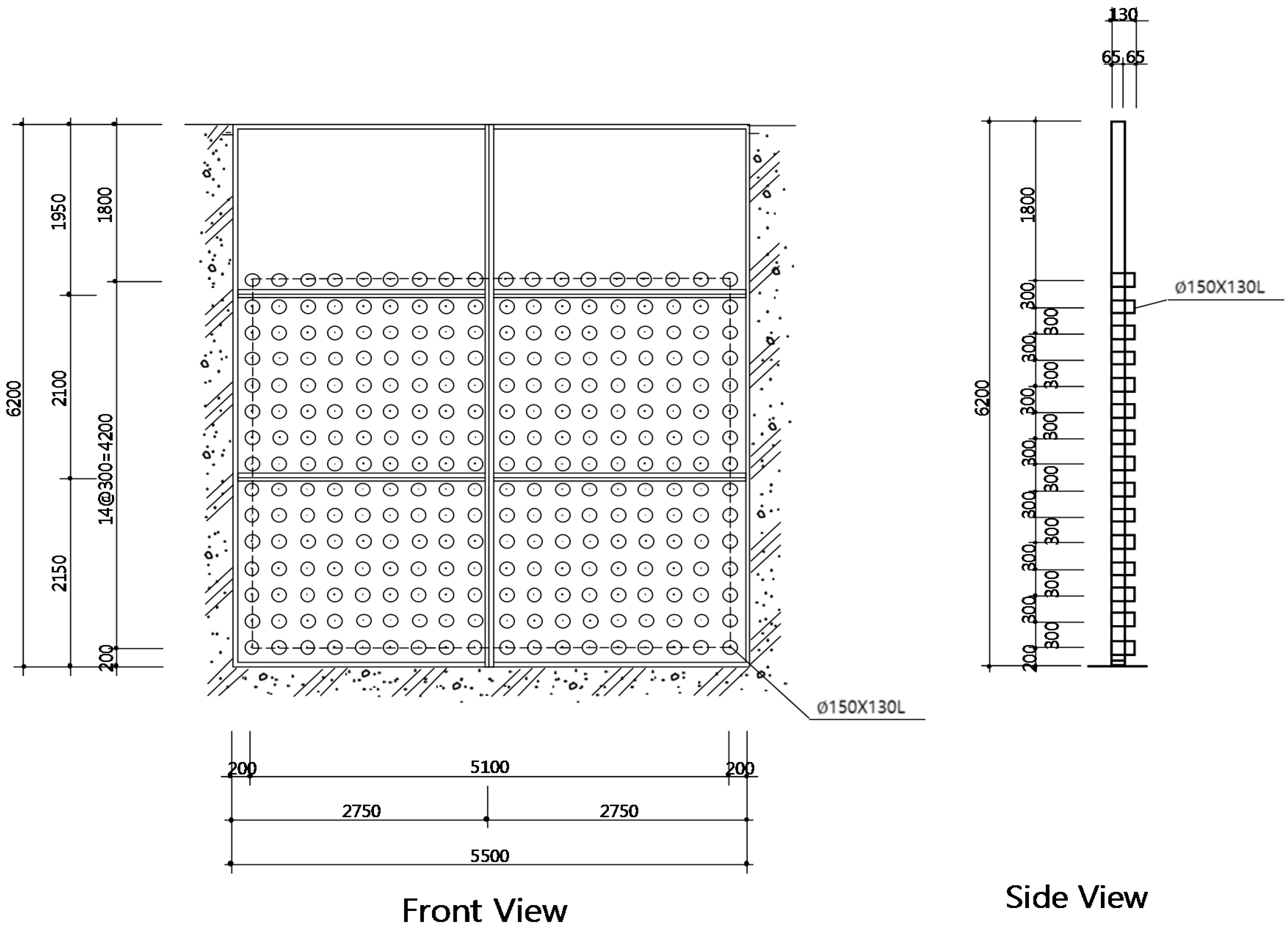
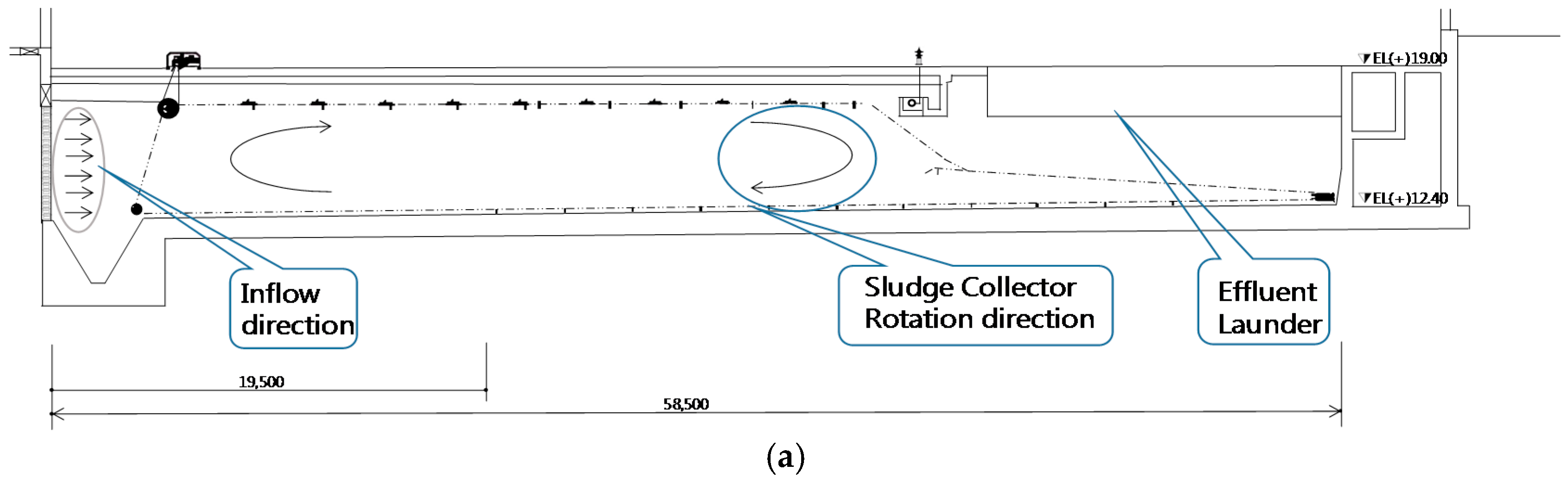
The Suwon Wastewater Treatment Plant owned and operated by Suwon municipal government has two phases: Phases I and II have design capacities of 220,000 m3/d and 300,000 m3/d, respectively. Phase I has circular primary and secondary clarifiers and Phase II has rectangular primary and secondary clarifiers. Most of the influent to the plant is domestic wastewater. Phase II consists of four trains and each train has two bays. Each bay consists of six primary and secondary clarifiers and one bioreactor. At Phase II, wastewater is lifted about 3 m after being passed through the preliminary treatment facility. The lifted and treated wastewater flows into 48 rectangular primary clarifiers and each unit is 30 m long and 6 m wide with an average depth of 3.5 m. The biological treatment process comprises eight bioreactors and 48 secondary clarifiers. The effluents from six primary clarifiers at each bay are combined and passed into a bioreactor. Each bioreactor contains anaerobic, anoxic, and aerobic tanks to biologically remove organic materials, nitrogen, and phosphorus. Three plug-flow passes exist in the bioreactor and each pass is 77 m long and 6 m wide with an average depth of 5.5 m. At each bay, the MLSS from the end of the third pass flows to a transfer channel that splits the MLSS to six secondary clarifiers. Each rectangular clarifier has an inlet perforated wall having 270 holes with 150 mm diameter of each hole and overall opening is 58% of total area, as shown in Figure 1. This wall is to provide equal flow across the clarifier’s cross-section. Figure 2a shows the longitudinal view of the conventional rectangular clarifier. A skimmer flight in each clarifier moves down to the tank bottom at the front end of the effluent weirs and thereafter serves as a sludge collector flight. The sludge collector flight travels counter-currently with respect to the flow through the clarifier. After dumping the accumulated solids to the hopper at the front end of the clarifier, the flight moves up to the water surface and travels co-currently as a skimmer flight. Each clarifier is 58 m long and 6 m wide with an average depth of 5 m and the floor has a slope of 1%. Effluent launders are at the top of the end wall and two side walls stretched from the end of the clarifier to 17.5 m toward the front end. The effluent flows over the V-notch weir on the launders and notch on the weir is on 20 cm centers. Each clarifier has a total weir length of 36 m. The design SOR (Surface Overflow Rate) for this clarifier is 0.74 m/h.
2.2. Physical Description of the Test Clarifier
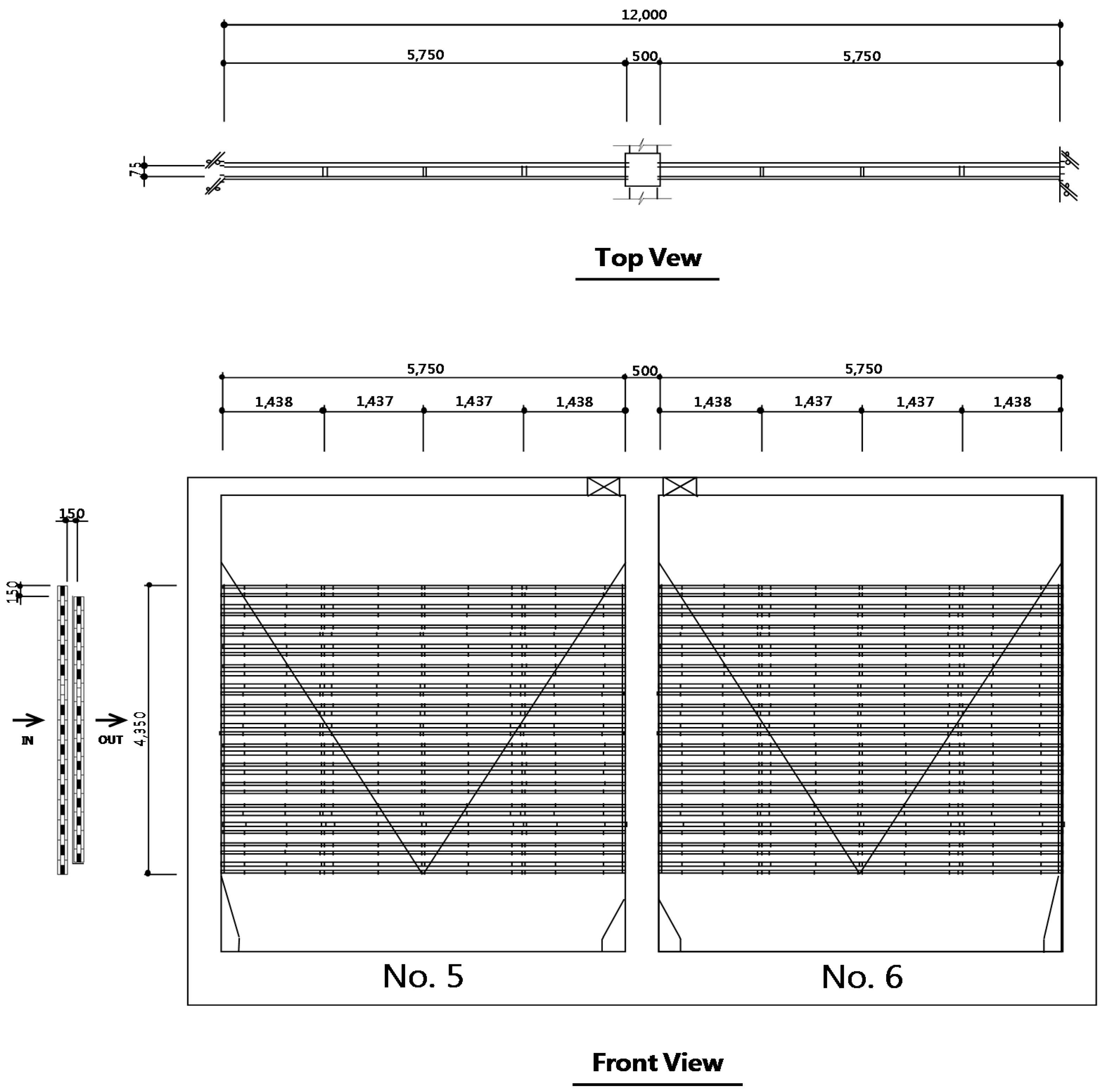
Two double perforated baffles were placed in secondary clarifiers numbered second train, third bay, No. 5 and 6 clarifiers and each clarifier has one baffle. The double perforated baffle contains two vertical slotted baffles where the boards of the first baffle are opposed to the slots of the second baffle, as shown in Figure 3. The first baffle has 15 boards and each board is 5.75 m long and 0.15 m width with a thickness of 5 cm. The boards of the second baffle have the same shape as that of the first baffle and are placed opposed to the slots of the first baffle.
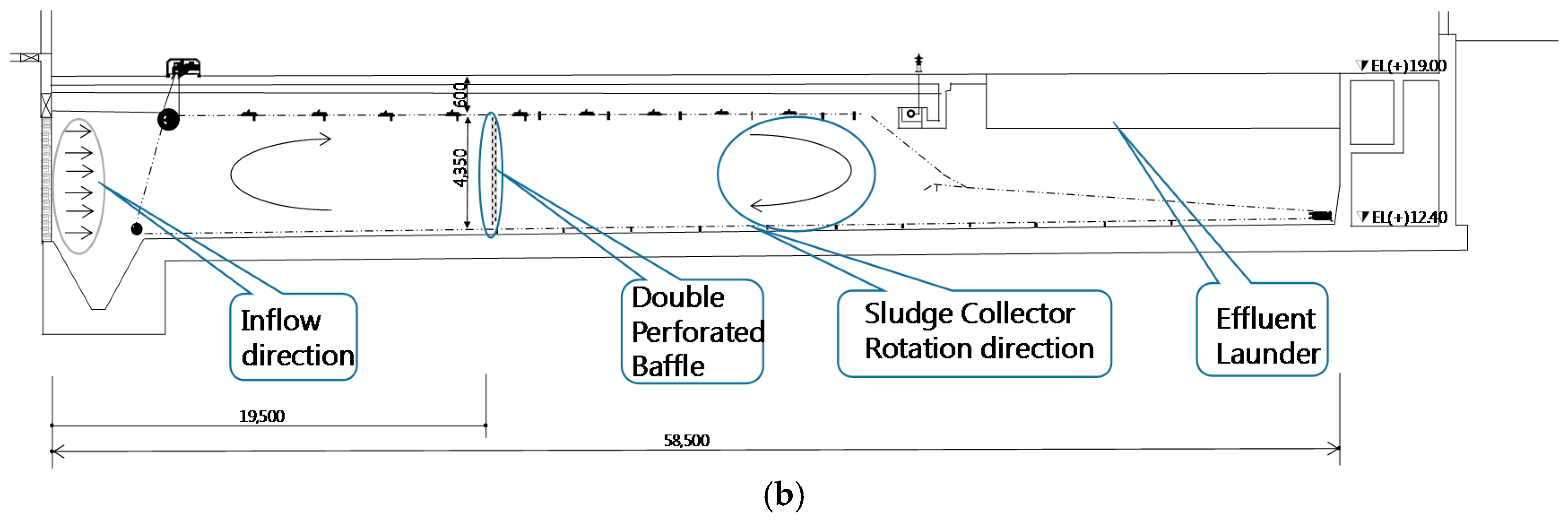
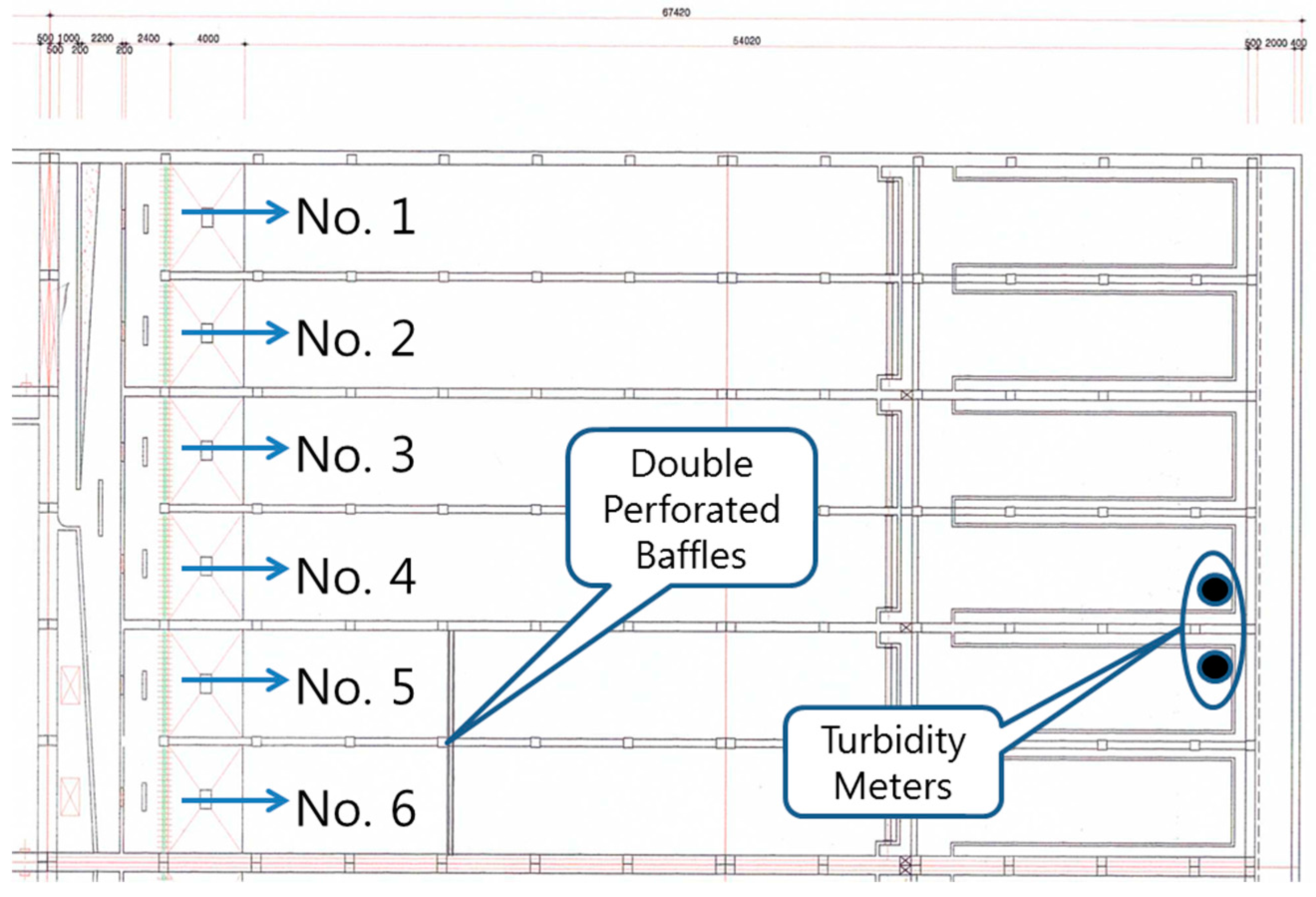
In this study, a double perforated baffle was placed at one-third of the longitudinal length of the clarifier from the inlet to improve the solid removal efficiency by enhancing bio-flocculation and reducing settled sludge shoving by inflow surge (Figure 2b). The effluents from the second train, third bay, No. 5 clarifier that had the baffle (Tank A) and No. 4 clarifier that did not have the baffle (Tank B) were simultaneously tested to determine the effect of the baffle. For the comparison of the effluent quality, turbidity and SS concentrations were measured. An on-line turbidity meter (Model TB-31, DKK-TOA Corporation, Tokyo, Japan) was installed inside the effluent weir of both clarifiers with 60 cm of sensor depth (Figure 4). The turbidity meters were set up to measure turbidity every 5 min and turbidity data were later downloaded to a personal computer via the COM port. Initially, the turbidity and SS measurements were planned for a week every month for one year. However, turbidity measurements were hampered from March to August of 2015 due to the contamination of the turbidity sensor by grease and construction activities in the treatment facility. Starting from September, the experimental period was shortened to a few days because of the manual cleaning of turbidity meter sensors. At each experimental period, grab samples of the effluent from both clarifiers were taken once a day for the SS measurement. The SS was measured according to Standard Methods [23]. Hourly inflow rates to Phase II, MLSS concentrations, and SVI (Sludge Volume Index) of MLSS in the aerobic tank were provided by the plant staff.
3. Results and Discussion
3.1. Computational Fluid Dynamics Model Simulation
The software package developed by McCorquodale et al. [17] was used to simulate the behavior of fluids and solids in the clarifier. For fluids, the equations and constants presented by McCorquodale et al. [17] were used. For solids, the empirical settling equation (Equation (1)) proposed by Takacs et al. [22] was used and the coefficient of K1 was determined by settling tests proposed by Wahlberg [24] and K2 were determined by the simulation study [25], respectively.
where,
Vs = Vo (e−K1(X−Xmin) − e−K2(X−Xmin))
- Vo = Stokes velocity (settling velocity of a single particle in clear water), m/h.
- K1 = empirical coefficient for rapidly settling floc resulting from fit of batch settling data, m3/kg.
- Xmin = the concentrations of non-settling floc, kg/m3.
- K2 = a settling exponent for the poorly settling particles, m3/kg.
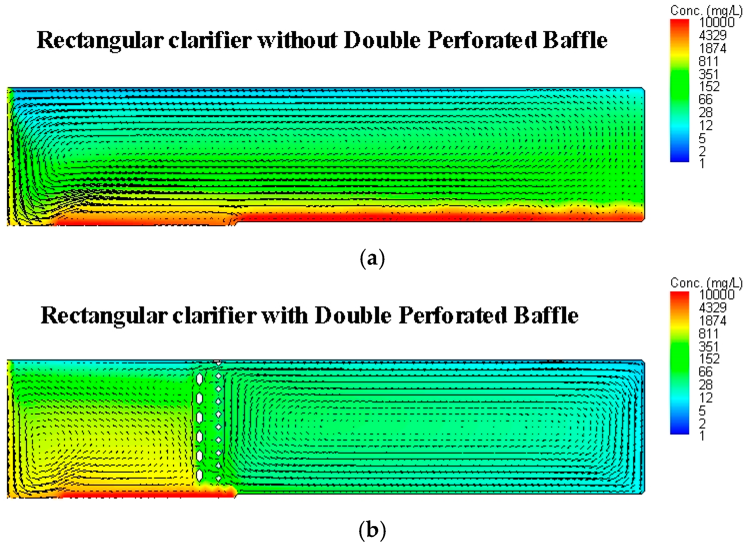
Table 1 shows the coefficients and SS concentrations used to simulate the clarifier. All physical parameters described in Material and Methods and the estimated SORs presented in Figure 6 were used as physical and inflow input data for the simulation, respectively. Figure 5a,b illustrate the simulation results with the SS contours and velocity vector fields of the rectangular clarifier without and with double perforated baffles under constant inflow conditions, respectively. These figures are generated by TecPlot, which imports the output data from the model. The double perforated baffle reduces the velocity and creates turbulence that provides a zone for flocculation. Moreover, the baffle breaks the bottom density current and induces the redistribution of inflow over the clarifier depth. This redistribution creates quiescent conditions that enhance solid settling after the baffle.
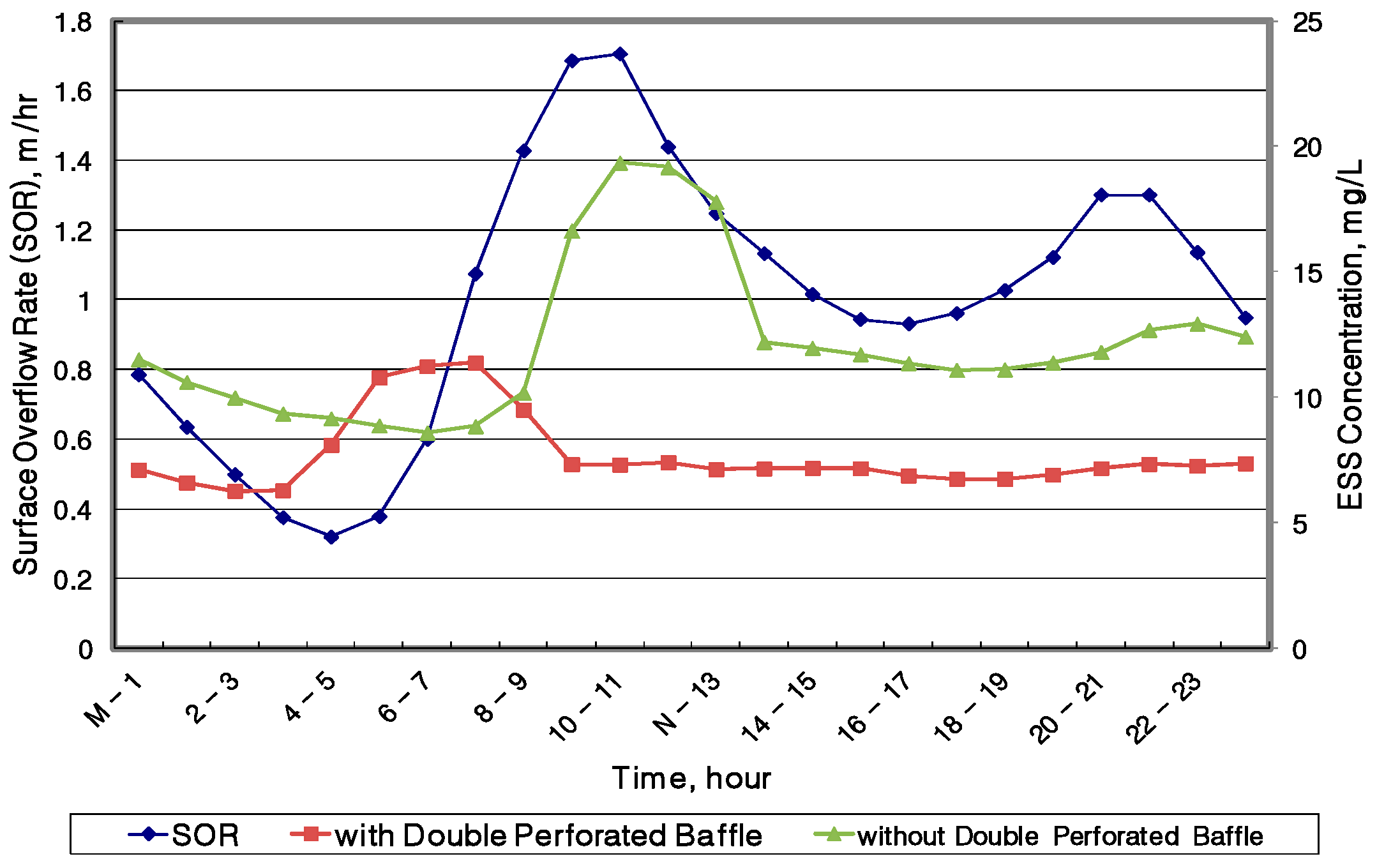
The model proposed by McCorquodale et al. [17] simulates the clarifier under variable inflow conditions. Hourly SORs can be used as input data to determine the effect of changes in inflow on SS removal. Video output is created to display hourly variations of solids and velocity vectors. The video shows the turbulence at the front of the baffle (Figure 5b) and the retardation of longitudinally settled sludge movement caused by high inflow during morning hours. Figure 6 presents the hourly ESS concentration variations along with SORs and shows that ESS concentrations in the clarifier with the baffle are always lower than those in the clarifier without the baffle. The ESS concentrations in the clarifier without the double perforated baffle were proportional to SORs; however, ESS concentrations in the clarifier with the double perforated baffle were relatively constant regardless of SOR changes. Bio-flocculation at the front of the baffle resulted in lower ESS concentrations in the clarifier, with the baffle under various inflow conditions (Figure 6). The reason for high ESS concentrations in the clarifier without the baffle at high SORs is that the high longitudinal velocity created by high SOR pushes the settled sludge to the end of the clarifier and eventually increases ESS concentrations. However, the baffle in the clarifier attenuates the lateral motion of the settled sludge and diminishes the effect of high inflow on ESS concentrations. According to the simulation results, the double perforated baffle must be installed in secondary rectangular clarifiers to achieve low ESS concentrations, if the inherited condition of the wastewater treatment plant that has high inflow fluctuation is considered.
3.2. Experimental Study
As described in Material and Methods, two of the 48 rectangular secondary clarifiers have double perforated baffles; one double perforated baffle in each clarifier. At first, the ESS concentration in the clarifiers with and without double perforated baffles was considered to be a surrogate to understand the effect of baffles on SS removal in rectangular clarifiers. Since the SS test is prone to being unpredictable, especially at low concentrations, and cannot be performed in short intervals, turbidity was chosen as a surrogate described by Walberg [18]. An in-line turbidity meter was installed at the end of the clarifier with the double perforated baffle (Tank A) and without the double perforated baffle (Tank B) to measure turbidity every 5 min. The ESS concentrations in the effluent from both clarifiers were measured once a day during the experiment except for the 20 July measurement. The hourly inflow data during the experiment were obtained from the treatment plant personnel. In the beginning of this study, the effluent turbidity in both clarifiers was measured for one week every month. Turbidity meters were set up to measure and store data every 5 min and the stored data were downloaded to a personal computer later. These downloaded data were compiled to produce hourly average turbidity values compared with the ESS concentrations and the variation of inflow.
Table 2 shows the MLSS concentrations in the aerobic tank, SVIs of MLSS, ESS concentrations of the grab samples in Tanks A and B, sampling times of each grab sample, and effluent turbidity in Tanks A and B at corresponding sampling times. MLSS concentrations and SVIs were provided by the plant personnel and ESS concentrations were measured by the author. SVIs were very low in November and December compared to January, February, and July. The plant personnel explained that DO (Dissolved Oxygen) concentration adjustment in the aerobic tank might contribute to the changes in SVI. Before November, DO concentrations were maintained at 7–8 mg/L to manage operational problems caused by the construction activities around the aerobic tanks and clarifiers. Since all construction work was finished in November, DO concentrations in the aerobic tanks were maintained at 2 mg/L. The plant operator explained that decreasing DO concentrations might have caused low SVI of MLSS.
Table 2 shows that the effluent turbidity in Tank A is consistently lower than that in Tank B except for one case, although the effluent suspended solid concentration in Tank A exceeds the concentration in Tank B in 10 cases out of 25. Wahlberg [19] proposed a relationship between SS and turbidity. In his study, relatively high values of SS concentrations and turbidity were analyzed to present a linear equation of turbidity against SS concentration. The ranges of SS concentrations and turbidity were near 0 to 90 mg/L and 2 to 68 NTU, respectively. However, in this study the relationship between ESS concentrations and the effluent turbidity is not conclusive. The low values of SS concentrations and turbidity as shown in Table 2 may cause this inconclusiveness. The ESS concentrations and turbidity have ranges of 0.4 to 5.5 mg/L and 0.15 to 1.78 NTU, respectively. The sample containing low SS shows inconsistent SS concentration since inclusion and/or exclusion of particles in samples can vary concentrations easily. Since ESS concentrations were not consistent, it was an obvious choice to use turbidity as a surrogate to evaluate the secondary clarifier performance. In Figure 7, Figure 8, Figure 9, Figure 10 and Figure 11, hourly average effluent turbidity in the clarifier with and without double perforated baffles is compared with SORs and the ratios of the effluent turbidity reduction caused by the baffles are presented. The plan was to measure turbidity for one week every month in 2016. While turbidity was accurately measured in January and February, it was unpredictably high from March to June. Discussion with the plant personnel revealed that the effluent from a nearby food waste treatment facility that discharged to the plant for further treatment contained grease that likely attached to the turbidity meter sensor and caused erratically high turbidity values. In order to eliminate the effect of grease on the turbidity meter, the meter’s sensor was manually cleaned starting from July. From August to October, the experiment was halted due to the construction and maintenance activities in the plant. Turbidity and ESS concentration measurements in the effluent from both clarifiers resumed in November and December.
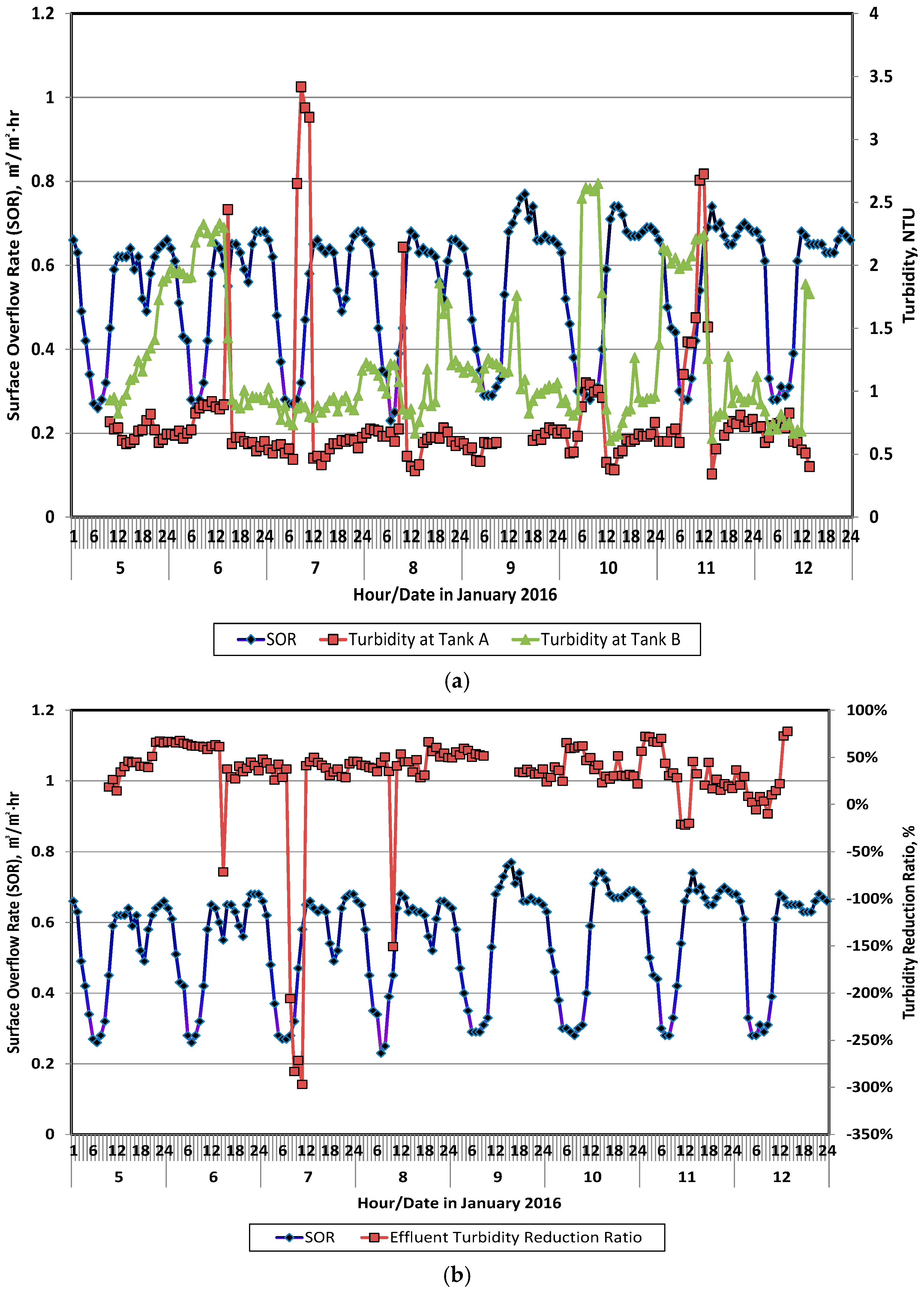
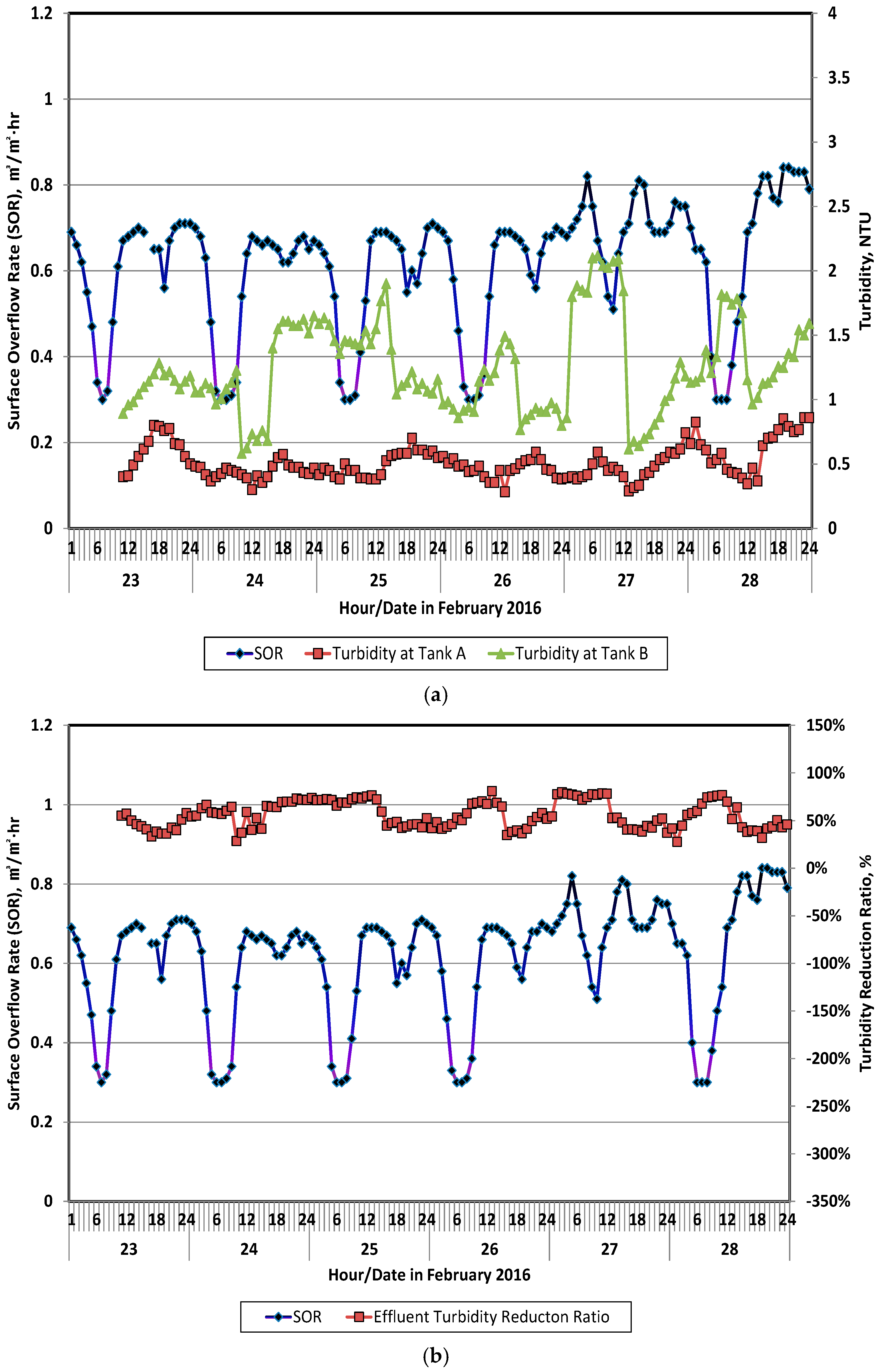
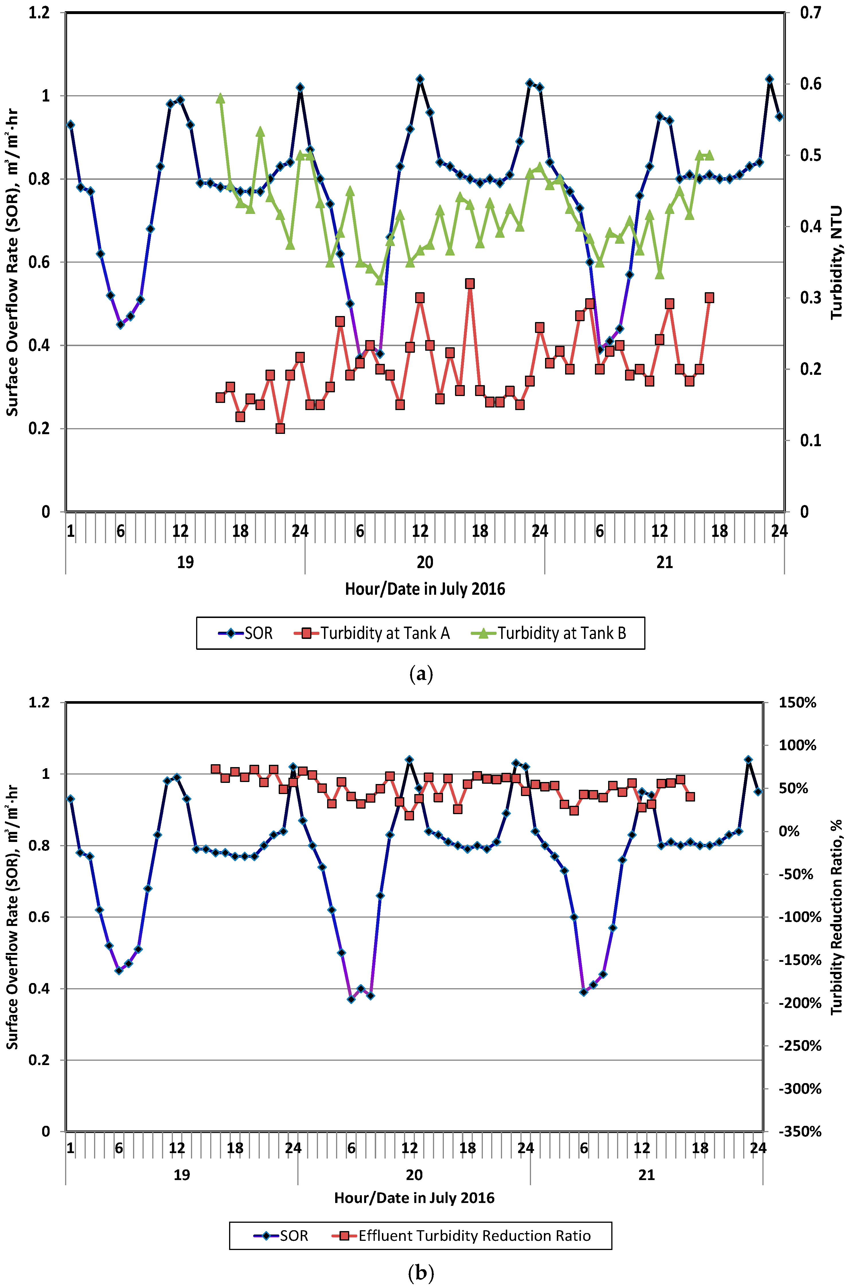
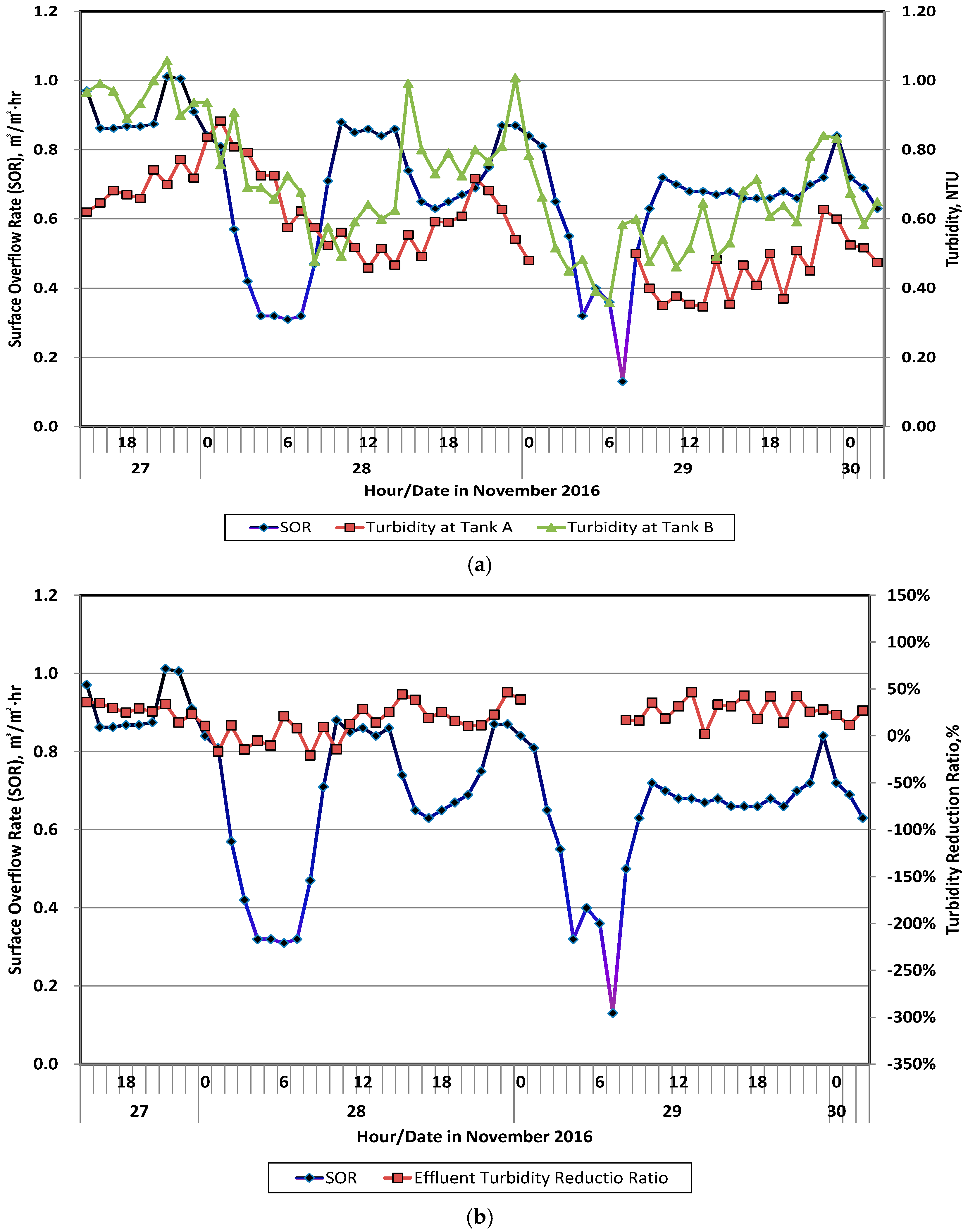
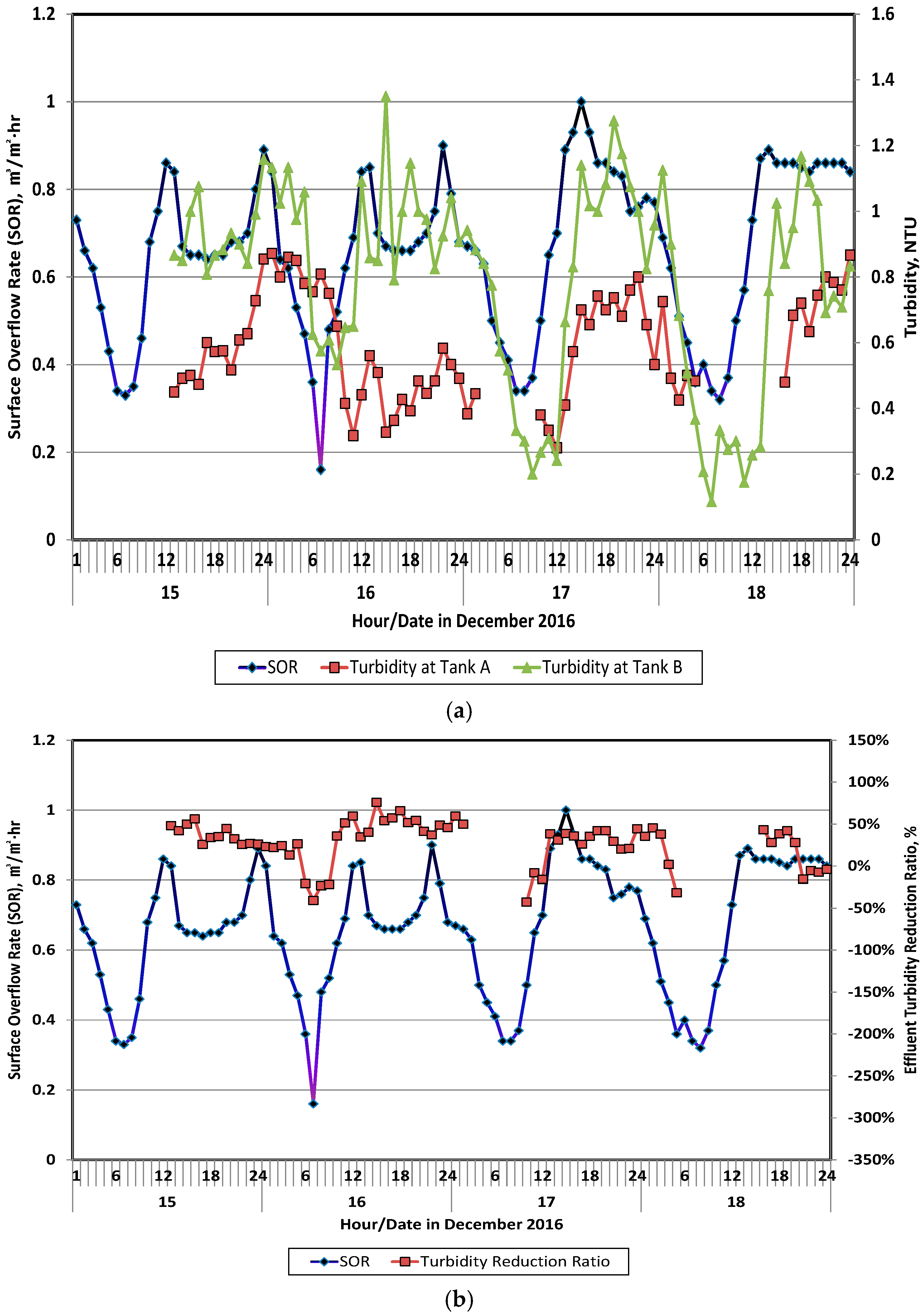
Figure 7a shows hourly average effluent turbidity values in the clarifier with the double perforated baffle as Turbidity in Tank A and without the double perforated baffle as Turbidity in Tank B in January, respectively. SOR represents the hourly surface overflow rate based on the hourly plant inflow. Figure 7b shows the ratios of the effluent turbidity reduction by the baffle. In Figure 7a, the effluent turbidity is proportional to SOR and effluent from the clarifier with the double perforated baffle has less turbidity except for a few cases. The average, maximum, and minimum effluent turbidity values in Tank A were 0.76, 3.42, and 0.34 NTU and in Tank B were 1.22, 2.65, and 0.61 NTU, respectively. Figure 7b shows that the effluent turbidity reduction ratios were not changed significantly by SORs except for a few cases. The average reduction ratio was 30.8% while the maximum and minimum ratios were 77% and −297%, respectively. The minimum value of −297% is likely to be caused by the sensor contamination. Figure 8a,b show the effluent turbidity from Tanks A and B with SORs and effluent turbidity reduction ratios in February, respectively. The effluent turbidity was proportional to SORs in both tanks, while SORs’ influence was more significant in Tank B (Figure 8a). The double perforated baffle played a significant role in reducing the effluent turbidity hike when the SOR surged, consistent with the simulation results presented in Figure 6. The average, maximum, and minimum effluent turbidity values were 0.54, 1.15, and 0.28 NTU in Tank A and 1.25, 2.11 and 0.58 NTU in Tank B, respectively. Figure 8b shows that all effluent turbidity reduction ratios are positive, suggesting that the clarifier with the baffle always has higher solid removal efficiency. Moreover, there was no turbidity sensor contamination during the February experiment. When the elapsed time that inflow flows to the secondary clarifier is considered, the increase in the ratio occurs when the inflow is peaked. The average reduction ratio was 54.0% and the maximum and minimum reduction ratios were 81.0% and 10.4%, respectively. Note that the turbidity sensor had been manually cleaned to eliminate the oil attached to the sensor since July. Figure 9 presents the 48 h experimental data in July. Figure 9a indicates that turbidity in Tank A is always lower than in Tank B and SOR hikes do not affect effluent turbidity as in January and February. The average, maximum, and minimum effluent turbidity values were 0.20, 0.32, and 0.11 NTU in Tank A and 0.41, 0.58, and 0.32 NTU in Tank B, respectively. The maximum effluent turbidity was lower than 1.0 NTU regardless of the baffle installation. The maximum effluent turbidity in Tanks A and B were 3.42 and 2.65 in January and 1.15 and 2.11 NTU in February, respectively. The effluent turbidity in July was very low compared to January and February. Tank A always had lower effluent turbidity than Tank B, suggesting that the perforated baffle plays a role in reducing the effluent turbidity. However, Figure 9a does not show the effluent turbidity hikes in Tank B when SOR increased dramatically as depicted in Figure 7a and Figure 8a. The SOR hike does not likely contribute to the effluent turbidity increase when the effluent turbidity is as low as 0.6 NTU. Figure 9b shows the effluent turbidity reduction ratios in July. There is always a turbidity reduction by the baffle with an average value of 50.4% and SOR change does not contribute to the reduction ratios. Figure 10a,b shows effluent turbidity from Tanks A and B with SORs and effluent turbidity reduction ratios in November, respectively. Figure 10a shows that effluent turbidity is proportional to SOR regardless of the baffle installation. In contrast to Figure 7a and Figure 8a, the effluent turbidity in Tank A is not leveled. Although Tank B has lower effluent turbidity than that of Tank A during the early hours of November 29, Tank A has lower turbidity during most of the experimental period. Higher turbidity in the Tank A effluent may be caused by the contamination of the turbidity sensor since turbidity meters were installed on 27 November and turbidity had been measured before the manual sensor cleaning until 28 November. Tank A having a double perforated baffle has the average, maximum, and minimum effluent turbidity values of 0.57, 0.88, and 0.34 NTU, respectively. Tank B having no double perforated baffles has the average, maximum, and minimum effluent turbidity values of 0.70, 1.05 and 0.36 NTU, respectively. From data from Figure 10a, it is not clear why the baffle in Tank A cannot significantly reduce effluent turbidity when SOR increases (Figure 7a and Figure 8a). The reason could be the range of effluent turbidity or low SVI (Table 2), because the December data had the same SVI range as November; however, turbidity in the Tank A effluent was significantly reduced with high inflow (Figure 11a). Figure 10b shows that SOR does not have any significant role in effluent turbidity reduction ratios. The average reduction ratio was 20.5%. Figure 11a,b shows effluent turbidity in Tanks A and B with SORs and effluent turbidity reduction ratios in December, respectively. Tank A had the average, maximum, and minimum effluent turbidity values of 0.59, 0.87, and 0.28 NTU and Tank B has the values of 0.79, 1.35, and 0.11 NTU, respectively. As in January and February, effluent turbidity was proportional to SORs in December. Although SVI had the same range in December as in November (Table 2), effluent turbidity in Tank A was significantly reduced when SOR increased (Figure 11a), different from the data in November. Figure 11b shows the effluent turbidity reduction ratios by the baffle. The average reduction ratio was 28.1%.
Table 3 presents the average, maximum, and minimum effluent turbidity values in Tanks A and B as well as turbidity reduction ratios in each period, respectively. The average effluent turbidity in Tank A was always lower than that in Tank B although the minimum values of reduction ratios in January, November, and December were negative, suggesting that turbidity in Tank A was higher than that in Tank B. These negative reduction ratios are probably caused by the contamination of the turbidity sensor. Many researchers [7,8,9,10,12,15] claimed that the election of baffles in rectangular clarifiers could reduce the effluent suspended solid concentrations. Bamumer et al. [8] showed that clarifiers with perforated baffles reduced larger amounts of suspended solids and suggested that the multiple installations of perforated baffles could reduce the concentrations of secondary effluent suspended solids to a greater extent. The simulation and experimental results of this study support their claims although two perforated baffles were placed very closely.
The average reduction ratio in November was the lowest (20.5%) and the second lowest was in December (28.1%). SVIs in November and December were significantly lower than those in the other months (Table 2). The overall average turbidity reduction ratio in January, February, and July when SVI of MLSS was less than 100 mL/g was estimated as 45.1%. However, the overall average turbidity reduction ratio in November and December when SVI of MLSS was less than 100 mL/g was estimated as 24.3%. Therefore, the double perforated baffle is less efficient when the MLSS that enters the clarifier has SVI < 100 mL/g. However, these results indicate that the double perforated baffle plays a significant role in decreasing effluent turbidity under any operational conditions. Therefore, double perforated baffles installed in rectangular clarifiers would produce high-quality effluents that would lower the operational costs of downstream filtration units by reducing the backwashing frequency. Fewer backwashes would also lower the hydraulic load to the main stream treatment processes.
Although the double perforated baffle can reduce the overall operational cost of the treatment facility, possible cost saving may not outweigh the installation cost of the baffle. When the baffle is considered, diurnal profile for secondary effluent turbidity along with influent flow must be constructed and overall turbidity reduction by the baffle may be estimated by the results from this study. Based on this estimation, the benefits from the baffle can be accounted against the capital cost of the baffle. Since the double perforated baffle is the permanent structure, the maintenance cost for the baffle may not be considered to analyzing the benefit and cost of the baffle.
4. Conclusions
The performance of rectangular secondary clarifiers with double perforated baffles was evaluated by CFD simulations and field tests. The results are summarized as follows:
The operational data obtained from the field tests are represented well by the CFD simulation results. Simulation results showed lower ESS concentrations in the effluent from the secondary clarifier with the double perforated baffle and the results of the field test were consistent with the simulations with a few exceptions, which might have been caused by the sensor contamination. The double perforated baffle was found to reduce the effluent solids concentrations.
The rectangular secondary clarifier with the hopper at the front end inherits the longitudinal movement of the settled sludge toward the end of the clarifier when high inflow enters the plant. This motion results in high effluent suspended solids concentrations. The double perforated baffle was shown to inhibit the longitudinal movement and decrease the effluent suspended solid concentration hike when high inflow enters the plant.
Since the double perforated baffle can produce low turbidity effluent under any operational conditions, the installation of this baffle in rectangular secondary clarifiers is strongly recommended to reduce the overall operational costs of the filtration units of the wastewater treatment plants.
Acknowledgments
This work was supported by the Kyonggi University Research Grant 2015. The author wishes to acknowledge the help received from Chan-Hui Cho at the Department of Environmental Energy Engineering of the Kyonggi University and Suwon Wastewater treatment plant staff.
Conflicts of Interest
The author declares no conflict of interest and the founding sponsors had no role in the design of the study; in the collection, analyses, or interpretation of data; in the writing of the manuscript, and in the decision to publish the results.
References
- Fischer, A.J.; Hillman, A. Improved Sewage Clarification by Pre-flocculation without Chemicals. Sew. Works J. 1940, 12, 280–306. [Google Scholar]
- Knop, E. Design Studies for the Emscher Mouth Treatment Plant. J. Water Pollut. Control Fed. 1966, 38, 1194–1207. [Google Scholar]
- Parker, D.S. Assessment of Secondary Clarification Design Concepts. J. Water Pollut. Control Fed. 1983, 55, 349–359. [Google Scholar]
- Bender, J.; Crosby, R.M. Project Summary-Hydraulic Characteristics of Activated Sludge Secondary Clarifiers; US EPA: Cincinnati, OH, USA, 1984; pp. 2–3.
- Kawamura, S. Hydraulic Scale-model Simulation of the Sedimentation Process. J. Am. Water Works Assoc. 1981, 73, 372–379. [Google Scholar]
- Lopez, P.R.; Lavin, A.G.; Lopez, M.M.M.; de las Heras, B. Flow Models Rectangular Sedimentation Tanks. Chem. Eng. Process. 2008, 47, 1705–1716. [Google Scholar] [CrossRef]
- Bretscher, U.; Krebs, P.; Hager, W.H. Improvement of Flow in Final Settling Tanks. J. Environ. Eng. 1992, 118, 307–321. [Google Scholar] [CrossRef]
- Krebs, P.; Vischer, D.; Gujer, W. Improvement of Secondary Clarifiers Efficiency by Porous Walls. Water Sci. Technol. 1992, 26, 1147–1156. [Google Scholar]
- Baumer, P.; Volkart, P.; Krebs, P. Dynamic Loading Tests for Final Settling Tank. Water Sci. Technol. 1996, 34, 267–274. [Google Scholar] [CrossRef]
- Ahmed, F.H.; Kamel, A.; Abdel Jawad, S. Experimental Determination of the Optimal Location and Contraction of Sedimentation Tank Baffles. Earth Environ. Sci. 1996, 92, 251–271. [Google Scholar]
- Younes, M.F.; Younes, Y.K.; El-Madah, M.; Ibrahim, I.M.; El-Dannanh, E.H. An Experimental Investigation of Hydrodynamic Damping due to Vertical Baffle Arrangements in a Rectangular Tank. J. Eng. Marit. Environ. 2007, 221, 115–123. [Google Scholar] [CrossRef]
- Kawamura, S. Integrated Design and Operation of Water Treatment Facilities, 2nd ed.; John Wiley and Sons Inc.: New York, NY, USA, 2000; pp. 159–160. [Google Scholar]
- Tamayol, A.; Firoozabadi, B.; Ashjan, M.A. Hydrodynamics of Secondary Settling Tanks and Increasing Their Performance Using Baffles. J. Environ. Eng. 2010, 136, 32–40. [Google Scholar] [CrossRef]
- Asgharzadeh, H.; Frroozabadi, B.; Afshin, H. Experimental Investigation of Effects of Baffle Configurations on the Performance of a Secondary Sedimentation Tank. Sci. Iran. 2011, 18, 938–949. [Google Scholar] [CrossRef]
- Esler, K.E. Optimizing Clarifier Design and Performance. Available online: http://www.wefnet.org/clarifierdesignperform/part1/Optimize.pdf (accessed on 28 April 2017).
- Zhou, S.; Vitasovic, C.; McCorquodale, J.A.; Lipke, S.; DeNicola, M.; Saurer, P. Improving Performance of Large Rectangular Secondary Clarifier. Available online: http://hydrosims.com/files/Optimization_Rectangular_Clarifiers.pdf (accessed on 28 April 2017).
- McCorquoda, J.A.; Griborio, A.; Georgiou, I. Application of a CFD Model to Improve the Performance of Rectangular Clarifiers. In Proceedings of the WEFTEC, Dallas, TX, USA, 26 October 2006; pp. 310–320. [Google Scholar]
- Wahlberg, E.J. Activated Sludge Bioflocculation. Ph.D. Dissertation, Clemson University, Clemson, SC, USA, 1992; pp. 78–175. [Google Scholar]
- Wahlberg, E.J.; Stahl, J.F.; Chen, C.; Augustus, M. Field Application of the Clarifier Research Technical Committee’s Protocol for Evaluating Secondary Clarifier Performance: Rectangular Co-current Sludge Removal Clarifier. In Proceedings of the WEFTEC, Anaheim, CA, USA, 3 October 1993; pp. 554–566. [Google Scholar]
- Asano, T. Wastewater Reclamation and Reuse; Technomic Publishing Company Inc.: Lancaster, PA, USA, 1998; pp. 219–262. [Google Scholar]
- Water Environmental Federation. Clarifier Design, 2nd ed.; McGraw-Hill: New York, NY, USA, 2006; pp. 507–540. [Google Scholar]
- Takacs, I.; Patry, G.G.; Nolasco, D.A. Dynamic Model of the Clarification-Thickening Process. Water Res. 1991, 25, 1263–1271. [Google Scholar] [CrossRef]
- Standard Methods for the Examination of Water and Wastewater. Available online: http://www.umass.edu/mwwp/pdf/sm2540Btotalsolids.PDF (accessed on 4 June 2017).
- Wahlberg, E.J. WERF/CRTC Protocols for Evaluating Secondary Clarifier Performance; Water Environmental Research Foundation: Alexandria, VA, USA, 2001; pp. 5-1–5-34. [Google Scholar]
- Taeyoung Corporation. Performance Evaluation of Double Perforated Baffle in Secondary Clarifiers (2nd Train, 3rd Bay, No. 5, 6); Construction Supervision Report No. Suwon Wastewater 951-594; Taeyoung Corporation: Suwon, Korea, 2015; pp. 2–5. (In Korean) [Google Scholar]
Figure 1.
Inlet perforated wall in the rectangular clarifier for this study. Unit is mm.

Figure 2.
Longitudinal view of the rectangular clarifier (a) without (Tank B) and (b) with a double perforated baffle (Tank A) installed at one-third of the longitudinal length of the clarifier. Unit is mm.
Figure 2.
Longitudinal view of the rectangular clarifier (a) without (Tank B) and (b) with a double perforated baffle (Tank A) installed at one-third of the longitudinal length of the clarifier. Unit is mm.


Figure 3.
Detailed drawings of the double perforated baffle installed in two secondary rectangular clarifiers. Unit is mm.
Figure 3.
Detailed drawings of the double perforated baffle installed in two secondary rectangular clarifiers. Unit is mm.

Figure 4.
Top view of 2nd train 3rd bay rectangular secondary clarifiers and the locations of the double perforated baffles and turbidity meters inserted at the inside of effluent weir with depth of 60 cm. Unit is mm.
Figure 4.
Top view of 2nd train 3rd bay rectangular secondary clarifiers and the locations of the double perforated baffles and turbidity meters inserted at the inside of effluent weir with depth of 60 cm. Unit is mm.

Figure 5.
CFD simulation results showing suspended solid (SS) contours and velocity vector fields in secondary rectangular clarifiers (a) without (Tank B) and (b) with double perforated baffles (Tank A).
Figure 5.
CFD simulation results showing suspended solid (SS) contours and velocity vector fields in secondary rectangular clarifiers (a) without (Tank B) and (b) with double perforated baffles (Tank A).

Figure 6.
CFD simulation results of the rectangular secondary clarifier under diurnal variations of surface overflow rate.
Figure 6.
CFD simulation results of the rectangular secondary clarifier under diurnal variations of surface overflow rate.

Figure 7.
Time series of Surface Overflow Rate (SOR), effluent turbidity in Tanks A and B, and effluent turbidity reduction ratio by the double perforated baffle during the January experimental period. (a) SOR and effluent turbidity in Tanks A and B; (b) Effluent turbidity reduction ratio by the double perforated baffle.

Figure 8.
Time series of SOR, effluent turbidity in Tanks A and B, and effluent turbidity reduction ratio by the double perforated baffle during the February experimental period. (a) SOR and effluent turbidity in Tanks A and B; (b) Effluent turbidity reduction ratio by the double perforated baffle.
Figure 8.
Time series of SOR, effluent turbidity in Tanks A and B, and effluent turbidity reduction ratio by the double perforated baffle during the February experimental period. (a) SOR and effluent turbidity in Tanks A and B; (b) Effluent turbidity reduction ratio by the double perforated baffle.

Figure 9.
Time series of SOR, effluent turbidity in Tanks A and B, and effluent turbidity reduction ratio by the double perforated baffle during the July experimental period. (a) SOR and effluent turbidity in Tanks A and B; (b) Effluent turbidity reduction ratio by the double perforated baffle.
Figure 9.
Time series of SOR, effluent turbidity in Tanks A and B, and effluent turbidity reduction ratio by the double perforated baffle during the July experimental period. (a) SOR and effluent turbidity in Tanks A and B; (b) Effluent turbidity reduction ratio by the double perforated baffle.

Figure 10.
Time series of SOR, effluent turbidity in Tanks A and B, and effluent turbidity reduction ratio by the double perforated baffle during the November experimental period. (a) SOR and effluent turbidity in Tanks A and B; (b) Effluent turbidity reduction ratio by the double perforated baffle.

Figure 11.
Time series of SOR, effluent turbidity in Tanks A and B, and effluent turbidity reduction ratio by the double perforated baffle during the December experimental period. (a) SOR and effluent turbidity in Tanks A and B; (b) Effluent turbidity reduction ratio by the double perforated baffle.


Table 1.
Parameters used in the Computational Fluid Dynamic (CFD) simulation.
| Elements | Value | Remarks |
|---|---|---|
| FSS, kg/m3 | 0.005 | Xmin in Equation (1) |
| ESS, kg/m3 | 0.009 | |
| Vo, m/h | 14.718 | |
| K1, m3/kg | 0.242 | |
| K2, m3/kg | 70.000 | |
| MLSS, kg/m3 | 3.000 |
Table 2.
Mixed Liquor Suspended Solids (MLSS) concentrations, Sludge Volume Index (SVI) and effluent suspended solid concentrations, corresponding effluent turbidity and grab sampling time for suspended solid concentration measurement.
Table 2.
Mixed Liquor Suspended Solids (MLSS) concentrations, Sludge Volume Index (SVI) and effluent suspended solid concentrations, corresponding effluent turbidity and grab sampling time for suspended solid concentration measurement.
| Date | MLSS Concentration in Aerobic Tank mg/L | SVI of MLSS in Aerobic Tank, mL/g | Effluent SS Concentration in Tank A, mg/L | Effluent SS Concentration in Tank B, mg/L | Effluent Turbidity in Tank A, NTU | Effluent Turbidity in Tank B, NTU | Grab Sampling Time |
|---|---|---|---|---|---|---|---|
| 1/6 | 3981 | 178 | 2.2 | 4.0 | 0.58 | 0.93 | 15:27 |
| 1/7 | 3780 | 182 | 2.7 | 4.6 | 0.54 | 0.93 | 15:43 |
| 1/8 | 3764 | 183 | 3.4 | 2.4 | 0.48 | 0.82 | 10:40 |
| 1/10 | 3925 | 158 | 1.3 | 1.4 | 0.43 | 0.86 | 11:43 |
| 1/11 | 3775 | 171 | 1.6 | 2.9 | 0.34 | 0.63 | 13:29 |
| 1/12 | 3728 | 170 | 2.7 | 4.8 | 0.4 | 1.78 | 13:25 |
| 2/23 | 4714 | 165 | 3.5 | 3.9 | 0.41 | 0.96 | 11:00 |
| 2/24 | 4786 | 167 | 3.2 | 2.4 | 0.42 | 0.58 | 9:44 |
| 2/25 | 4800 | 166 | 4.0 | 4.3 | 0.58 | 1.04 | 15:58 |
| 2/26 | 4629 | 161 | 3.0 | 4.8 | 0.50 | 0.77 | 15:01 |
| 2/27 | 4109 | 185 | 4.3 | 3.7 | 0.29 | 0.62 | 12:25 |
| 2/28 | 4313 | 183 | 2.4 | 3.4 | 0.35 | 1.15 | 12:00 |
| 7/19 | 4031 | 136 | 4.0 | 5.5 | 0.86 | 1.48 | 15:15 |
| 7/20 | 4178 | 135 | 1.6 | 1.3 | 0.18 | 0.46 | 16:00 |
| 0.7 | 0.8 | 0.15 | 0.42 | 9:00 | |||
| 1.1 | 0.7 | 0.30 | 0.37 | 11:00 | |||
| 0.7 | 1.2 | 0.16 | 0.42 | 13:00 | |||
| 0.7 | 0.4 | 0.17 | 0.44 | 15:00 | |||
| 0.4 | 1.3 | 0.17 | 0.38 | 17:00 | |||
| 0.6 | 0.4 | 0.15 | 0.39 | 19:00 | |||
| 11/28 | 4288 | 63 | 0.4 | 0.5 | 0.15 | 0.40 | 21:00 |
| 11/29 | 4366 | 62 | 1.4 | 1.3 | 0.56 | 0.49 | 10:37 |
| 12/15 | 4393 | 72 | 1.3 | 1.2 | 0.35 | 0.54 | 10:14 |
| 12/16 | 4370 | 77 | 3.2 | 2.9 | 0.49 | 0.85 | 13:30 |
| 12/17 | 4475 | 80 | 3.2 | 4.0 | 0.51 | 0.85 | 13:20 |
| Mean | 4231 | 141 | 2.1 | 2.6 | 0.38 | 0.74 | |
| Max | 4800 | 185 | 4.3 | 5.5 | 0.86 | 1.78 | |
| Min | 3728 | 62 | 0.4 | 0.4 | 0.15 | 0.37 | |
| SD | 353 | 46 | 1.2 | 1.6 | 0.18 | 0.35 |
Note: Max, Min and SD are Maximum, Minimum and standard deviation, respectively.
Table 3.
Summary of experimental data.
| Month | Elements | Effluent Turbidity in Tank A NTU | Effluent Turbidity in Tank B NTU | Effluent Turbidity Reduction Ratio % |
|---|---|---|---|---|
| January | Average | 0.76 | 1.22 | 30.8 |
| Max | 3.42 | 2.65 | 77.0 | |
| Min | 0.34 | 0.61 | −297.0 | |
| February | Average | 0.54 | 1.25 | 54.0 |
| Max | 1.15 | 2.11 | 81.0 | |
| Min | 0.28 | 0.58 | 10.4 | |
| July | Average | 0.20 | 0.41 | 50.4 |
| Max | 0.32 | 0.58 | 72.4 | |
| Min | 0.11 | 0.32 | 18.2 | |
| November | Average | 0.57 | 0.7 | 20.5 |
| Max | 0.88 | 1.05 | 46.4 | |
| Min | 0.34 | 0.36 | −20.6 | |
| December | Average | 0.59 | 0.79 | 28.1 |
| Max | 0.87 | 1.35 | 75.8 | |
| Min | 0.28 | 0.11 | −42.5 |
© 2017 by the author. Licensee MDPI, Basel, Switzerland. This article is an open access article distributed under the terms and conditions of the Creative Commons Attribution (CC BY) license (http://creativecommons.org/licenses/by/4.0/).
Share and Cite
MDPI and ACS Style
Lee, B. Evaluation of Double Perforated Baffles Installed in Rectangular Secondary Clarifiers. Water 2017, 9, 407. https://doi.org/10.3390/w9060407
AMA Style
Lee B. Evaluation of Double Perforated Baffles Installed in Rectangular Secondary Clarifiers. Water. 2017; 9(6):407. https://doi.org/10.3390/w9060407
Chicago/Turabian StyleLee, Byonghi. 2017. "Evaluation of Double Perforated Baffles Installed in Rectangular Secondary Clarifiers" Water 9, no. 6: 407. https://doi.org/10.3390/w9060407
Note that from the first issue of 2016, this journal uses article numbers instead of page numbers. See further details here.