Beach Response to Wave Forcing from Event to Inter-Annual Time Scales at Grand Popo, Benin (Gulf of Guinea)

 , ,
, ,
Abstract
:1. Introduction
2. Data and Methods
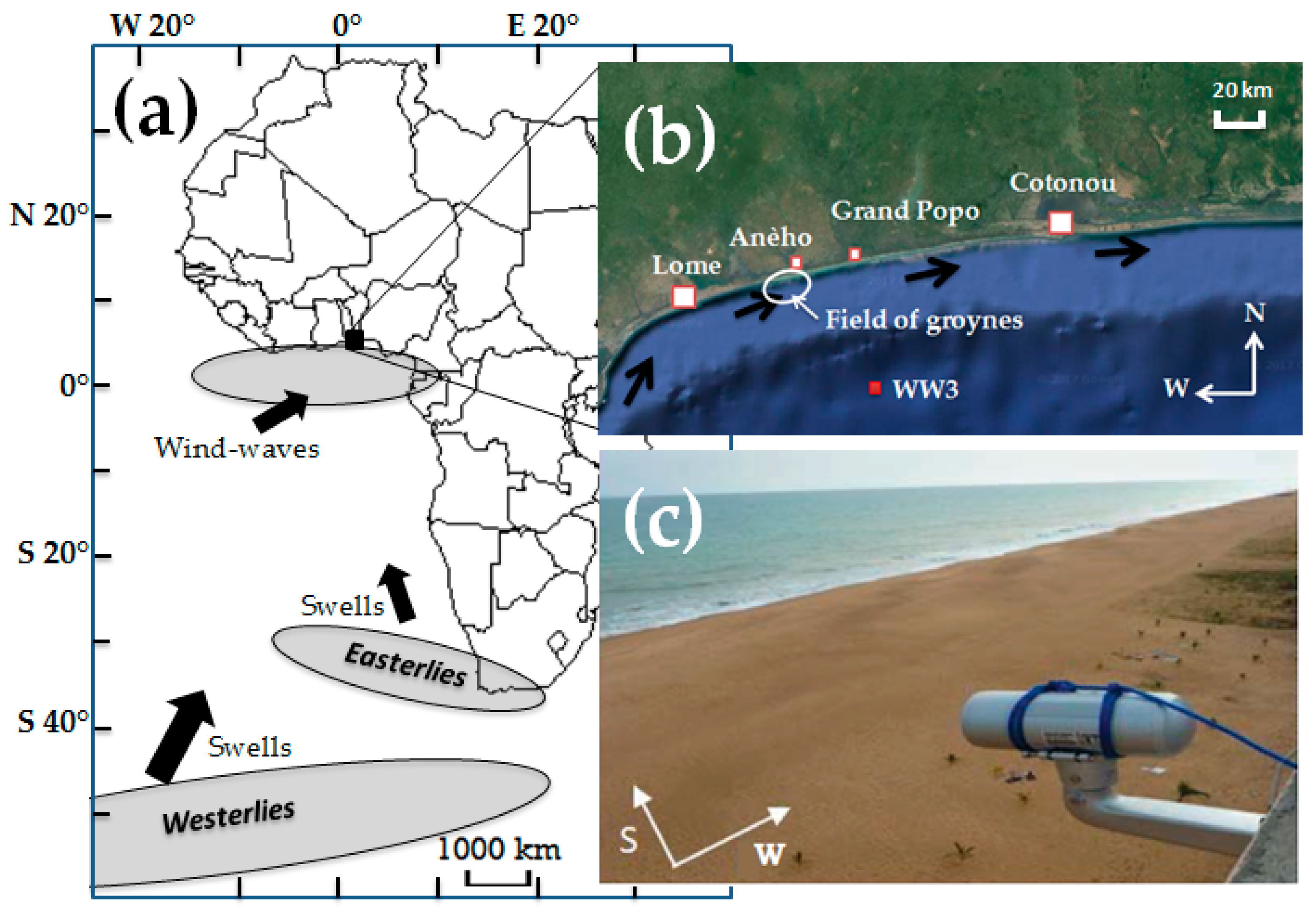
2.1. Study Area
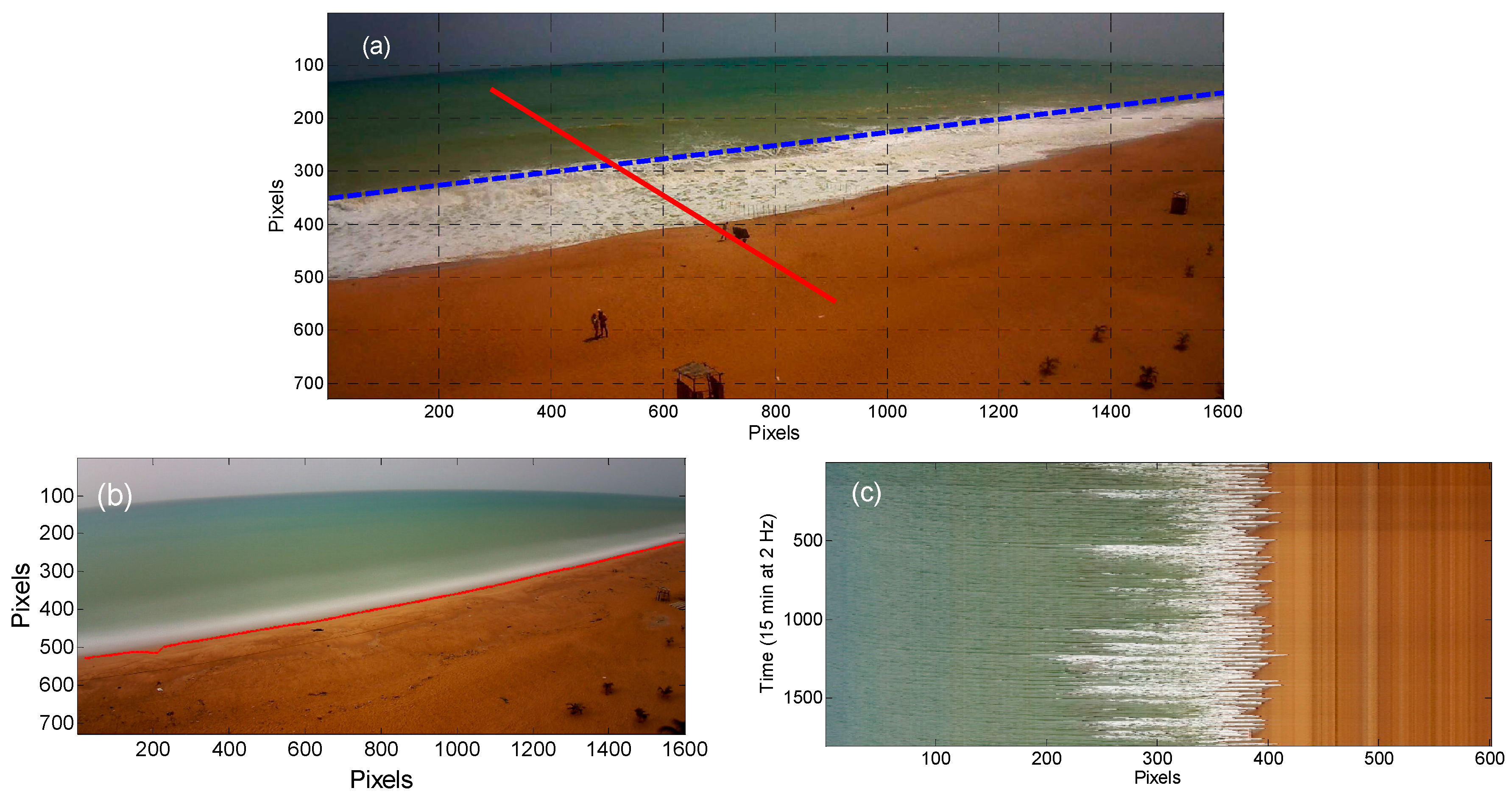
2.2. Video System and Data
2.3. Event Scale: Storms
2.4. Seasonal Signal and Trends
3. Results
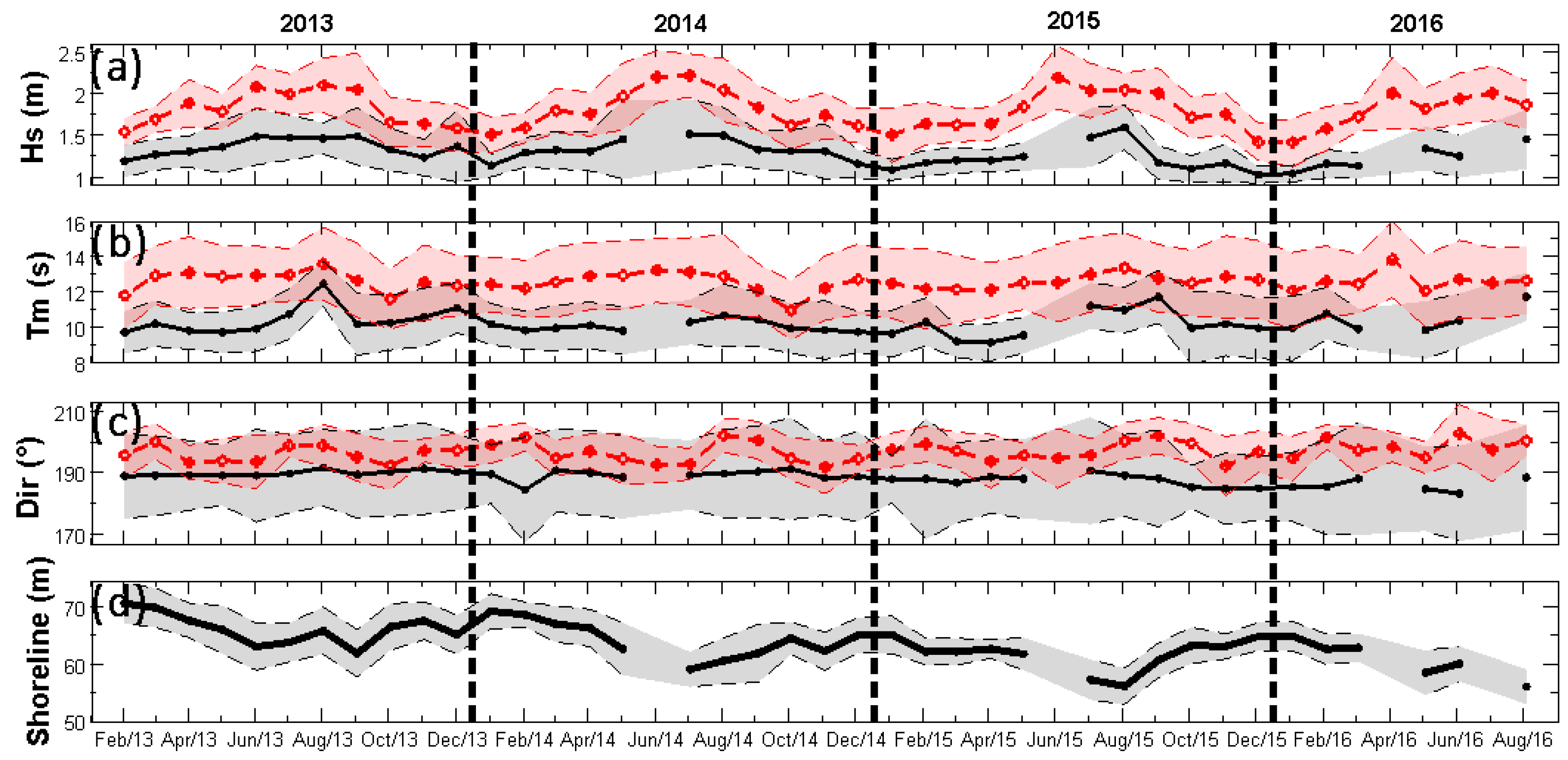
3.1. Hydrodynamic and Morphological Variability
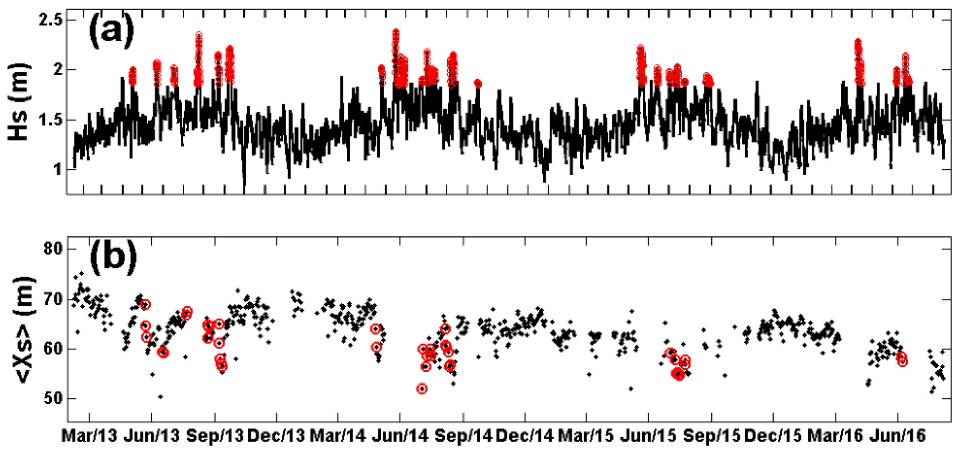
3.2. Storms and Morphological Impact
3.2.1. Detection and Statistics of Individual Storms
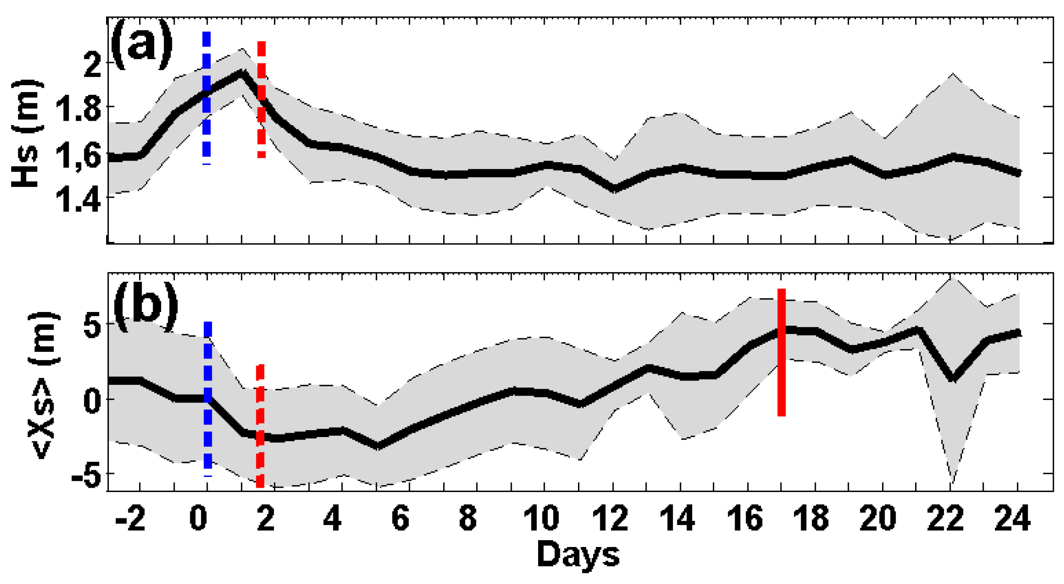
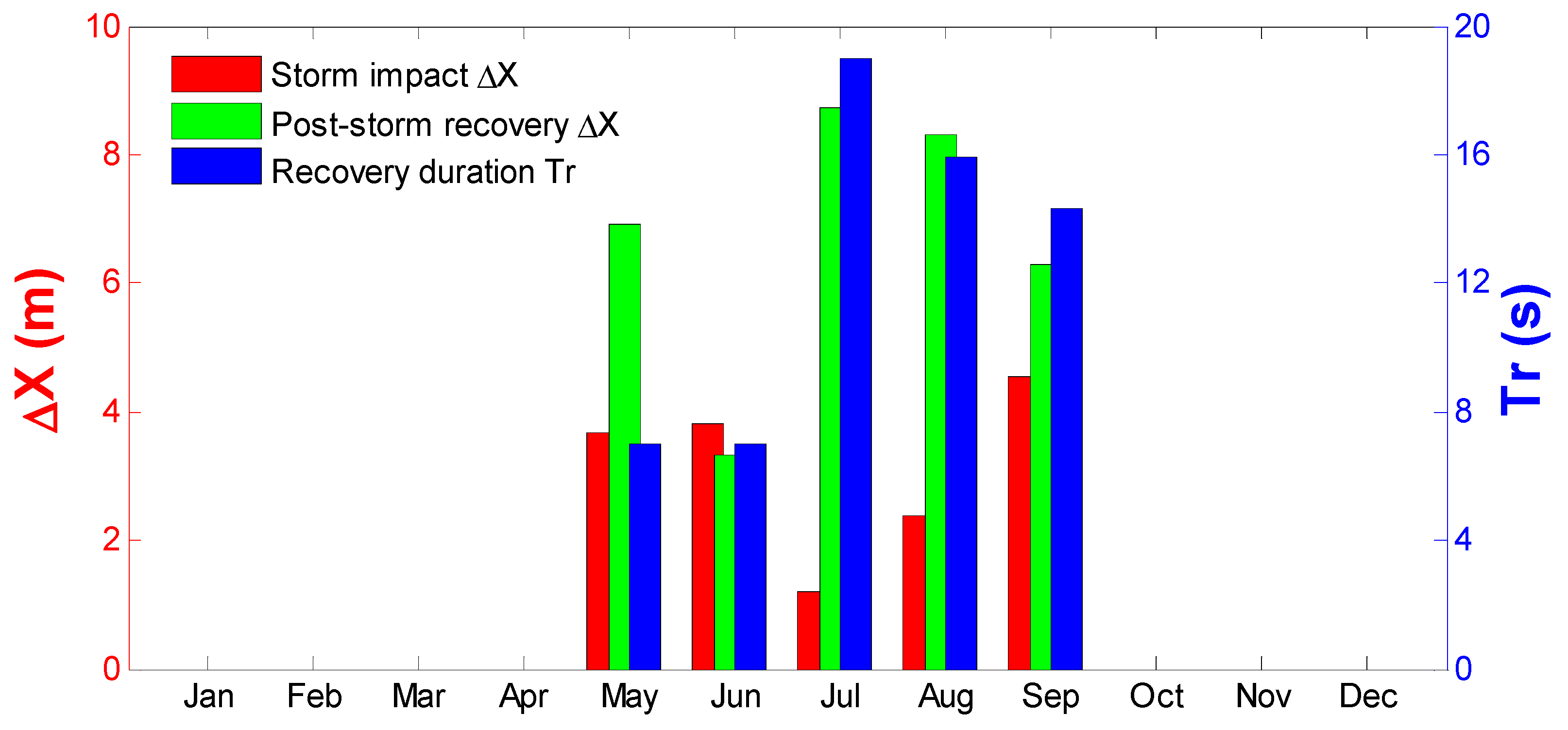
3.2.2. Beach Response to Storms and Resilience
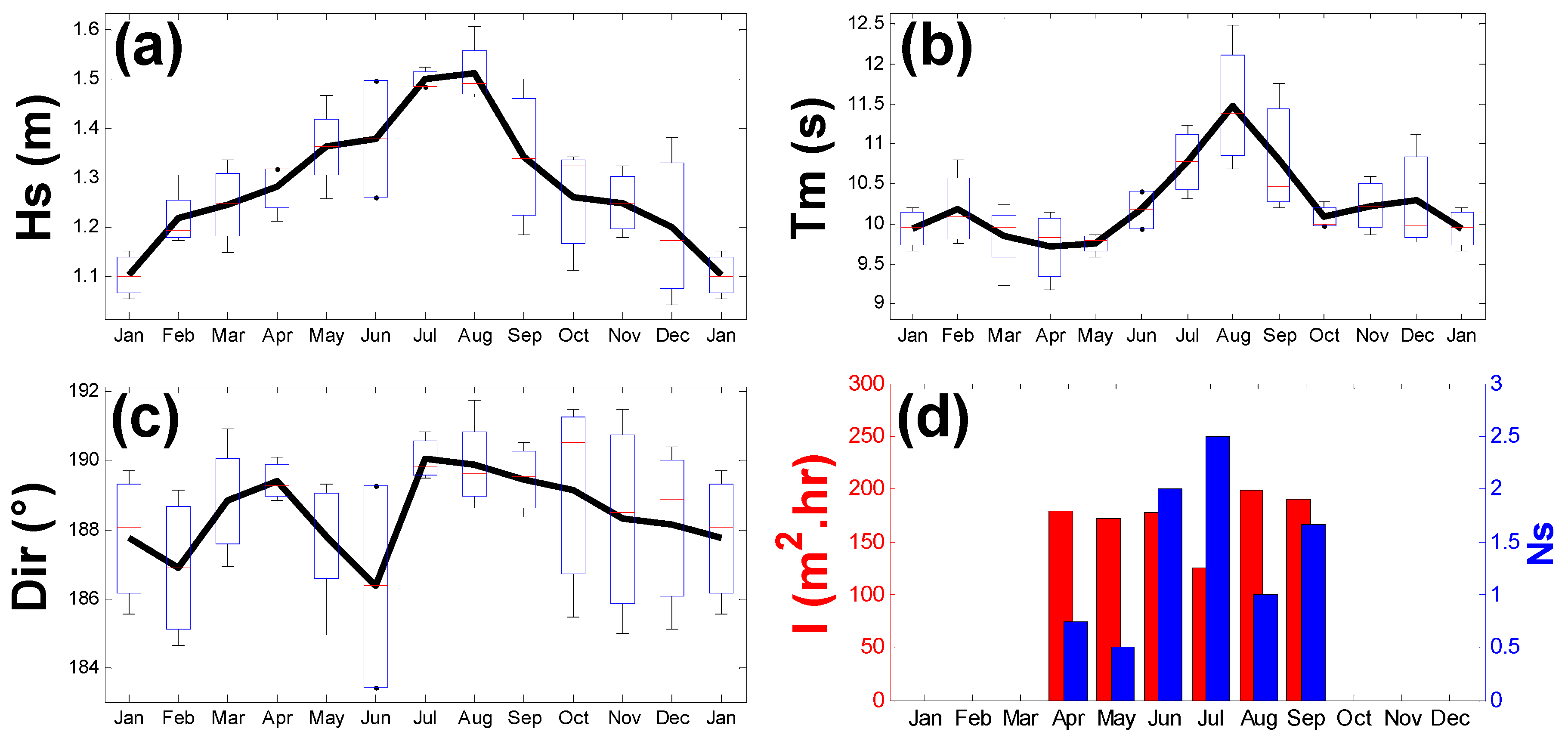
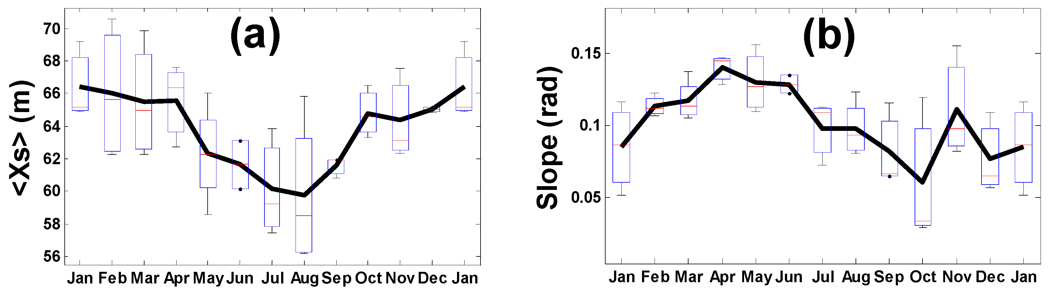
3.3. Seasonal Cycle
3.4. Trends and Inter-Annual Evolution
4. Discussion
5. Conclusions
Acknowledgments
Author Contributions
Conflicts of Interest
References
- Stive, M.J.F.; Aarninkhof, S.G.J.; Hamm, L.; Hanson, H.; Larson, M.; Wijnberg, K.M.; Nicholls, R.J.; Capobianco, M. Variability of shore and shoreline evolution. Coast. Eng. 2002, 47, 211–235. [Google Scholar] [CrossRef]
- Ranasinghe, R.; Callaghan, D.; Stive, M.J.F. Estimating coastal recession due to sea level rise: Beyond the Bruun rule. Clim. Chang. 2012, 110, 561–574. [Google Scholar] [CrossRef]
- Ruggiero, P.; Cote, J.; Kaminsky, G.; Gelfenbaum, G. Scales of variability along the Columbia River littoral cell. In Proceedings of the Coastal Sediments ‘99: The 4th International Symposium on Coastal Engineering and Science of Coastal Sediment Processes, Hauppauge, NY, USA, 21–23 June 1999; pp. 1692–1707. [Google Scholar]
- Brunel, C.; Sabatier, F. Potential influence of sea-level rise in controlling shoreline position on the French Mediterranean Coast. Geomorphology 2009, 107, 47–57. [Google Scholar] [CrossRef]
- Senechal, N.; Coco, G.; Castelle, B.; Marieu, V. Storm impact on the seasonal shoreline dynamics of a meso-to macrotidal open sandy beach (Biscarrosse, France). Geomorphology 2015, 228, 448–461. [Google Scholar] [CrossRef]
- Zhang, K.; Douglas, B.; Leatherman, S. Do storms cause long-term beach erosion along the U.S. East Barrier Coast? J. Geol. 2002, 110, 493–502. [Google Scholar] [CrossRef]
- Morton, R.A.; Paine, J.G.; Gibeaut, J.G. Stages and durations of post-storm beach recovery, southeastern Texas coast, USA. J. Coast. Res. 1994, 10, 884–908. [Google Scholar]
- Morton, R.A.; Gibeaut, J.C.; Paine, J.G. Meso-scale transfer of sand during and after storms: Implications for prediction of shoreline movement. Mar. Geol. 1995, 126, 161–179. [Google Scholar] [CrossRef]
- Castelle, B.; Marieu, V.; Bujan, S.; Splinter, K.D.; Robinet, A.; Senechal, N.J.; Ferreira, S. Impact of the winter 2013–2014 series of severe Western Europe storms on a double-barred sandy coast: Beach and dune erosion and megacusp embayments. Geomorphology 2015, 238, 135–148. [Google Scholar] [CrossRef]
- Masselink, G.; Scott, T.; Russel, P.; Davidson, M.A.; Conley, D.C. The extreme 2013/2014 winter storms: Hydrodynamic forcing and coastal response along the southwest coast of England. Earth Surf. Process. Landf. 2015, 41, 378–391. [Google Scholar] [CrossRef]
- Almeida, L.P.; Vousdoukas, M.V.; Ferreira, Ó.; Rodrigues, B.A.; Matias, A. Thresholds for storm impacts on an exposed sandy coastal area in southern Portugal. Geomorphology 2012, 143, 3–12. [Google Scholar] [CrossRef]
- Angnuureng, D.B.; Almar, R.; Senechal, N.; Castelle, B.; Addo, K.A.; Marieu, V.; Ranasinghe, R. Shoreline resilience to individual storms and storm clusters on a meso-macrotidal barred beach. Geomorphology 2017, 290, 265–276. [Google Scholar] [CrossRef]
- Ba, A.; Senechal, N. Extreme winter storm versus summer storm: Morphological impact on a sandy beach. J. Coast. Res. 2013, 1, 648–653. [Google Scholar] [CrossRef]
- Laibi, R.; Anthony, E.; Almar, R.; Castelle, B.; Senechal, N.; Kestenare, E. Longshore drift cell development on the human-impacted Bight of Benin sand barrier coast, West Africa. J. Coast. Res. 2014, 70, 78–83. [Google Scholar] [CrossRef]
- Almar, R.; Kestenare, E.; Reyns, J.; Jouanno, J.; Anthony, E.J.; Laibi, R.; Hemer, M.; Du Penhoat, Y.; Ranasinghe, R. Response of the Bight of Benin (Gulf of Guinea, West Africa) coastline to anthropogenic and natural forcing, Part1: Wave climate variability and impacts on the longshore sediment transport. Cont. Shelf Res. 2015, 110, 48–59. [Google Scholar] [CrossRef]
- Anthony, E.J.; Blivi, A.B. Morphosedimentary evolution of a delta-sourced, drift-aligned sand barrier–lagoon complex, western Bight of Benin western Bight of Benin. Mar. Geol. 1999, 158, 161–176. [Google Scholar] [CrossRef]
- Yates, M.L.; Guza, R.T.; O’Reilly, W.C. Equilibrium shoreline response: Observations and modeling. Geophys. Res. 2009, 114. [Google Scholar] [CrossRef]
- Abessolo, O.G.; Almar, R.; Kestenare, E.; Bahini, A.; Houngue, G.H.; Jouanno, J.; Du Penhoat, Y.; Castelle, B.; Melet, A.; Meyssignac, B.; et al. Potential of video cameras in assessing event and seasonal coastline behaviour: Grand Popo, Benin (Gulf of Guinea). J. Coast. Res. 2016, 442–446. [Google Scholar] [CrossRef]
- Degbe, C.G.E.; Laibi, R.; Sohou, Z.; Oyede, M.L.; Du Penhoat, Y.; Djara, M.B. Diachronic analysis of coastline evolution between Grand-Popo and Hillacondji (Benin), from 1984 to 2011. Water 2016. submitted. [Google Scholar]
- Almar, R.; Ibaceta, R.; Blenkinsopp, C.; Catalan, P.; Cienfuegos, R.; Viet, N.T.; Duong Hai, T.; Uu, D.V.; Lefebvre, J.P.; Laryea, W.S.; et al. Swash-based wave energy reflection on natural Beaches. In Proceedings of the Coastal Sediments 2015, San Diego, CA, USA, 11–15 May 2015. [Google Scholar]
- Wright, L.D.; Short, A.D. Morphodynamic variability of surf zones and beaches: A synthesis. Mar. Geol. 1984, 56, 93–118. [Google Scholar] [CrossRef]
- Almar, R.; Honkonnou, N.; Anthony, E.J.; Castelle, B.; Senechal, N.; Laibi, R.; Mensah-Senoo, T.; Degbe, G.; Quenum, M.; Dorel, M.; et al. The Grand Popo beach 2013 experiment, Benin, West Africa: From short timescale processes to their integrated impact over long-term coastal evolution. J. Coast. Res. 2014, 651–656. [Google Scholar] [CrossRef]
- Angnuureng, D.B.; Almar, R.; Addo, K.A.; Castelle, B.; Senechal, N.; Laryea, S.W.; Wiafe, G. Video observation of waves and shoreline change on the Microtidal James Town Beach in Ghana. J. Coast. Res. 2016, 1022–1026. [Google Scholar] [CrossRef]
- Holland, K.T.; Holman, R.A.; Lippmann, T.C. Practical use of video imagery in near-shore oceanographic field studies. IEEE J. Ocean. Eng. 1997, 22, 81–92. [Google Scholar] [CrossRef]
- Almar, R.; Ranasinghe, R.; Senechal, N.; Bonneton, P.; Roelvink, D.; Bryan, K.; Marieu, V.; Parisot, J.P. Video-based detection of shorelines at Complex Meso–Macro Tidal Beaches. J. Coast. Res. 2012, 28, 1040–1048. [Google Scholar] [CrossRef]
- Almar, R.; Cienfuegos, R.; Catalán, P.A.; Michallet, H.; Castelle, B.; Bonneton, P.; Marieu, V. A new breaking wave height direct estimator from video imagery. Coast. Eng. 2012, 61, 42–48. [Google Scholar] [CrossRef]
- Almar, R.; Senechal, N.; Bonneton, P.; Roelvink, D. Wave celerity from video imaging: A new method. Proceedings of Coastal Engineering 2008, Hamburg, Germany, 31 August–5 September 2008; pp. 661–673. [Google Scholar]
- Almar, R.; Michallet, H.; Cienfuegos, R.; Bonneton, P.; Ruessink, B.G.; Tissier, M. On the use of the radon transform in studying nearshore wave dynamics. Coast. Eng. 2014, 92, 24–30. [Google Scholar] [CrossRef]
- Rascle, N.; Ardhuin, F. Global wave parameter data base for geophysical applications. Part II: Model validation with improves source term parameterization. Ocean Model. 2013, 70, 145–151. [Google Scholar] [CrossRef]
- Larson, M.; Hoan, L.X.; Hanson, H. Direct formula to compute wave height and angle at incipient breaking. J. Waterw. Port Coast. Ocean Eng. 2010, 136, 119–122. [Google Scholar] [CrossRef]
- Boak, E.H.; Turner, I.L. Shoreline definition and detection: A review. J. Coast. Res. 2005, 21, 688–703. [Google Scholar] [CrossRef]
- Aarninkhof, S.G.J.; Turner, I.L.; Dronkers, D.T.; Caljouw, M.; Nipius, L. A video-based technique for mapping intertidal beach bathymetry. Coast. Eng. 2003, 49, 275–289. [Google Scholar] [CrossRef]
- Hamed, K.H.; Rao, A.R. A modified Mann-Kendall trend test for autocorrelated data. J. Hydrol. 1998, 204, 182–196. [Google Scholar] [CrossRef]
- Tolman, H.L. Limiters in third-generation wind wave models. Glob. Atmos. Ocean Syst. 2002, 8, 67–83. [Google Scholar] [CrossRef]
- Woodcock, F.; Greenslade, D.J.M. Consensus of numerical model forecasts of significant wave heights. Weather Forecast. 2007, 22, 792–803. [Google Scholar] [CrossRef]
- Ranasinghe, R.; Holman, R.; de Schipper, M.A.; Lippmann, T.; Wehof, J.; Minh Duong, T.; Roelvink, D.; Stive, M.J.F. Quantification of nearshore morphological recovery time scales using Argus video imaging: Palm Beach, Sydney and Duck, NC. Coast. Eng. Proc. 2012, 1, 24. [Google Scholar]


| Video–WW3 | Hs (m) | Tm (s) | Dir (°) |
|---|---|---|---|
| Correlation | 0.8 | 0.4 | 0.2 |
| RMSE | 0.3 | 2.4 | 9.4 |
| ME | 0.3 | 2.3 | 8.5 |
| Study Period | 2013 | 2014 | 2015 | 2016 (January–August) | ||||
|---|---|---|---|---|---|---|---|---|
| Mean | Mean | Mean | Mean | |||||
| Hs (m) | 1.35 | +0.05 | 1.34 | +0.04 | 1.23 | −0.07 | 1.28 | −0.06 |
| Tm (s) | 10.4 | +0.2 | 10.1 | −0.2 | 10.2 | −0.1 | 10.6 | +0.3 |
| Dir (°) | 188.9 | +1.4 | 188.2 | +0.5 | 186.4 | −1.3 | 185.2 | −1.8 |
| Shoreline position (m) | 66.4 | +2.8 | 63.9 | +0.2 | 61.8 | −1.9 | 60.1 | −2.9 |
| Beach slope (rad) | 0.098 | −0.006 | 0.101 | 0 | 0.109 | +0.008 | 0.113 | −0.04 |
© 2017 by the authors. Licensee MDPI, Basel, Switzerland. This article is an open access article distributed under the terms and conditions of the Creative Commons Attribution (CC BY) license (http://creativecommons.org/licenses/by/4.0/).
Share and Cite
Abessolo Ondoa, G.; Bonou, F.; Tomety, F.S.; Du Penhoat, Y.; Perret, C.; Degbe, C.G.E.; Almar, R. Beach Response to Wave Forcing from Event to Inter-Annual Time Scales at Grand Popo, Benin (Gulf of Guinea). Water 2017, 9, 447. https://doi.org/10.3390/w9060447
Abessolo Ondoa G, Bonou F, Tomety FS, Du Penhoat Y, Perret C, Degbe CGE, Almar R. Beach Response to Wave Forcing from Event to Inter-Annual Time Scales at Grand Popo, Benin (Gulf of Guinea). Water. 2017; 9(6):447. https://doi.org/10.3390/w9060447
Chicago/Turabian StyleAbessolo Ondoa, Grégoire, Frédéric Bonou, Folly Serge Tomety, Yves Du Penhoat, Clément Perret, Cossi Georges Epiphane Degbe, and Rafael Almar. 2017. "Beach Response to Wave Forcing from Event to Inter-Annual Time Scales at Grand Popo, Benin (Gulf of Guinea)" Water 9, no. 6: 447. https://doi.org/10.3390/w9060447