Evaluating Annual Maximum and Partial Duration Series for Estimating Frequency of Small Magnitude Floods


1
CSIRO Land and Water Flagship, Commonwealth Scientific and Industrial Research Organisation, Canberra, ACT 2601, Australia
2
Integrated Catchment Assessment and Management (iCAM) Centre, The Australian National University, Canberra, ACT 2601, Australia
3
CSIRO Land and Water Flagship, Commonwealth Scientific and Industrial Research Organisation, Glen Osmond, SA 5064, Australia
*
Author to whom correspondence should be addressed.
Water 2017, 9(7), 481; https://doi.org/10.3390/w9070481
Submission received: 1 May 2017
/
Revised: 22 June 2017
/
Accepted: 24 June 2017
/
Published: 30 June 2017
Abstract
:Understanding the nature of frequent floods is important for characterising channel morphology, riparian and aquatic habitat, and informing river restoration efforts. This paper presents results from an analysis on frequency estimates of low magnitude floods using the annual maximum and partial series data compared to actual flood series. Five frequency distribution models were fitted to data from 24 gauging stations in the Great Barrier Reef (GBR) lagoon catchments in north-eastern Australia. Based on the goodness of fit test, Generalised Extreme Value, Generalised Pareto and Log Pearson Type 3 models were used to estimate flood frequencies across the study region. Results suggest frequency estimates based on a partial series are better, compared to an annual series, for small to medium floods, while both methods produce similar results for large floods. Although both methods converge at a higher recurrence interval, the convergence recurrence interval varies between catchments. Results also suggest frequency estimates vary slightly between two or more partial series, depending on flood threshold, and the differences are large for the catchments that experience less frequent floods. While a partial series produces better frequency estimates, it can underestimate or overestimate the frequency if the flood threshold differs largely compared to bankfull discharge. These results have significant implications in calculating the dependency of floodplain ecosystems on the frequency of flooding and their subsequent management.
1. Introduction
Flood frequency estimates are of prime importance in many water resource planning and management projects such as design of infrastructure, flood insurance studies, floodplain management and ecological studies [1,2]. In the past, research on flood frequency has focused on the estimation of extreme flood events because of their large and often dramatic impacts on society and visible economic costs. Conversely, the importance of frequent, low-magnitude floods is often overlooked. For example, despite their high erosive power, large floods transport a relatively small proportion of total sediment loads to the marine environment because they occur less frequently. In many catchments, floods occurring on average once a year account for 50% of total sediment loads [3]. While large floods are usually responsible for channel avulsions, levee breaches, and transporting large bed-load sediments, frequent floods (e.g., recurrence interval of one or two years) are primarily responsible for controlling channel morphology because of their frequent nature and ability to erode and transport large volumes of fine sediment. Frequent floods are especially important for riparian and aquatic biodiversity [4,5,6,7,8]. Frequent, low-magnitude floods also indirectly shape communities by acting as a disturbance agent by altering nutrient distribution, rearranging sediment and removing individual organisms, creating patchiness that fosters biodiversity [9]. Furthermore, comparatively frequent floods that overtop channel banks provide a connection between the river and its floodplain, exchanging nutrients, organisms, and sediment [4,10,11]. Recognising the geomorphic and ecological importance of high-frequency floods, river restoration practitioners have identified floods with recurrence intervals typically in the range of one to two years as an important consideration in channel design criteria [12]. Given the significance of high-frequency floods for channel morphology, ecology, and restoration, changes in flood regimes will have important implications for channel process, function, and management.
Previous studies used both the annual maximum (AM) and peak over threshold (POT) series (commonly known as partial series) to estimate flood frequency in Australia (e.g., [13,14,15]) and elsewhere (e.g., [16,17,18]). The advantage of the AM series is that flood events can be considered independent, flood data can be extracted easily and frequency distributions generally conform to theoretical distributions. The advantage of the POT series is that it produces more data points, which are particularly useful when the period of stream-flow record is short. The Institution of Engineers Australia (IEA) recommends the use of the POT series for estimating the magnitude of small floods as it provides better estimates of frequent floods [19]. However, the use of the partial series has been less popular because of the complexity in choosing the threshold above which a flow is designated to be a flood [20,21]. As there is no unique threshold value which best defines the partial series, an iterative approach is generally used [22,23]. Typically, small flood thresholds increase the number of events designated as being floods, providing a larger statistical sample that may improve flood frequency estimates. However, as the number of flood events increase, the likelihood that they will be independent decreases. Because of greater computational convenience and avoidance of dependence between floods, AM series are often preferred over POT series. However, none of the previous studies evaluated estimates of the AM and POT series compared to an actual flood series.
The main contribution of this study to the international literature is to quantify bankfull discharge and build an actual flood series for an individual catchment. This information can be used to assign flood threshold values in the POT approach, thereby reducing one of the key sources of uncertainty in using this approach. Reducing the uncertainty in assigning flood thresholds using the POT approach provides a firm basis for better understanding differences in the results from the annual and partial series methods. Findings of this study will greatly improve flood frequency estimates for low magnitude floods in catchments adjacent to the Great Barrier Reef (GBR) lagoon and the method is applicable to any river catchment across the world. This manuscript is structured as follows: Section 2 describes the study area and methods. The results of this study are presented in Section 3 and a discussion is provided in Section 4. The main findings and conclusions of the study are presented in Section 5.
2. Materials and Method
2.1. Study Area
This study focused on the catchments adjacent to the GBR lagoon, herein known as the ‘GBR lagoon catchments’. The GBR extends approximately 2000 km along the north-eastern coast of Australia from latitude 9° S in the north to 24.5° S in the south (Figure 1). The GBR lagoon consists of 40 catchments covering a total area of approximately 426,000 km2 and the boundaries of the catchments are delineated to the west by the Great Dividing Range and to the east by the coast immediately adjacent to the GBR lagoon [24]. The size between catchments varies greatly with areas ranging from 533 km2 (Mossman; 109 in Figure 1) to 142,460 km2 (Fitzroy; 130 in Figure 1). The majority of the catchments are unregulated and about 1.7% of the total catchment area is wetlands. The GBR catchments are considered especially important because they support a large number of remnant floodplain wetlands and the ecological health of these wetlands rely on flood pulses [11,25,26].
The climate of the GBR catchments varies from tropical to subtropical, and the spatial and temporal rainfall distribution is highly variable. Rainfall throughout the region is highly seasonal, with the majority of rainfall occurring during the wet season months of December to April. Coastal areas receive considerably higher rainfall (i.e., mean annual rainfall of greater than 3200 mm per year) than inland upland areas (e.g., upper Burdekin and Fitzroy which have mean annual rainfall as low as 400 mm per year). The lowland coastal plains are comprised of 36 smaller, high rainfall catchments while four large catchments (the Normanby, Burdekin, Fitzroy and Burnett catchments), representing 77.5% of the total catchment area, dominate the drier eastern uplands. Tropical cyclones and tropical lows are an important flood generating phenomenon along the north-east coast of Australia [27]. Rainfall along eastern and northern Australia have been observed to have a strong correlation with the Southern Oscillation Index (SOI) during spring [28]. Floods in the GBR lagoon catchments are generated primarily from the summer dominant rainfall and pre-and post-summer tropical cyclones [27]. The rivers in the GBR lagoon catchments experience a large variability in flood flow regimes, having two to three floods in a year in the wet tropical catchments to less than one flood in a year in the dry tropical catchments [29,30].
2.2. Data
Streamflow monitoring gauges are operational in 38 of the 40 GBR lagoon catchments, and many of them have more than one gauge. To quantify flood frequencies across the region, gauges located on or closest to the floodplain areas were selected and, for rivers with more than one gauge on the floodplain, the most downstream gauge was selected. Observed stage height and discharge data for the selected 38 gauges were obtained from the Queensland Government Department of Natural Resources and Mines (DNRM). Initially, data were trimmed to the July to June “water year” and then investigated for any missing or unreliable values based on a quality code obtained from the DNRM. If any missing or poor quality data were found in the plausible flooding period (December to May), data for that particular year were excluded from the analysis. Stage-discharge relationships were investigated for all 38 gauges and data that showed a single relationship between stage and discharge were selected. To avoid any inconsistency in rating curves, pre-1980 data were excluded from subsequent analyses. Finally, gauges having less than 10 years of flow data were excluded. This reduced the number of gauges that were used to estimate flood frequency to 24 (Figure 1). The mean and median data lengths for the selected gauges were 29 and 32 years, respectively, and the catchment areas varied from 1044 to 81,659 km2 (10th percentile to 90th percentile) with a median area of 2792 km2.
2.3. Flood Series
In this study, three flood series were used, namely annual maximum (AM), peak over threshold (POT) and bankfull (BF) to estimate frequency of small magnitude floods. To construct a flood series dataset, previous studies used both the daily mean (e.g., [14,17,19]) and daily instantaneous maximum (e.g., [18,31]) discharge data. None of the studies identified any particular difference in magnitude-frequency relationship based on whether daily mean or daily instantaneous maximum flow was used to generate a flood series. However, daily mean flow is often preferable because the derived magnitude-frequency relationship can be directly linked to results from river system models which are typically operated at a daily timestep. As recommended in the latest edition of Australian Rainfall and Runoff [19], daily mean flows were used to extract AM, POT and BF series. All three flood series were extracted from the same set of daily flow time series using an appropriate method as described below.
The AM flood series is based on the maximum daily mean flow in each water year. The AM method considers a single maximum discharge in a year and excludes all other historical floods in the same year (if any). The extraction of the AM flood series is relatively simple. At first, daily discharge time series were re-arranged into water years (i.e., July to June) and then the annual maximum discharge was identified for each year.
The POT series identifies floods based on a specified flow threshold and the series contain all floods irrespective of their size and year of occurrence. The analysis of the POT approach requires a threshold discharge to be selected to differentiate flood from non-flood conditions. However, a single flood may have multiple consecutive peaks, so a second step is required for consecutive peaks to be considered independent. This typically involves specifying a minimum time period for which discharge must be below the threshold value for consecutive floods to be considered independent. It is recommended that a range of threshold values are explored and, for each gauging station, a peak over threshold analysis is conducted using a stepped sequence of thresholds [23]. To differentiate between two consecutive floods, a threshold of 15 days was used for the three large catchments (Site ID 120, 130, 136 on Figure 1) and a threshold of 10 days was used for the remaining catchments, as recommended by Lang et al. [23].
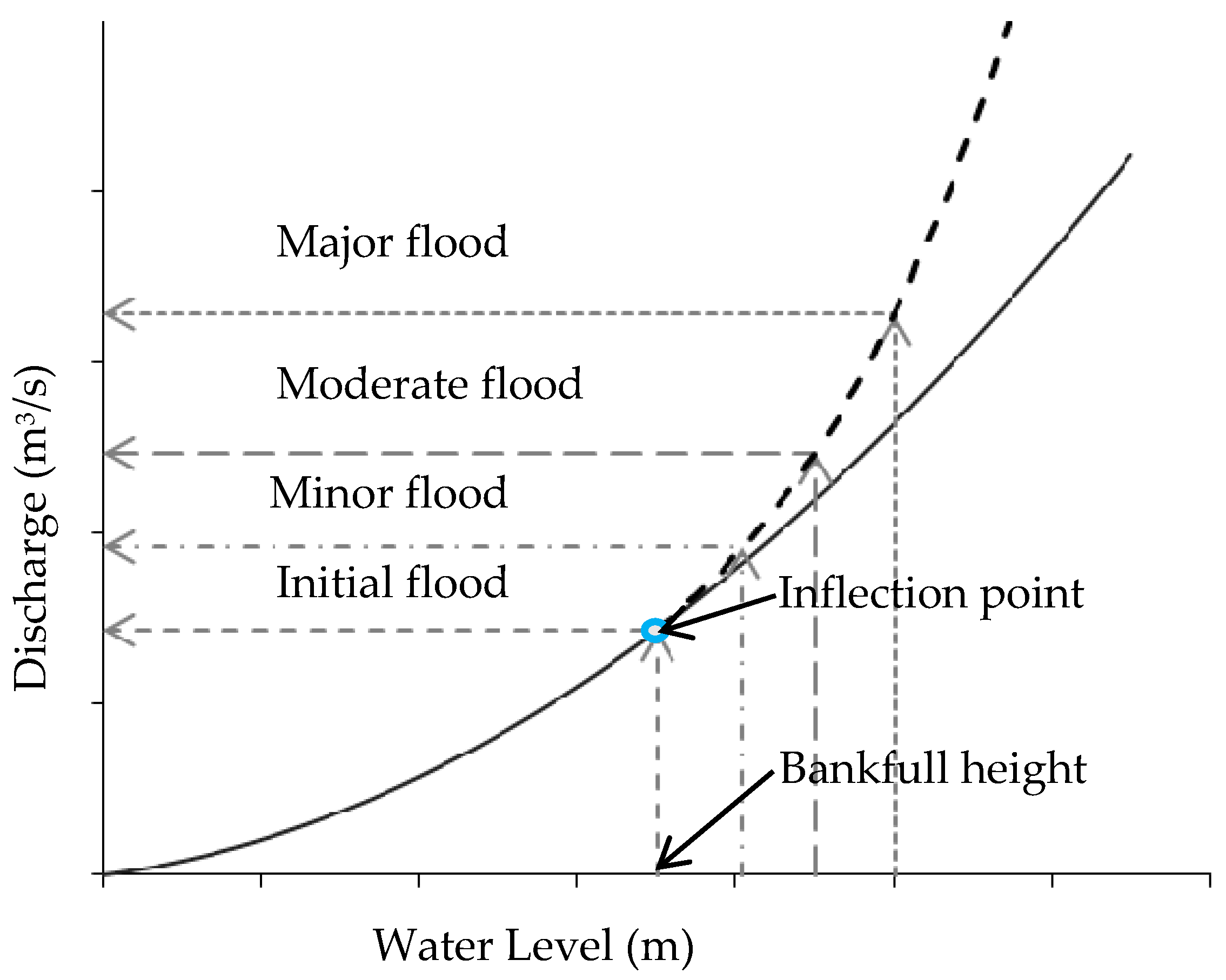
In addition to the AM and POT flood series, the BF flood series were derived to overcome some of the uncertainties in deriving a POT series. While the AM series excludes some historical floods, the POT series may produce some unrealistic floods depending on the selection of the flood threshold value in the analysis. One way to reduce this uncertainty is to use an actual flood discharge as the POT value corresponds to a specific flood category as shown in Figure 2. As our interest is to quantify small magnitude floods, the BF series was produced by taking account of all floods equal to or greater than the initial flood category and the flood series were extracted by using the initial flood discharge as the flow threshold. The initial flood discharge corresponds to the first occurrence of over bank flow and is conceptually slightly greater than the BF discharge (Figure 2). The BF flood series were identified from the stage-discharge relationship and river bank elevation at the gauging site. Often an inflection point on the stage-discharge relationship indicates the BF discharge. In an earlier study, Wallace et al. [30] derived initial flood levels for all GBR catchments based on historical flood data and river bank heights. This study used the flood levels reported in Wallace et al. [30] and gauged water level and discharge data to estimate BF discharge. An average discharge value corresponding to initial flood level for the entire data record was used to estimate the flood threshold. Accordingly, the BF flood series were generated for each of the 24 study catchments using the POT approach. Historical flood frequencies were estimated based on number of floods in the BF series and the length of data record.
2.4. Flood Indicators
A total of five flood indicators based on the AM, POT and BF series were selected to estimate frequency of small magnitude floods and to compare frequency estimates between flood series (Table 1). This approach is consistent with previous studies (e.g., [13,17,30]). While AM and POT indicators are commonly used for flood frequency, BF discharge is specific to this study and is introduced to construct actual flood series.
2.5. Variability Analysis
The inter-annual variability of flood magnitude across the GBR lagoon catchments was estimated using the commonly used Flash Flood Magnitude Index (FFMI). The FFMI is one of several measures used to identify variability in flood magnitude within and between years [13]. In the past, the FFMI has been used to characterise flood variability in Australian rivers [32]. The FFMI is calculated as the standard deviation of the logarithm of AM flood series as follows:
where Qm is the mean of the AM flood series, N is the number of floods. One characteristic of this measure is that low magnitude floods strongly influence this index [32] and the ecological significance of low magnitude floods is high [4]. This characteristic is particularly important for the GBR lagoon catchments where many rivers are ephemeral or experience multi-year periods of low flow condition.
2.6. Frequency Analysis
Flood data are examined within a magnitude–frequency framework which requires the estimate of the average recurrence interval for each flood. The recurrence interval (Tr) of a flood in a series is the average time interval which the given discharge will be equaled or exceeded once. Discharge data were ranked in descending order and an average recurrence interval was calculated using the Gringorten plotting position formula [33] defined as:
where n is the number of years of data and m is the sample rank based on a descending flood series. A flood with a recurrence interval of Tr years is denoted as QT.
Based on observed flow data and the magnitude–frequency relationship, flood frequency models were developed using different probability models. Both in Australia and North America, the Pearson Type 3 distribution fitted to the log-transformed flood series, referred to as the Log Pearson 3 (LP3) distribution, has traditionally been recommended for flood frequency modelling [34]. In a recent study based on a large set of Australian flood data, Rahman et al. [35] recommended comparing LP3, Generalised Extreme Value (GEV), and Generalised Pareto (GPA) before selecting a distribution. A common way of testing a best fit probability distribution is to compare an L-moment ratio diagram [36]. Based on recommendations from previous studies (e.g., [35,37]), five frequency models, GEV, GPA, LP3, Log Normal (LN) and Weibull (WB) were tested using L-moment ratio diagrams. Frequencies of small floods ranging from 1 to 20 years were estimated using the best fit models. Flood frequency estimates based on the AM and POT series were evaluated compared to the BF series. The flood frequency analysis was conducted using an extreme value analysis package in R [38].
3. Results
3.1. Historical Floods
The rivers in the GBR lagoon catchments experience a range of flood and flow regimes, having on average two to three floods in a year to less than one flood in some areas (Table 2). Catchments in the northern part of the GBR lagoon experience more than one flood per year (Site ID 102 to 117). For those catchments in close proximity to the coast, tropical cyclones commonly produce high-magnitude, short-duration floods. Compared to the wet tropical region (Site ID 108 to 116), catchments in the relatively dry climate (Site ID 120 to 138) experience less frequent floods (on average less than one flood in a year). Catchments in the wet tropical region are subject to frequent flooding because of frequent and intense rainfall (mean annual rainfall ~2000 mm) and high antecedent soil water conditions [39].
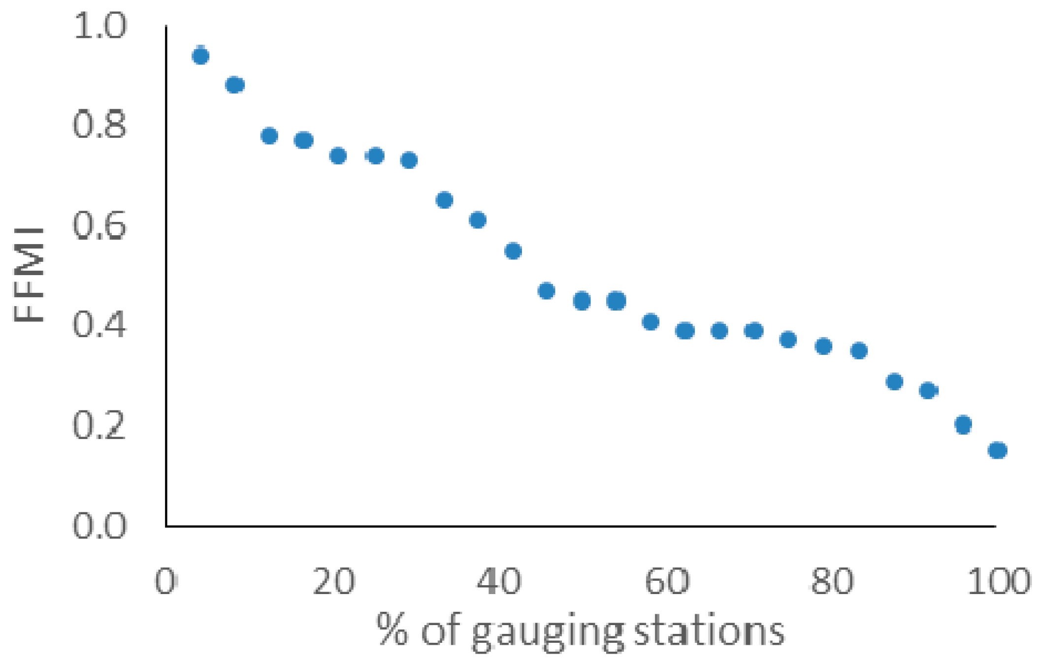
Flood variability, as measured by FFMI, varies considerably across the GBR catchments (Table 2). The FFMI ranges from 0.15 (Tully) to 0.91 (Kolan) and 50% of the gauges recorded a FFMI of 0.45 or more (Figure 3). The GBR catchment observed a very similar mean FFMI to other Australian and South African rivers, however, the value is considerably larger compared to the rivers from the rest of the world (Table 3). Relatively small FFMI values are found for the catchments that experience frequent flooding (Site ID 108 to 116). Flood variability increases southwards.
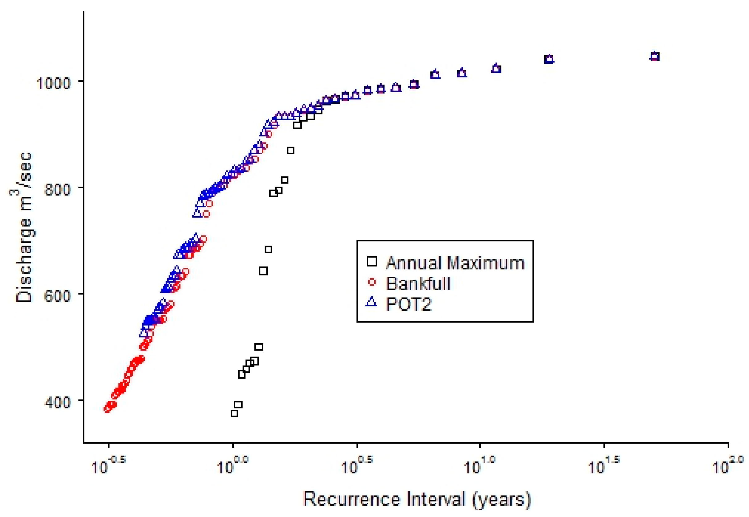
Figure 4 represents a typical example of comparing estimated flood magnitudes of different recurrence intervals for the AM, POT and BF series. For this example, differences in flood magnitude between the different methods occur mostly for the floods of 3 years or less recurrence intervals. Results clearly indicate that the AM series underestimates the low magnitude flood frequency for all catchments irrespective of catchment properties. However, the scale of underestimation depends on flood flow regimes of a catchment. As expected, the POT series produce better estimates for low magnitude floods because the series takes into account all floods above the threshold.
While the POT method produces better estimates of flood magnitudes for small magnitude floods, frequency estimates for different series could differ between two or more POT series. Figure 5 shows examples of estimated flood magnitudes using 3 thresholds (POT1, POT2 and POT2.5) for two climatically different river catchments. In both cases, estimates of flood magnitude for different recurrence intervals differ based on the POT value. However, the difference is relatively small for the wet tropical catchment (Site ID 113) where floods are frequent (Figure 5a) compared to the dry tropical catchments where floods are less frequent (Figure 5b).
It is interesting to note that lowering the POT threshold does not necessarily increase the flood frequency even though it produces more floods; in fact, a low flood threshold decreases the frequency (Figure 5). Results suggest that a low threshold value may merge two or more large magnitude floods into a single one, and consequently, reduce frequency of flooding in many instances (Table 4). It is also noted that a low threshold produces some unrealistic floods at the bottom end of the frequency curve (i.e., small magnitude, Figure 5b).
Figure 6 compares flood magnitudes for the AM, POT and BF series at wet tropical (Site ID 114) and dry tropical (Site ID 119) catchments. As seen in the previous sections, in both cases the AM series underestimates discharges for lower magnitude floods (average recurrence interval (ARI) of less than 10 years). In this particular example, both the AM and POT series underestimated the frequencies compared to the BF series. It is interesting to note that the AM and POT series produced some unrealistic floods at small recurrence intervals (i.e., discharge value less than BF, Site ID 119). Results confirm that discharge is underestimated particularly in catchments that experience less frequent floods (Site ID 119) compared to those that experience frequent floods (Site ID 114).
3.2. Frequency Distribution Models
Figure 7 shows L-moment ratio diagrams for the AM and POT flood series for the five commonly used probability models (GEV, GPA, LN, LP3, WB). Of the five models examined, the GPA model fits better to the data obtained from both the AM and POT flood series. Results are consistent with the findings by Rustomji et al. [13] for the catchments in the east coast of Australia. Consequently, the GPA model was used in the subsequent flood frequency analysis.
3.3. Frequency of Small Floods
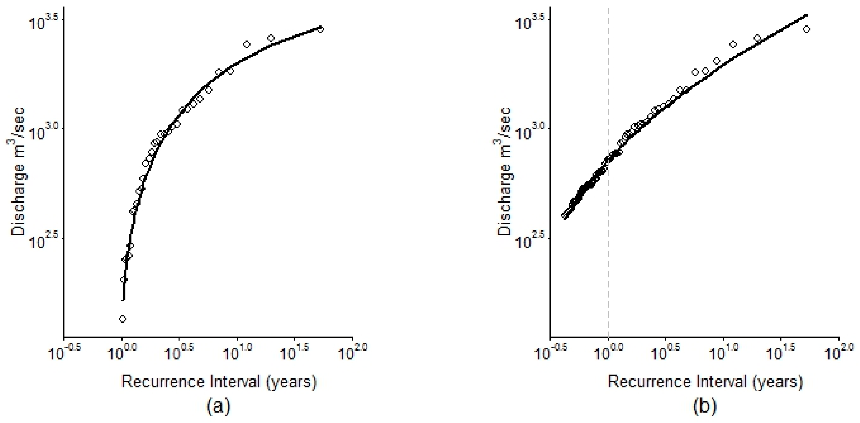
The probability distribution model (GPA) fitted to both the AM and POT flood series provides a fairly good fit to the observed data. Figure 8 shows an example of fitted flood frequency distributions against the observed data for the AM and POT2 series for the Gauge 113,006 on the Tully River (Site ID 113 in Table 1). Results clearly indicate that AM series underestimates frequency of low magnitude floods. However, the scale of underestimation depends on whether the catchment experiences frequent or less frequent floods (Figure 6b). For any catchment, irrespective of its flood flow regime, the AM series underestimates the frequency of small floods.
Using the fitted GPA model, flood magnitudes for 1, 2, 3, 5, 10 and 20 year recurrence intervals were estimated based on AM and POT series (Table 5). In most cases, flood magnitude is higher for the POT series compared to the AM series for any recurrence interval between 1 and 10 years. However, the difference is relatively larger for frequent floods (e.g., 1 and 2 years interval).
Table 6 presents the ratio of estimated flood discharge for the AM series to that of the BF series with selected recurrence intervals. Smaller ratios were obtained for more frequent floods, indicating a larger difference in the flood magnitudes. For floods with ten year or more recurrence intervals, the ratios are close to one; that is, differences in flood magnitudes produced from either method is minimal. For the most frequent flood the ratio is the smallest, which indicates a difference in flood magnitude is the largest. For recurrence intervals of 10 years or more, estimates from both methods are nearly the same (i.e., no difference in flood frequency). Results show that the selection of a frequency distribution model is less sensitive to estimates of flood magnitude.
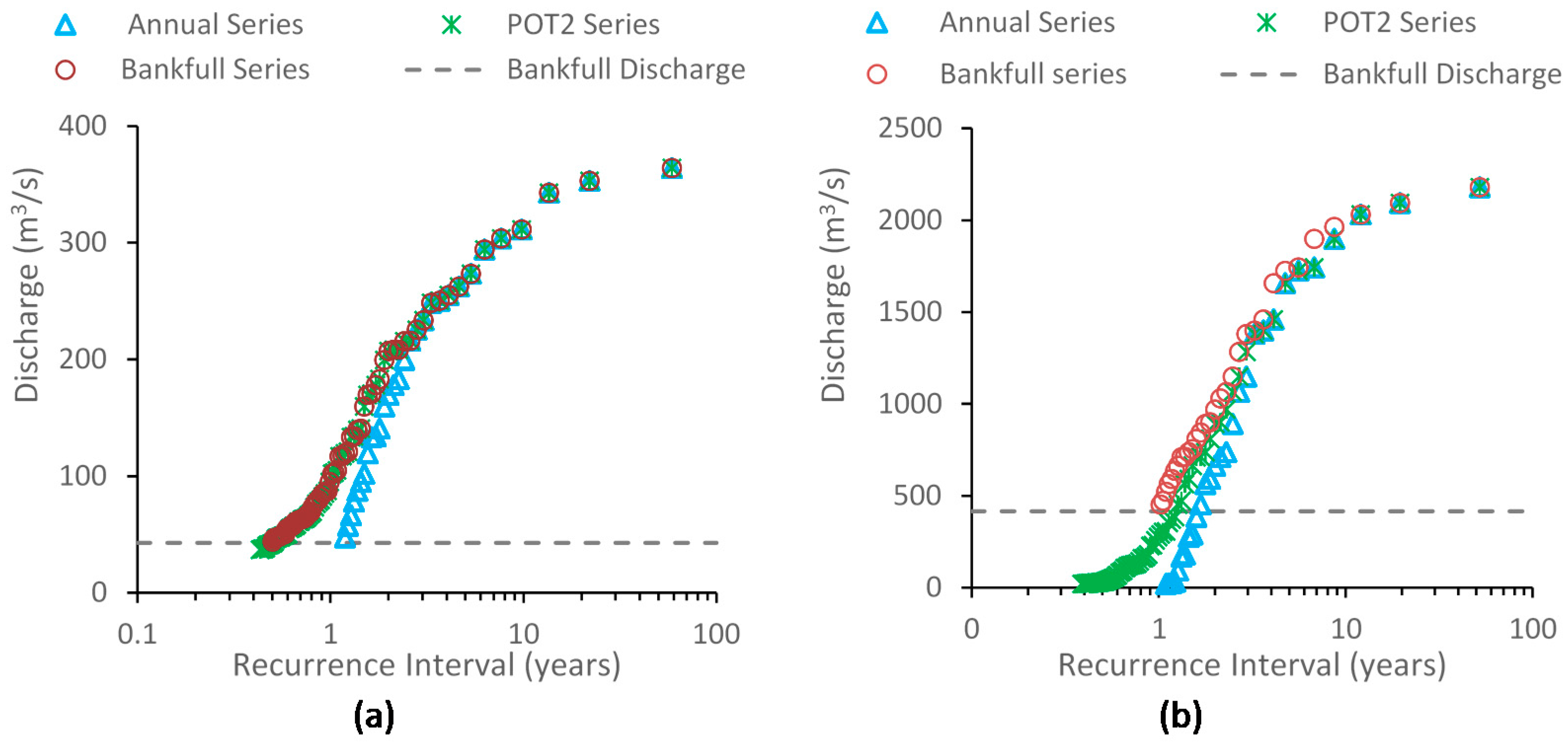
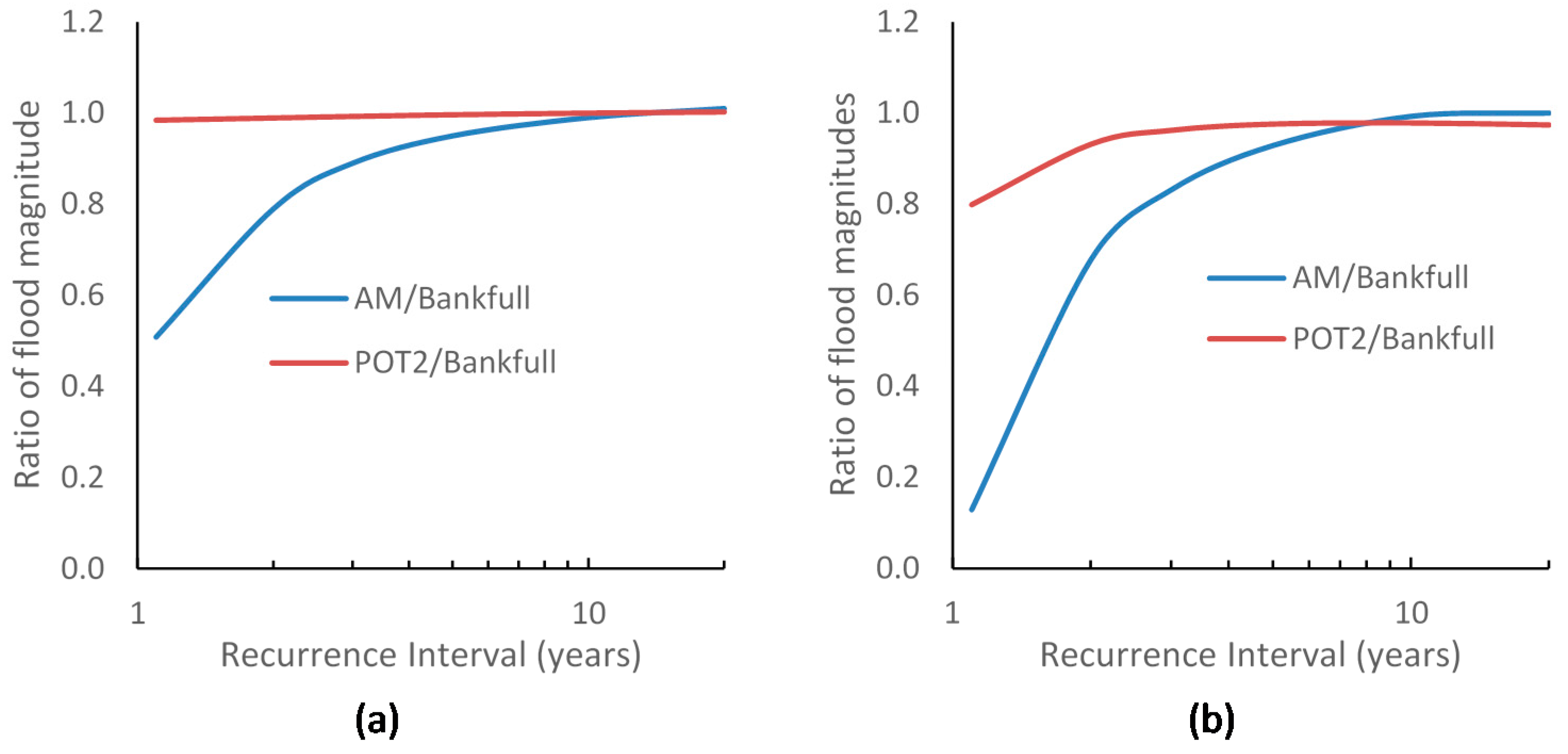
Results show that both the AM and POT series underestimate flood magnitude compared to the BF series for a recurrence interval of less than 10 years. However, the difference is relatively smaller for the POT series compared to the AM series. It can be seen that the difference in estimates of flood magnitude between the AM and BF series is relatively small for a wet tropical catchment (Figure 9a) compared to a dry tropical catchment (Figure 9b). While the POT flood series produces a similar recurrence interval compared to the BF floods for a wet tropical catchment, predictions are less accurate for a dry tropical catchment (Figure 9b).
3.4. Monthly Flood Frequency
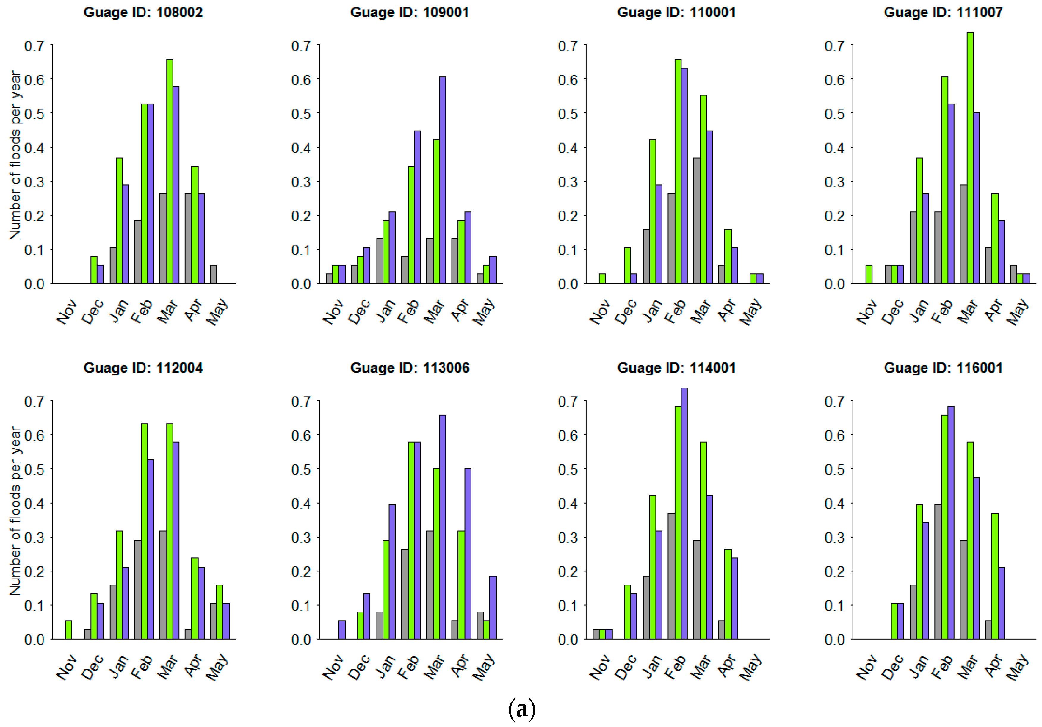
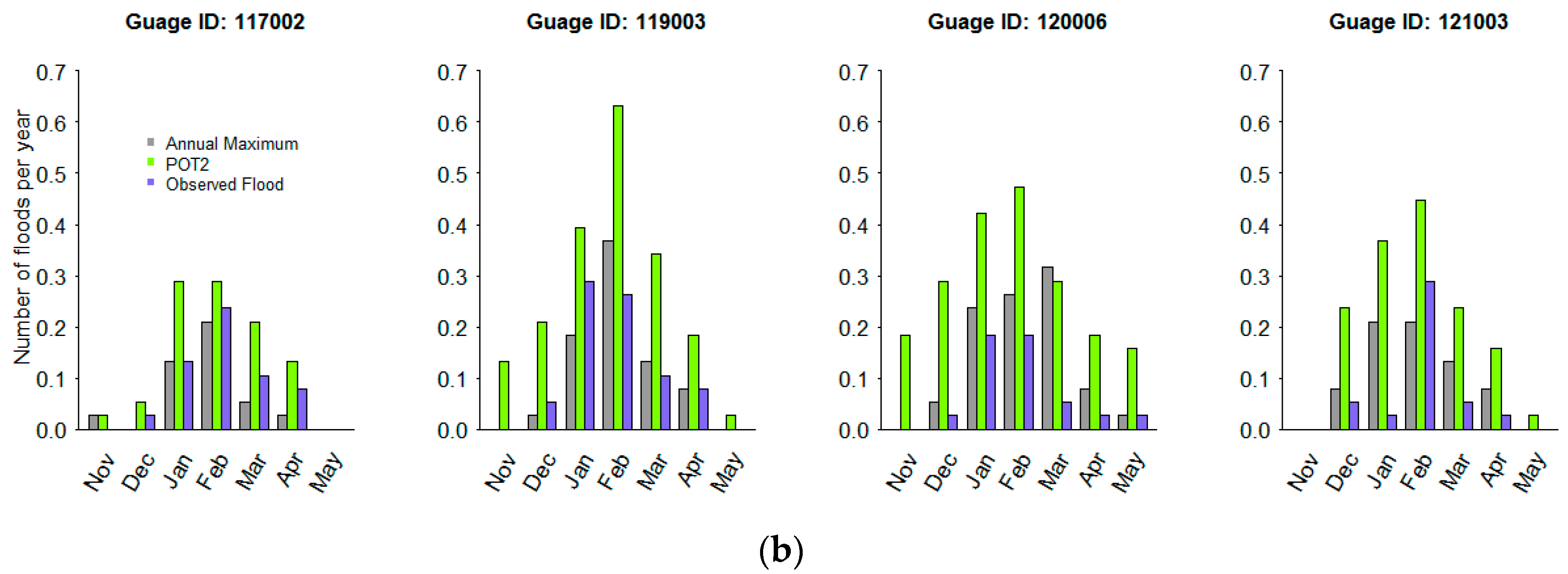
Selection of a flood series influences the frequency of floods between months. Results show that both the AM and POT series differ from the actual monthly flood frequency (Figure 10). As the AM series excludes many historical floods, it reduces the frequencies at which a flood is designated to occur within months. The partial series overestimates frequencies compared to the BF series at a monthly timestep if a small threshold is used and underestimates monthly frequencies if a large threshold is used. We noticed that the impact of the flood series is different between catchments. For the wet tropical catchments, where floods are frequent, the AM series underestimates the flood frequencies between months. While the partial series better predicts the monthly floods for the wet tropical catchments, it overestimates flood frequency for dry tropical catchments where floods are less frequent.
4. Discussion
Both flood magnitudes and frequencies vary between catchments based on physical (e.g., catchment size) and climatic (e.g., rainfall) conditions. Catchments located in the wet tropical region (Site ID 108 to 116) experience more frequent floods than those located in the southern dry tropical parts (Site ID 120 to 138). The main reason for high flood frequency in the wet tropical region is the high seasonal rainfall and tropical cyclones, as reported in Alexander et al. [29]. The frequency of flood influences the flood variability; in general, catchments experiencing frequent floods show less variability between floods (e.g., Tully and Mossman catchments). Flood variability is generally high for large catchments, primarily due to large variations in flood magnitudes.
Five frequency distribution models were tested for their goodness of fit. Between frequency models, GEV, GPA and LP3 were found to better represent the flood series data for the GBR lagoon catchments. While the GPA model produced a best fit to historical floods (Figure 7), estimates based on GEV and LP3 models are close to estimates produced by the GPA model (Table 6). This suggests that any of these three statistical distribution models are suitable to estimate flood magnitudes for the GBR lagoon catchments. Results are consistent with the studies of Rustomji et al. [13] and Rahman et al. [35]. There are no significant differences in estimates of flood magnitude between the three selected frequency models (GPA, GEV and LP3).
Most differences in frequency estimates were found for the small magnitude floods (e.g., one year recurrence interval). While both series produce similar results for engineering applications (i.e., large floods), these results have important considerations for the methods by which the flood regime of floodplain ecosystems are assessed. The POT series includes more floods than the AM series; therefore the frequency of small to medium floods is higher compared to the AM series. The main advantages of the POT series are that the series excludes insignificant floods and produces more data points, which in turn improves the accuracy of frequency estimates, especially if the data length is short [18]. However, the POT series is less commonly used in flood design studies because of the complexity in identifying independent floods and obviously there is no significant improvement in results compared to the AM series for large floods [16]. Therefore, the AM series serves the purpose for any engineering design (e.g., bridge, culvert, levee bank).
One of the main disadvantages of the POT series is the selection of the threshold value. Without prior knowledge of actual flood flow, it is difficult to identify a realistic flood threshold value. As the threshold selection is an iterative process, one could easily choose any higher or even lower threshold value, but the lower threshold provides some advantages regarding sample size, and the results of statistical tests were considerably better if more data points are added. Historically, the AM series was used because of its greater computational convenience and avoidance of dependence problems.
While previous studies (e.g., [14,16,20,21]) as well this study clearly indicate that the POT series better estimates small magnitude floods compared to the AM series, the POT method is not error free. As the selection of a POT discharge is an iterative process, it can produce fewer or greater numbers of floods compared to historical floods and there are still uncertainties on frequency estimates based on POT series. As seen in the results section, flood frequency estimates are better if the POT discharge is close to actual flood discharge. Therefore, prior knowledge of actual flood discharge is useful for investigating flood frequencies using the POT method.
One of the main findings of this study is that neither the AM nor the POT series can produce frequency of small magnitude floods accurately, although the POT based estimates are better compared to the AM series. The analysis based on actual flood discharge shows that the POT series can underestimate the flood frequency (Figure 9), although the difference between the POT and BF series is relatively small. Similar to the AM series, the POT series also produces insignificant floods if a small flood threshold is used (Figure 6). For example, a low threshold value for the POT method can grossly overestimate monthly frequency of floods (Figure 10). Also, results showed that the difference in frequency estimates between the AM and POT series compared to the BF series differ across the region. For example, for a wet tropical catchment where floods are frequent, the POT series very much mimics the BF series estimates, but for a dry tropical catchment where floods are less frequent, the POT series estimates differ from the BF series. Therefore, a good way of reducing uncertainty in POT method is to identify the BF discharge and use the BF discharge as the flood threshold. However, there are also uncertainties on observed flow data as the discharge is often calculated using a single rating curve for in-bank and overbank flow. More research is needed to produce a better rating curve, especially for overbank flow conditions. This will help in quantifying bankfull discharge using stage-discharge relationship and river bank height.
5. Conclusions
This article presents results from an analysis of low magnitude floods in the Great Barrier Reef lagoon catchments along the north-east coast of Australia. Flood frequency analyses were carried out with the AM and POT series. While both methods produce similar magnitudes for large floods, considerable differences were calculated for small floods ranging from one to five years average recurrence interval. For a mean annual flood (i.e., average recurrence interval of one year), discharge estimates based on the AM series are approximately one third of the magnitude of POT series estimates and the ratio converges to one in between the five to ten year recurrence interval for the majority of the rivers in the GBR lagoon catchments. This study also found that estimates of flood magnitude vary between the probability models, but the difference is small. Results also suggest that there is a difference in flood estimates based on a subjective threshold compared to the actual flood threshold corresponding to the BF discharge. One important finding is that the estimated flood discharge for a particular recurrence interval decreases with decreasing flood threshold, due to the merging of two or more floods at lower thresholds. Also, results showed that the impact of the flood threshold is insignificant for a river catchment experiencing frequent flooding (e.g., Site ID 113), while the difference in flood magnitudes for different POT series is pronounced for a dry tropical river where flooding is less frequent.
These results suggest that the AM series is not suitable for predicting low magnitude floods, especially for floods with an average recurrence interval of five years or less, as it significantly underestimates the magnitude. While this study included only one gauging site in each river catchment, the results of this study are consistent with previous studies for the region and across the world. Findings of this research are significant for future studies on ecology, as many of the ecological aspects are largely influenced by the frequency of floods.
Acknowledgments
The authors wish to thank the Department of Natural Resources and Mines of the Queensland Government for supplying stream flow and catchments attributes data. We thank Cuan Petheram, Catherine Ticehurst, Justin Hughes and Yuan Chen of CSIRO and two anonymous reviewers for their constructive comments on an earlier version of this manuscript.
Author Contributions
Fazlul Karim conceived and designed the research work. Fazlul Karim and Masud Hasan developed the statistical model and performed the analyses. Steve Marvanek performed spatial analysis. All authors contributed in data processing and manuscript writing.
Conflicts of Interest
The authors declare that there are no conflicts of interest.
References
- The National Flood Risk Advisory Group. Flood risk management in Australia, National Flood Risk Advisory Group (NFRAG). Aust. J. Emerg. Manag. 2008, 23, 21–27. [Google Scholar]
- Luo, P.; He, B.; Takara, K.; Xiong, Y.E.; Nover, D.; Duan, W.; Fukushi, K. Historical assessment of Chinese and Japanese flood management policies and implications for managing future floods. Environ. Sci. Policy 2015, 48, 265–277. [Google Scholar] [CrossRef]
- Markus, M.; Demissie, M. Predictability of annual sediment loads based on flood events. J. Hydrol. Eng. 2006, 11, 354–361. [Google Scholar] [CrossRef]
- Junk, W.J.; Bayley, P.B.; Sparks, R.E. The flood pulse concept in river-floodplain systems. Can. Spec. Publ. Fish. Aquat. Sci. 1989, 106, 110–127. [Google Scholar]
- Tockner, K.; Malard, F.; Ward, J.V. An extension of the flood pulse concept. Hydrol. Process. 2000, 14, 2861–2883. [Google Scholar]
- Bunn, S.E.; Arthington, A.H. Basic principles and ecological consequences of altered flow regimes for aquatic biodiversity. Environ. Manag. 2002, 30, 492–507. [Google Scholar] [CrossRef]
- Godfrey, P.C.; Arthington, A.H.; Pearson, R.G.; Karim, F.; Wallace, J. Fish larvae and recruitment patterns in floodplain lagoons of the Australian Wet Tropics. Mar. Freshw. Res. 2016, 68, 964–979. [Google Scholar] [CrossRef]
- Karim, F.; Petheram, C.; Marvanek, S.; Ticehurst, C.; Wallace, J.; Hasan, M. Impact of climate change on floodplain inundation and hydrological connectivity between wetlands and rivers in a tropical river catchment. Hydrol. Process. 2016, 30, 1574–1593. [Google Scholar] [CrossRef]
- Bendix, J. Flood disturbance and the distribution of riparian species diversity. Geogr. Rev. 1997, 87, 468–483. [Google Scholar] [CrossRef]
- Poff, N.L. Ecological response to and management of increased flooding caused by climate change. Philos. Trans. R. Soc. Lond. 2002, 360, 1497–1510. [Google Scholar] [CrossRef] [PubMed]
- Arthington, A.H.; Godfrey, P.C.; Pearson, R.G.; Karim, F.; Wallace, J. Biodiversity values of remnant freshwater floodplain lagoons in agricultural catchments: Evidence for fish of the wet tropics bioregion, northern Australia. Aquat. Conserv. Mar. Freshw. Ecosyst. 2014, 25, 336–352. [Google Scholar] [CrossRef]
- Hu, G.-M.; Ding, R.-X.; Li, Y.-B.; Shan, J.-F.; Yu, X.-T.; Feng, W. Role of flood discharge in shaping stream geometry: Analysis of a small modern stream in the Uinta Basin, USA. J. Palaeogeogr. 2017, 6, 84–95. [Google Scholar] [CrossRef]
- Rustomji, P.; Bennett, N.; Chiew, F. Flood variability east of Australia’s Great Dividing Range. J. Hydrol. 2009, 374, 196–208. [Google Scholar] [CrossRef]
- Keast, D.; Ellison, J. Magnitude frequency analysis of small floods using the annual and partial series. Water 2013, 5, 1816–1829. [Google Scholar] [CrossRef]
- Zaman, M.A.; Rahman, A.; Haddad, K. Regional flood frequency analysis in arid regions: A case study for Australia. J. Hydrol. 2012, 475, 74–83. [Google Scholar] [CrossRef]
- Petrow, T.; Merz, B. Trends in flood magnitude, frequency and seasonality in Germany in the period 1951–2002. J. Hydrol. 2009, 371, 129–141. [Google Scholar] [CrossRef]
- Bacova-Mitkova, V.; Onderka, M. Analysis of extreme hydrological events on the Danube using the peak over threshold method. J. Hydrol. Hydromech. 2010, 58, 88–101. [Google Scholar] [CrossRef]
- Armstrong, W.H.; Collins, M.J.; Snyder, N.P. Increased frequency of low-magnitude floods in New England. J. Am. Water Resour. Assoc. 2012, 48, 306–320. [Google Scholar] [CrossRef]
- Ball, J.; Babister, M.; Nathan, R.; Weeks, W.; Weinmann, E.; Retallick, M.; Testoni, I. Australian Rainfall and Runoff: A Guide to Flood Estimation; Commonwealth of Australia: Canberra, Australia, 2016. [Google Scholar]
- Adamowski, K.; Liang, G.-C.; Patry, G.G. Annual maxima and partial duration Food series analysis by parametric and non-parametric methods. Hydrol. Process. 1998, 12, 1685–1699. [Google Scholar] [CrossRef]
- Bezak, N.; Brilly, M.; Šraj, M. Comparison between the peaks-over-threshold method and the annual maximum method for flood frequency analysis. Hydrol. Sci. J. 2014, 59, 959–977. [Google Scholar] [CrossRef]
- Beguería, S. Uncertainties in partial duration series modelling of extremes related to the choice of the threshold value. J. Hydrol. 2005, 303, 215–230. [Google Scholar] [CrossRef]
- Lang, M.; Ouarda, T.B.; Bobee, B. Towards operational guidelines for over-threshold modeling. J. Hydrol. 1999, 225, 103–117. [Google Scholar] [CrossRef]
- Great Barrier Reef Marine Park Authority. Population and Major Land Use in the Great Barrier Reef Catchment Area: Spatial and Temporal Trends; Great Barrier Reef Marine Park Authority (GBRMPA): Townsville, Australia, 2001; p. 79.
- Karim, F.; Kinsey-Henderson, A.; Wallace, J.; Godfrey, P.; Arthington, A.H.; Pearson, R.G. Modelling hydrological connectivity of tropical floodplain wetlands via a combined natural and artificial stream network. Hydrol. Process. 2014, 28, 5696–5710. [Google Scholar] [CrossRef]
- Pearson, R.G.; Godfrey, P.C.; Arthington, A.H.; Wallace, J.; Karim, F.; Ellison, M. Biophysical status of remnant freshwater floodplain lagoons in the great barrier reef catchment: A challenge for assessment and monitoring. Mar. Freshw. Res. 2013, 64, 208. [Google Scholar] [CrossRef]
- Hopkins, L.C.; Holland, G.J. Australian heavy-rain days and associated east coast cyclones: 1958–92. J. Clim. 1997, 10, 621–635. [Google Scholar] [CrossRef]
- McBride, J.L.; Nicholls, N. Seasonal relationships between Australian rainfall and the southern oscillation. Mon. Weather Rev. 1983, 111, 1998–2004. [Google Scholar] [CrossRef]
- Alexander, J.; Fielding, C.R.; Pocock, G.D. Flood behaviour of the Burdekin river, tropical north Queensland, Australia. Special Publications. Geol. Soc. Lond. 1999, 163, 27–40. [Google Scholar] [CrossRef]
- Wallace, J.; Karim, F.; Wilkinson, S. Assessing the potential underestimation of sediment and nutrient loads to the Great Barrier Reef lagoon during floods. Mar. Pollut. Bull. 2012, 65, 194–202. [Google Scholar] [CrossRef] [PubMed]
- Rustomji, P. A Statistical Analysis of Flood Hydrology and Bankfull Discharge for the Daly River Catchment, Northern Territory, Australia; Commonwealth Scientific and Industrial Research Organisation: Canberra, Australia, 2009; p. 73. [Google Scholar]
- Erskine, W.D. Erosion and deposition produced by a catastrophic flood on the genoa river, Victoria. Aust. J. Soil Water Conserv. 1993, 6, 35–43. [Google Scholar]
- Gringorten, I.I. A plotting rule for extreme probability paper Journal of Geophysical Research. Oceans 1963, 68, 813–814. [Google Scholar] [CrossRef]
- Pilgrim, D.H.; Doran, D.G. Flood frequency analysis. In Australian Rainfall and Runoff: A Guide to Flood Estimation; Pilgrim, D.H., Ed.; Academic Press: Sydney, Australia, 1987; pp. 197–236. [Google Scholar]
- Rahman, A.S.; Rahman, A.; Zaman, M.A.; Haddad, K.; Ahsan, A.; Imteaz, M. A study on selection of probability distributions for at-site flood frequency analysis in Australia. Nat. Hazards 2013, 69, 1803–1813. [Google Scholar] [CrossRef]
- Vogel, R.M.; Fennessey, N.M. L moment diagrams should replace product moment diagrams. Water Resour. Res. 1993, 29, 1745–1752. [Google Scholar] [CrossRef]
- Vogel, R.M.; McMahon, T.A.; Chiew, F.H.S. Floodflow frequency model selection in Australia. J. Hydrol. 1993, 146, 421–449. [Google Scholar] [CrossRef]
- Gilleland, E.; Katz, R.W. Extremes 2.0: An extreme value analysis package. J. Stat. Softw. 2016, 72, 1–39. [Google Scholar] [CrossRef]
- Wallace, J.; Stewart, L.; Hawdon, A.; Keen, R.; Karim, F.; Kemei, J. Flood water quality and marine sediment and nutrient loads from the Tully and Murray catchments in north Queensland, Australia. Mar. Freshw. Res. 2009, 60, 1123–1131. [Google Scholar] [CrossRef]
- McMahon, T.A.; Finlayson, B.L.; Haines, A.T.; Srikanthan, R. Global Runoff: Continental Comparisons of Annual Flows and Peak Discharges; Catena Verlag: Cremlingen-Destedt, Germany, 1992. [Google Scholar]
Figure 1.
Catchments of the Great Barrier Reef (GBR) lagoon showing major rivers and stream gauges. The numbers on the map represent catchment identification and the catchment name under each identification number is presented in the results section.
Figure 1.
Catchments of the Great Barrier Reef (GBR) lagoon showing major rivers and stream gauges. The numbers on the map represent catchment identification and the catchment name under each identification number is presented in the results section.
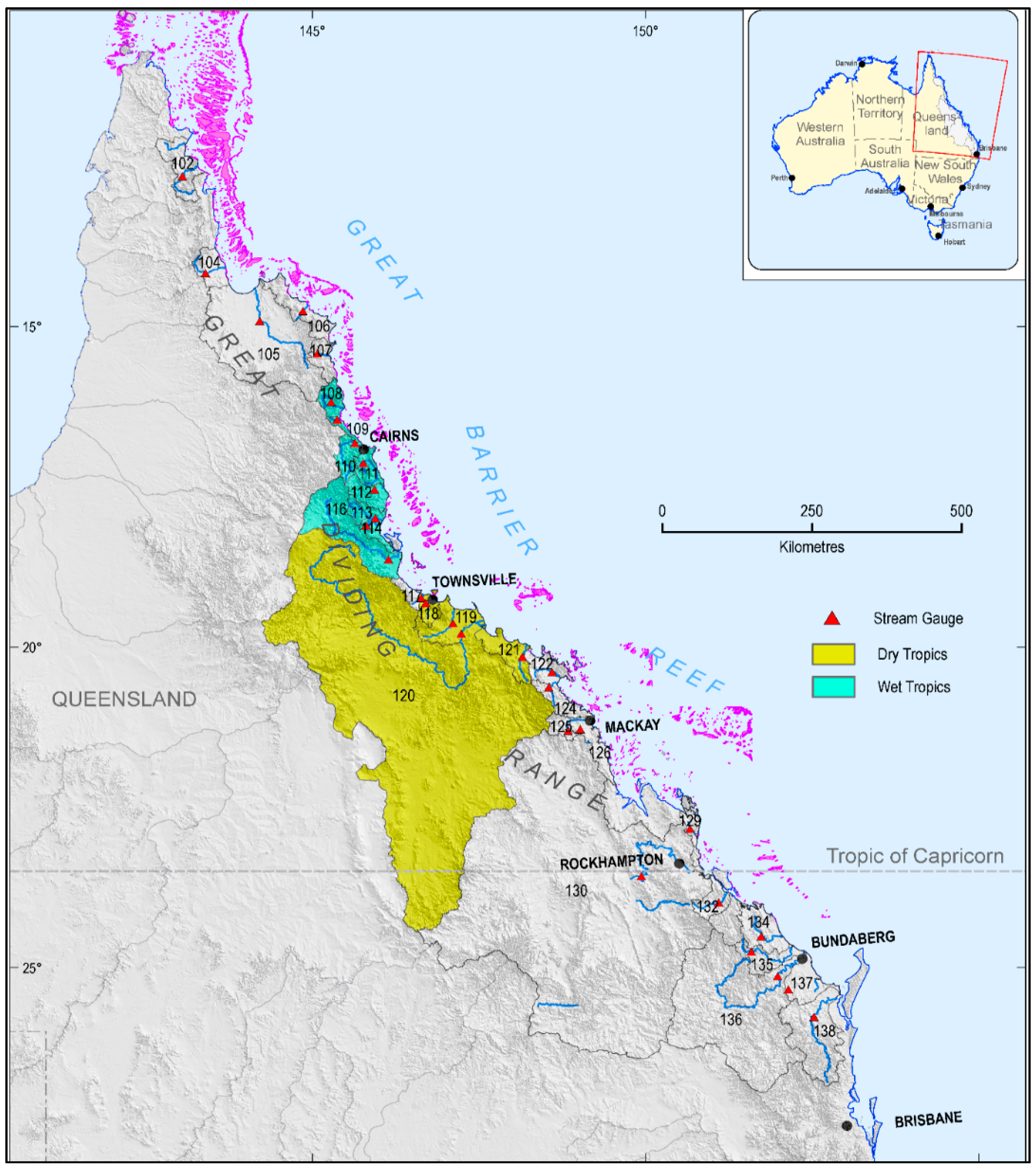
Figure 2.
A streamflow rating curve showing flood categories for a typical river. An initial flood is defined as the bankfull (BF) discharge when the river starts flowing over bank.
Figure 2.
A streamflow rating curve showing flood categories for a typical river. An initial flood is defined as the bankfull (BF) discharge when the river starts flowing over bank.

Figure 3.
FFMI for the GBR lagoon catchments.

Figure 4.
Example of magnitude and frequency estimates using the annual maximum (AM), peak over threshold (POT) and BF flood series for the Tully River (Site ID 113). The POT series includes many more floods than the AM series and thus frequent floods have a larger magnitude.
Figure 4.
Example of magnitude and frequency estimates using the annual maximum (AM), peak over threshold (POT) and BF flood series for the Tully River (Site ID 113). The POT series includes many more floods than the AM series and thus frequent floods have a larger magnitude.

Figure 5.
Comparison of flood magnitude under a given recurrence interval for three POT series for (a) a wet tropical catchment (Site ID 113) and (b) a dry tropical catchment (Site ID 119).
Figure 5.
Comparison of flood magnitude under a given recurrence interval for three POT series for (a) a wet tropical catchment (Site ID 113) and (b) a dry tropical catchment (Site ID 119).

Figure 6.
Comparison of flood magnitudes between the AM, POT and BF series for different recurrence intervals for: (a) a wet tropical catchment (Site ID 114); and (b) a dry tropical catchment (Site ID 119).
Figure 6.
Comparison of flood magnitudes between the AM, POT and BF series for different recurrence intervals for: (a) a wet tropical catchment (Site ID 114); and (b) a dry tropical catchment (Site ID 119).

Figure 7.
L-moment ratio diagrams for (a) AM series (left) and (b) POT flood series (right) for the river catchments in the GBR catchment in Australia.
Figure 7.
L-moment ratio diagrams for (a) AM series (left) and (b) POT flood series (right) for the river catchments in the GBR catchment in Australia.
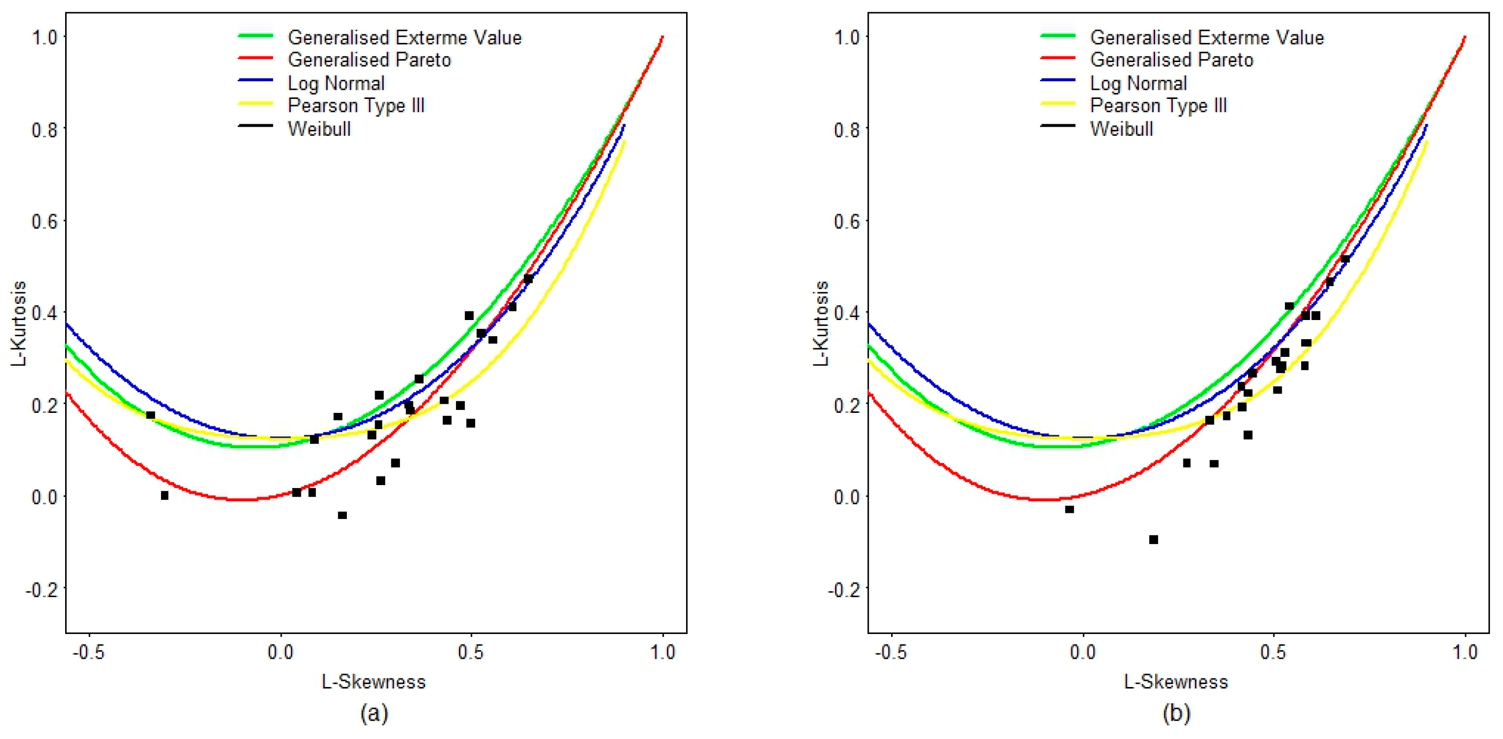
Figure 8.
Comparison between observed flood data and the fitted Generalised Pareto (GPA) distribution (solid line) for the Tully catchment in north Queensland (Site ID 113006, Table 1) for (a) annual flood series; (b) peak over threshold (POT2) flood series.
Figure 8.
Comparison between observed flood data and the fitted Generalised Pareto (GPA) distribution (solid line) for the Tully catchment in north Queensland (Site ID 113006, Table 1) for (a) annual flood series; (b) peak over threshold (POT2) flood series.

Figure 9.
Comparison of recurrence interval and flood magnitude between the AM, partial and BF series for (a) a wet-tropical river (Site ID 114); and (b) a dry-tropical river (Site ID 119).
Figure 9.
Comparison of recurrence interval and flood magnitude between the AM, partial and BF series for (a) a wet-tropical river (Site ID 114); and (b) a dry-tropical river (Site ID 119).

Figure 10.
Monthly flood frequency for the AM and POT series compared to the BF series for (a) wet-tropical and (b) dry-tropical catchments.
Figure 10.
Monthly flood frequency for the AM and POT series compared to the BF series for (a) wet-tropical and (b) dry-tropical catchments.


Table 1.
List of flood indicators used for frequency analysis for all gauges.
| Indicator | Abbreviation | Description |
|---|---|---|
| Annual maximum streamflow (m3/s) | AMAXF | Maximum of daily flow in a water year (July–June) |
| Peak over threshold flow for one flood per year (m3/s) | POT1F | Discharge magnitude that produces on average one flood per year |
| Peak over threshold flow for two floods per year (m3/s) | POT2F | Discharge magnitude that produces on average two floods per year |
| Peak over threshold flow for 2.5 floods per year (m3/s) | POT2.5F | Discharge magnitude that produces on average 2.5 floods per year |
| Bankfull discharge (m3/s) | BF | Discharge magnitude that initiates a flood |
Table 2.
Frequencies of historical floods and flash flood magnitude index (FFMI) for the GBR catchments.
Table 2.
Frequencies of historical floods and flash flood magnitude index (FFMI) for the GBR catchments.
| Site ID | Gauge | River | Catchment Area (km2) | Data Length (Years) | Bankfull Level (m) | Bankfull Discharge (m3/s) | Historical Floods (per Year) | FFMI |
|---|---|---|---|---|---|---|---|---|
| 102 | 102102 | Pascoe | 4197 | 32 | 8.00 | 514 | 1.72 | 0.36 |
| 104 | 104001 | Stewart | 2679 | 29 | 4.10 | 102 | 1.62 | 0.39 |
| 105 | 105107 | Normanby | 24,624 | 10 | 5.30 | 621 | 1.56 | 0.20 |
| 106 | 106002 | Jeannie | 3577 | 17 | 6.20 | 84 | 1.18 | 0.39 |
| 107 | 107001 | Endeavour | 2065 | 30 | 3.40 | 55 | 1.80 | 0.45 |
| 108 | 108002 | Daintree | 1893 | 33 | 5.80 | 282 | 1.97 | 0.35 |
| 109 | 109001 | Mossman | 533 | 22 | 3.20 | 47 | 3.05 | 0.27 |
| 110 | 110001 | Barron | 2135 | 32 | 3.90 | 251 | 1.81 | 0.45 |
| 111 | 111007 | Mulgrave | 1993 | 35 | 4.40 | 275 | 1.71 | 0.37 |
| 112 | 112004 | Johnstone | 2250 | 35 | 3.80 | 419 | 1.89 | 0.29 |
| 113 | 113006 | Tully | 1590 | 30 | 5.40 | 378 | 3.23 | 0.15 |
| 114 | 114001 | Murray | 1042 | 35 | 5.40 | 43 | 2.03 | 0.35 |
| 116 | 116001 | Herbert | 9742 | 35 | 6.40 | 765 | 2.03 | 0.37 |
| 117 | 117002 | Black | 1046 | 18 | 1.50 | 110 | 1.28 | 0.39 |
| 119 | 119003 | Haughton | 4353 | 31 | 4.10 | 417 | 1.00 | 0.78 |
| 120 | 120006 | Burdekin | 130,044 | 35 | 8.50 | 5592 | 0.54 | 0.77 |
| 121 | 121003 | Don | 3538 | 28 | 2.20 | 71 | 0.64 | 0.61 |
| 129 | 129001 | Waterpark | 1629 | 35 | 4.00 | 74 | 0.63 | 0.74 |
| 130 | 130003 | Fitzroy | 142,460 | 30 | 13.60 | 3180 | 0.47 | 0.65 |
| 132 | 132001 | Calliope | 2175 | 34 | 8.40 | 250 | 0.82 | 0.88 |
| 134 | 134001 | Baffle | 3970 | 32 | 9.00 | 299 | 0.81 | 0.74 |
| 135 | 135002 | Kolan | 2904 | 26 | 3.40 | 67 | 0.96 | 0.91 |
| 136 | 136001 | Burnett | 33,274 | 18 | 9.40 | 1552 | 0.33 | 0.65 |
| 138 | 138014 | Mary | 9450 | 33 | 5.10 | 1149 | 0.73 | 0.73 |
Table 3.
Flood variability indices for the GBR lagoon catchments compared to the rest of Australia and world rivers.
Table 3.
Flood variability indices for the GBR lagoon catchments compared to the rest of Australia and world rivers.
| Region | Number of Gauges | Mean FFMI | Reference |
|---|---|---|---|
| World rivers | 931 | 0.28 | McMahon et al. [40] |
| Australian and southern African rivers | 280 | 0.45 | McMahon et al. [40] |
| Rest of the world rivers | 651 | 0.21 | McMahon et al. [40] |
| Hunter Valley, NSW | 24 | 0.65 | Erskine [32] |
| GBR lagoon catchments | 24 | 0.51 | Present study |
| Wet tropical catchments | 8 | 0.35 | Present study |
Table 4.
Number of floods produced by three different POT series compared to BF floods for the selected catchments across the GBR lagoon.
Table 4.
Number of floods produced by three different POT series compared to BF floods for the selected catchments across the GBR lagoon.
| Gauge | Bankfull | Total Floods | Floods above Bankfull | ||||
|---|---|---|---|---|---|---|---|
| Floods | POT1 | POT2 | POT2.5 | POT1 | POT2 | POT2.5 | |
| 102102 | 55 | 32 | 63 | 80 | 32 | 55 | 54 |
| 107001 | 54 | 30 | 60 | 75 | 30 | 53 | 53 |
| 113006 | 97 | 30 | 60 | 75 | 30 | 60 | 75 |
| 121003 | 18 | 28 | 56 | 71 | 15 | 13 | 12 |
| 130003 | 14 | 30 | 60 | 75 | 14 | 13 | 12 |
| 135002 | 25 | 26 | 52 | 65 | 25 | 23 | 15 |
| 138014 | 24 | 33 | 66 | 82 | 24 | 22 | 21 |
Table 5.
Estimated flood discharge (m3/s) for selected recurrence intervals using the AM and POT series for 24 gauging sites across the GBR catchments.
Table 5.
Estimated flood discharge (m3/s) for selected recurrence intervals using the AM and POT series for 24 gauging sites across the GBR catchments.
| Gauge | Flood Series | Average Recurrence Interval (Years) | |||||
|---|---|---|---|---|---|---|---|
| 1 | 2 | 3 | 5 | 10 | 20 | ||
| 102102 | AM | 320 | 784 | 1122 | 1515 | 1993 | 2414 |
| POT | 785 | 1056 | 1279 | 1571 | 1988 | 2429 | |
| 104001 | AM | 80 | 151 | 217 | 312 | 469 | 666 |
| POT | 156 | 190 | 225 | 283 | 395 | 562 | |
| 105107 | AM | 910 | 1801 | 1972 | 2028 | 2041 | 2043 |
| POT | 1048 | 1838 | 1939 | 2034 | 2071 | 2080 | |
| 106002 | AM | 49 | 117 | 173 | 245 | 347 | 454 |
| POT | 127 | 181 | 225 | 283 | 364 | 448 | |
| 107001 | AM | 38 | 98 | 146 | 208 | 291 | 376 |
| POT | 85 | 122 | 156 | 203 | 277 | 363 | |
| 108002 | AM | 262 | 654 | 934 | 1253 | 1630 | 1953 |
| POT | 566 | 805 | 996 | 1237 | 1567 | 1899 | |
| 109001 | AM | 81 | 153 | 206 | 267 | 343 | 409 |
| POT | 134 | 173 | 206 | 251 | 321 | 399 | |
| 110001 | AM | 229 | 628 | 947 | 1351 | 1901 | 2456 |
| POT | 525 | 788 | 1017 | 1332 | 1814 | 2365 | |
| 111007 | AM | 238 | 620 | 843 | 1051 | 1240 | 1359 |
| POT | 511 | 694 | 838 | 1015 | 1251 | 1481 | |
| 112004 | AM | 390 | 841 | 1128 | 1420 | 1717 | 1931 |
| POT | 762 | 964 | 1130 | 1347 | 1655 | 1980 | |
| 113006 | AM | 541 | 907 | 988 | 1018 | 1027 | 1028 |
| POT | 867 | 948 | 982 | 1006 | 1021 | 1027 | |
| 114001 | AM | 52 | 166 | 228 | 281 | 325 | 350 |
| POT | 123 | 193 | 237 | 278 | 319 | 346 | |
| 116001 | AM | 683 | 2649 | 4097 | 5790 | 7874 | 9736 |
| POT | 1662 | 3303 | 4538 | 6013 | 7879 | 9600 | |
| 117002 | AM | 63 | 200 | 280 | 353 | 418 | 459 |
| POT | 158 | 232 | 284 | 340 | 405 | 458 | |
| 119003 | AM | 75 | 693 | 1095 | 1510 | 1943 | 2263 |
| POT | 466 | 954 | 1267 | 1586 | 1915 | 2153 | |
| 120006 | AM | 361 | 3340 | 5628 | 8416 | 12,040 | 15,488 |
| POT | 1087 | 3677 | 5729 | 8311 | 11,805 | 15,291 | |
| 121003 | AM | 13 | 39 | 65 | 109 | 193 | 319 |
| POT | 33 | 57 | 82 | 123 | 201 | 318 | |
| 129001 | AM | 4 | 35 | 63 | 103 | 168 | 246 |
| POT | 40 | 67 | 92 | 126 | 181 | 246 | |
| 130003 | AM | 530 | 2196 | 3655 | 5685 | 8824 | 12,469 |
| POT | 1438 | 3031 | 4412 | 6316 | 9222 | 12,550 | |
| 132001 | AM | 25 | 243 | 433 | 695 | 1095 | 1555 |
| POT | 234 | 429 | 597 | 830 | 1185 | 1592 | |
| 134001 | AM | 49 | 236 | 412 | 676 | 1126 | 1710 |
| POT | 231 | 384 | 531 | 754 | 1146 | 1670 | |
| 135002 | AM | 11 | 81 | 151 | 263 | 471 | 766 |
| POT | 71 | 136 | 201 | 306 | 500 | 777 | |
| 136001 | AM | 80 | 511 | 909 | 1494 | 2463 | 3683 |
| POT | 405 | 927 | 1371 | 1970 | 2861 | 3850 | |
| 138014 | AM | 214 | 865 | 1494 | 2458 | 4151 | 6427 |
| POT | 877 | 1607 | 2287 | 3295 | 4988 | 7151 | |
Table 6.
Ratio of flood magnitudes between AM and BF series for the three best fit frequency models: Generalised Extreme Value (GEV), GPA and Log Pearson 3 (LP3). Data presented here are the average of 24 gauging sites across the study region.
Table 6.
Ratio of flood magnitudes between AM and BF series for the three best fit frequency models: Generalised Extreme Value (GEV), GPA and Log Pearson 3 (LP3). Data presented here are the average of 24 gauging sites across the study region.
| Average Recurrence Interval (Years) | |||||||
|---|---|---|---|---|---|---|---|
| Distribution | Percentiles | 1 | 2 | 3 | 5 | 10 | 20 |
| GEV | 10th | 0.34 | 0.66 | 0.77 | 0.86 | 0.94 | 0.96 |
| 50th | 0.50 | 0.82 | 0.93 | 0.99 | 1.01 | 1.02 | |
| 90th | 0.70 | 0.92 | 0.98 | 1.03 | 1.05 | 1.06 | |
| GPA | 10th | 0.31 | 0.65 | 0.77 | 0.87 | 0.95 | 0.94 |
| 50th | 0.44 | 0.81 | 0.94 | 1.00 | 1.01 | 1.01 | |
| 90th | 0.66 | 0.94 | 1.01 | 1.05 | 1.05 | 1.05 | |
| LP3 | 10th | 0.30 | 0.60 | 0.78 | 0.88 | 0.96 | 0.97 |
| 50th | 0.49 | 0.83 | 0.93 | 0.98 | 1.00 | 1.00 | |
| 90th | 0.70 | 0.93 | 1.01 | 1.02 | 1.02 | 1.02 | |
© 2017 by the authors. Licensee MDPI, Basel, Switzerland. This article is an open access article distributed under the terms and conditions of the Creative Commons Attribution (CC BY) license (http://creativecommons.org/licenses/by/4.0/).
Share and Cite
MDPI and ACS Style
Karim, F.; Hasan, M.; Marvanek, S. Evaluating Annual Maximum and Partial Duration Series for Estimating Frequency of Small Magnitude Floods. Water 2017, 9, 481. https://doi.org/10.3390/w9070481
AMA Style
Karim F, Hasan M, Marvanek S. Evaluating Annual Maximum and Partial Duration Series for Estimating Frequency of Small Magnitude Floods. Water. 2017; 9(7):481. https://doi.org/10.3390/w9070481
Chicago/Turabian StyleKarim, Fazlul, Masud Hasan, and Steve Marvanek. 2017. "Evaluating Annual Maximum and Partial Duration Series for Estimating Frequency of Small Magnitude Floods" Water 9, no. 7: 481. https://doi.org/10.3390/w9070481
Note that from the first issue of 2016, this journal uses article numbers instead of page numbers. See further details here.