Characterization of Terrestrial Discharges into Coastal Waters with Thermal Imagery from a Hierarchical Monitoring Program
by
 , ,
, ,
Claudia Ferrara
1,2, 
Massimiliano Lega
3,
Giannetta Fusco
1,2,
Paul Bishop
4 and
Theodore Endreny
5,*
1
Department of Science and Technologies, University of Naples Parthenope, Centro Direzionale di Napoli, Isola C4, 80143 Napoli, Italy
2
CINFAI, (Consorzio Interuniversitario Nazionale per la Fisica delle Atmosfere e delle Idrosfere), 62029 Tolentino (MC), Italy
3
Department of Engineering, University of Naples Parthenope, Centro Direzionale di Napoli, Isola C4, 80143 Napoli, Italy
4
College of Engineering, University of Rhode Island, 102 Bliss Hall 1 Lippitt Rd, Kingston, RI 02881, USA
5
Department of Environmental Resources Engineering, College of Environmental Science and Forestry, SUNY, 402 Baker Labs, 1 Forestry Drive, Syracuse, NY 13244, USA
*
Author to whom correspondence should be addressed.
Water 2017, 9(7), 500; https://doi.org/10.3390/w9070500
Submission received: 13 April 2017
/
Revised: 27 June 2017
/
Accepted: 6 July 2017
/
Published: 11 July 2017
(This article belongs to the Special Issue The Use of Remote Sensing in Hydrology)
Abstract
:Background: The hierarchical use of remotely-sensed imagery from satellites, and then proximally-sensed imagery from helicopter sand drones, can provide a range of spatial and temporal coverage that supports water quality monitoring of complex pollution scenarios. Methods: The study used hierarchical satellite-, helicopter-, and drone-acquired thermal imagery of coastal plumes ranging from 3 to 300 m, near Naples, Italy, and captured temporally- and spatially-overlapping in situ samples to correlate thermal and water quality parameters in each plume and the seawater. Results: In situ sampling determined that between-plume salinity varied by 37%, chlorophyll-a varied by 356%, dissolved oxygen varied by 81%, and turbidity varied by 232%. The radiometric temperature, Trad, for the plume area of interest had a correlation of 0.81 with salinity, 0.74 with chlorophyll-a, 0.98 with dissolved oxygen, and −0.61 with turbidity. Conclusion: This study established hierarchical use of remote and proximal thermal imagery can provide monitoring of complex coastal areas.
1. Introduction
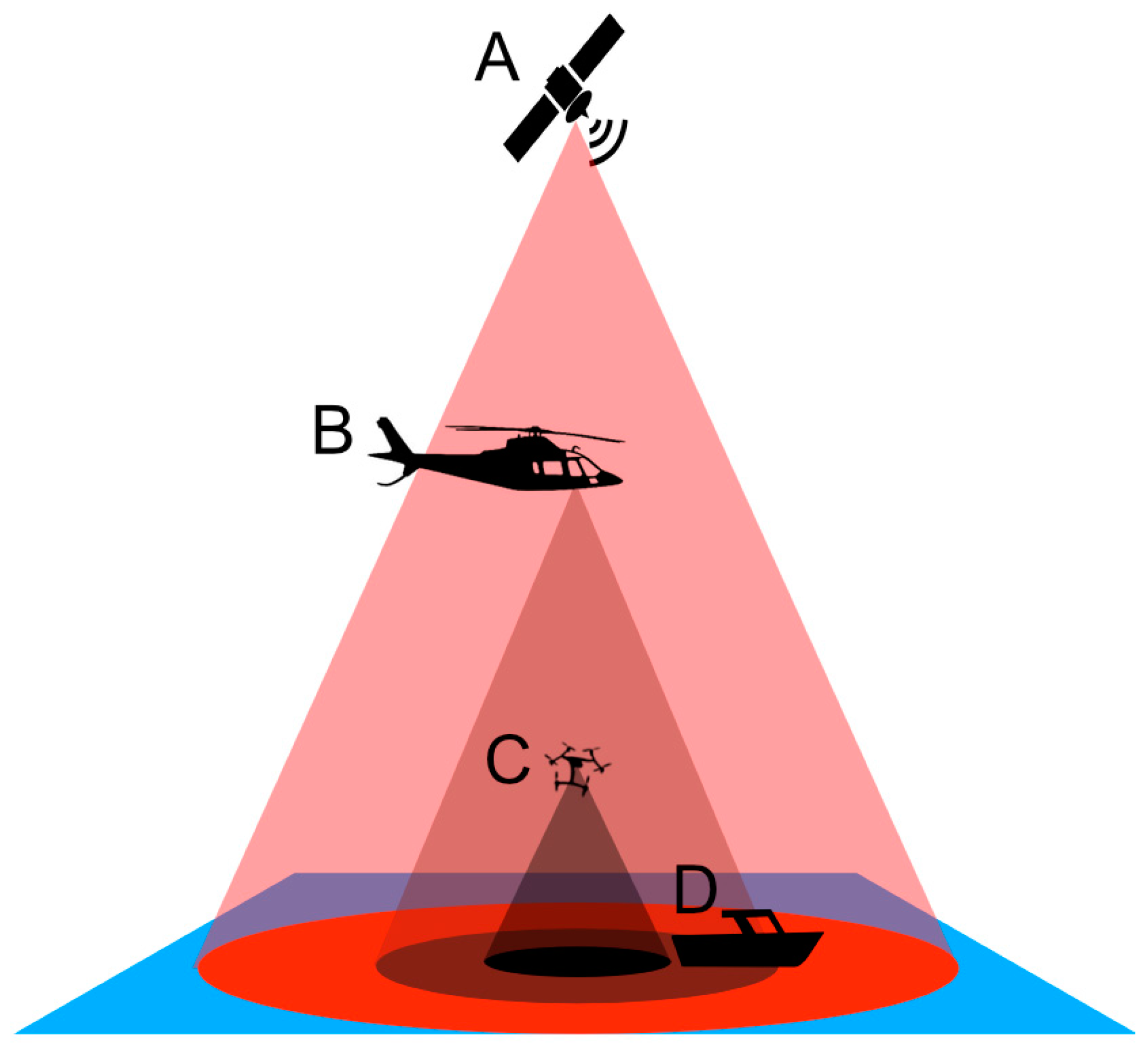
Rapid water quality monitoring of receiving waters is important for the protection and preservation of water and related terrestrial resources. However, in natural systems water quality pollution phenomena can occur across a range of spatial scales, and involve a variety of chemical pollutants, making them difficult and costly to rapidly monitor with in situ retrieval of samples and with a fixed spatial or temporal scale remote sensing approach. Ideally, water quality monitoring of pollutant target areas is spatially and temporally flexible to facilitate the environmental forensics process of characterizing the path of the pollutant between the source and target. To monitor pollution phenomena with extensive spatial or temporal scales, remotely-sensed imagery provides distinct benefits not easily achieved by in situ techniques [1,2] particularly when the pollution interface is affected by dispersion generated by terrestrial inflows to coastal zones [3]. A hierarchical monitoring program is proposed in this manuscript to extend the benefits of water quality monitoring to sites where there are spatial, temporal, financial, and radiometric constraints prohibiting the use of more traditional monitoring with in situ sampling, in situ sensor networks, and remote sensing. A hierarchical monitoring program can use a combination of satellite, helicopter, and drone imagery, as well as in situ sampling (Figure 1), to cover the spatial and temporal scales, and radiometric needs, of the pollution phenomena.
Prior to the emergence of remote sensing hydrology and the evolution of distributed sensor networks, water quality monitoring was traditionally performed using an in situ sample of the water column. In situ samples are either analyzed in real-time by the sampling instrument, such as placing the dissolved oxygen meter into the target water body, or preserved for subsequent analysis in a laboratory. The temporal, spatial, and financial limitations of this approach have encouraged development of remote sensing and in situ sensor-based monitoring. Remote sensing has used airborne and spaceborne hyperspectral and thermal imagery to characterize water quality parameters, establishing relationships with the spectral or temperature signal and the water quality parameter [4]. Hyperspectral sensors detect tens to hundreds of narrow spectral bands throughout the visible, near-infrared, and mid-infrared portions of the electromagnetic spectrum in order to better discriminate between different targets and, as such, can contain the temperature signal [5]. However, hyperspectral sensors generate large volumes of data that create challenges for data storage, manipulation, and water quality analysis.
Nearly all airborne sensors are considered high spatial resolution, ranging between 25 and 0.5 m, and include the Airborne Visible Infrared Imaging Spectrometer manufactured by NASA that provides 17 m resolution, 224 bands, across a 12 km swath width [6]. Spaceborne sensors that are high-resolution (e.g., 20 to 0.5 m) are typically limited to eight bands, and are often operated by commercial firms providing contracted monitoring services [6]. Moderate-resolution sensors include the government-operated Landsat-8 (30 m resolution, 10 bands, 16 day revisit interval) and the Hyperspectral Imager for the Coastal Ocean (100 m resolution, 128 bands, 10 day revisit interval) [6,7,8]. Satellite microwave radiometers used for sea surface temperature water quality studies include the Advanced Microwave Scanning Radiometer-2, with resolution ranging from 5 × 3 km to 62 × 35 km [6].
To summarize the constraints a water quality monitoring program may face with these sensors, at high spatial resolution the monitoring is typically limited to pre-arranged, fee-based campaigns, and, if publicly-available moderate-resolution sensor data are sufficient for the site, the 10 to 16 day revisit interval may become a constraint. As an alternative to radiometric monitoring, finer spatial-and temporal-scale monitoring is available via in situ wireless sensor networks, which relay auto-sampled water quality data to a base station [9]. For some sites, the constraint of these systems include installation, operation, and maintenance costs, their inability to detect pollution extents due to spatial gaps in coverage, and potential interference of the in situ sensor with other activities in those coastal waters.
Thermal infrared imagery, or thermographic data, compared with hyperspectral imagery, are relatively inexpensive and, as such, can allow more resources for increasing spatial and temporal resolution. To capture the peak spectral emission of objects on Earth’s surface, and thereby obtain a suitable signal to noise ratio, the thermographic image should be captured between 9 and 11 μm, which is near the middle of the long-wave infrared electromagnetic spectrum. The thermographic data offer a limited radiometric signal, but contain valuable information on surface properties affecting the energy flux characteristics and dynamics. The radiant energy detected by thermal sensors is a composite of energy emitted by the investigated surface that is transmitted through the atmosphere and energy that is emitted by the atmosphere. While the water-atmosphere coupling complicates interpretation of thermographic data, with proper signal processing researchers can estimate a number of environmental variables important to Earth system science modelling [10].
The thermographic image measures the radiometric temperature, Trad (K), which is related to the thermodynamic, or kinetic, temperature, Tkin (K), is typically measured with a thermometer. The principle of thermographic data analysis is based on the physical phenomenon that all objects at a temperature >0 K emit thermal radiation as a function of the body’s Tkin, and emissivity, ε, which typically ranges depending on properties of the material.
As described by the Stefan-Boltzman law [5], the spectral radiant flux of a black body object, Mb, (W/m2) is:
where σ is the Stefan-Boltzman constant, 5.6697 × 10⁻⁸ W m–2 K–4. As explained by Kirchoff’s Law [5], Equation (1) presumes the black body is a perfect absorber and emitter, with an ε = 1, but otherwise the spectral radiant flux of a real-world object, Mr, is:
where ε < 1, which is the case for most substances [11]. In our work we use the Stefan-Boltzman law to relate the apparent radiant temperature, Trad (K) of the real world object to Mr as:
where Trad is measured by thermal remote sensing. By combining Equations (2) and (3), we can then obtain:
and establish emissivity as the property relating the remotely sensed Trad and the in situ measured Tkin. This same relationship was established by Equation 1.7 in Kuenzer and Dech [12].
In standard processing of multi-pixel infrared thermographic image, it is possible to set only one emissivity value for the whole image. If the observed surface is heterogeneous material (e.g., spatially-varying water chemistry, soil moisture, lithology, or vegetation), the homogenous emissivity will generate erroneous kinetic temperatures for some pixels. However, these discrepancies are diminished when emissivity values approach 1, which is the case for some natural surfaces, such as water. The detection of possible water quality anomalies in coastal waters is made possible by the processing of the multi-pixel thermographic image using a homogeneous emissivity value; for seawater an emissivity value of 0.986 is recommended [13,14]. In monitoring of seawater, when a thermographic pixel captures the radiometric temperature of non-seawater material with the same kinetic temperature but different emissivity than the seawater, the thermographic sensor estimates an erroneous kinetic temperature. In situ measurement of the kinetic temperature in parallel with remote sensing of the radiometric temperature would allow for the derivation of the emissivity. With advances in technologies for in situ and remote sensing data capture, monitoring campaigns that use both techniques for data capture are increasingly effective in spatially extending inferences about water quality [15,16]. Spatial variation of emissivity across a thermographic image can generate noticeable spatial variation in kinetic temperature [17,18]. In order to utilize anomalies in the thermographic image, it is important to obtain images with an appropriate point of view, spatial resolution, and sensor accuracy [19].
This goal of this research is to determine if coastal water quality monitoring across an area with multiple channel inflows can be achieved using infrared thermographic imagery collected from a hierarchical monitoring program. The research question is whether Trad from remote or proximal imagery has a strong correlation (>60) with water quality parameters within channel plumes entering a coastal area. There are a range of spatial scales in ecosystem management, and hierarchical monitoring is developed to cross that range using a variety of thermal monitoring platforms. Applied ecosystem science requires monitoring across variable spatial, temporal, and organizational scales [20], and scientific knowledge guiding data management and fusion across time and space [21]. For the study of a coastal area receiving inputs from rivers of varying spatial extent, temporal flows, and water quality characteristics, a hierarchical monitoring program will utilize various tools. Typically, environmental coastal monitoring actions have been provided by an in situ aquatic vessel that collect a low spatial and temporal density of sample data, are time consuming, and are accomplished only with significant advance planning. The hierarchical monitoring program with Trad might be used to efficaciously deploy monitoring with more sophisticated and precise analytical tools, such as in situ sampling or remote and proximal sensing with hyperspectral instruments.
2. Materials and Methods
The study area was the coastal zone northwest of Naples, Italy where four channels deliver terrestrial discharges that can jeopardize coastal water quality. The four channels discharging to this section of coast are the Volturno with a ~300 m wide channel at the outlet, Regi Lagni with a ~100 m wide channel, Agnena with two ~15 m wide channels bifurcating around a seawall at the outlet, and Cuma with a ~3 m wide channel at the outlet. This coastal zone is a critical area that requires monitoring due its important ecological value and the risk of pollution from discharge draining the adjacent terrestrial area. The principal water quality concerns are discharges from wastewater treatment plants and discharges from factory agricultural activities. The coastal bathymetry, warm season intensification of currents, and diurnal reversal in winds act together to create a very complex surface dynamic, resulting in different flushing mechanisms and exchange patterns between the coastal zone with the river plumes discharging to the coast and the outer Tyrrhenian waters [22]. Vertical mixing of the water is less pronounced in the warm season due to a stable thermocline [22]. This thermocline is disrupted by the cooler weather and increase in precipitation during the winter months, but in the warm season stratification of the water column allows for formation of a surface mixed layer 30 to 40 m thick [23]. Water quality is particularly important during the warm season when there is more recreational contact with the water due to sport and tourist activities, and for this reason the study was conducted in July during peak use of the coastal area.
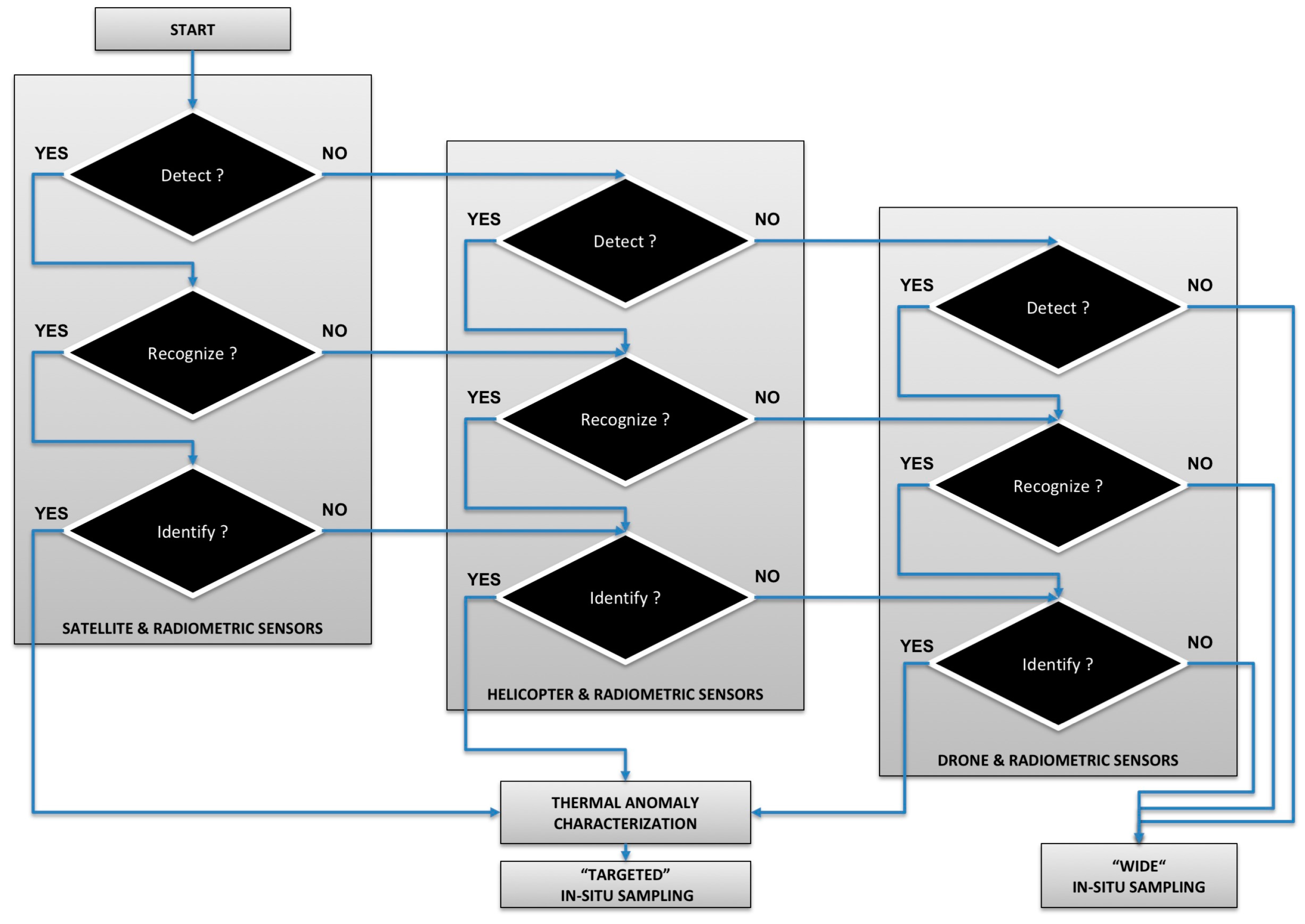
The hierarchical monitoring used temporally and spatially overlapping satellite, helicopter, and drone platforms (Figure 1) in order to simultaneously obtain thermal images of the targets (Figure 1). The selection of an imaging platform for water quality monitoring is based on the suitability of platform characteristics (Table 1) to detect, recognize, and identify criteria for characterizing the thermal anomalies of the plume (Figure 2). These criteria are specific to each sensor and target, and may involve: ratios of image spatial resolution or image swath size to the target size; matching of image spectral resolution to target thermal properties; and time to achieve target image relative to target time constraints. In cases where a thermal imaging platform is suitable, targeted, overlapping in situ monitoring may be deployed; otherwise un-targeted, wide in situ sampling might be used. The first step of the hierarchical monitoring was coordinating with flight dates for Landsat-8. After each flight, the Landsat imagery was retrieved and reviewed for evidence of discharging plumes, noted by different reflectance than the seawater, from the channels into the coastal zone. Evidence of discharging plumes was identified in the Landsat-8 images obtained on 18 June 2013, both in the natural look and TIRS band 10 thermal imagery. Given plume detection with Landsat-8, the second step in hierarchical monitoring was deployment of the helicopter, drone, and field boat, either immediately, or to coincide with the next Landsat-8 flight. In this project all monitoring was coordinated to temporally overlap with the Landsat-8 flight date of 27 June 2013. The helicopter was a rotorcraft AW139 (Augusta Westland, Rome, Italy), with a pilot and photographer, and acquired imagery at a flight acquisition of 300 m, with Star SAFIRE QWIP (FLIR, USA) + FLIR T620 camera (FLIR, USA), providing images with ~10 cm resolution. The unmanned drone was a StillFly 6–R Natural Drone (San Diego, CA, USA), and acquired imagery at a flight acquisition of 50 m with a FLIR T620, providing resolution with ~2 cm resolution [24,25]. The thermal cameras used by the helicopter and drone missions used a constant emissivity value of 0.986, and were set for ambient parameters in the thermal sensor control software, including atmospheric temperature, relative humidity, and distance, which was used by the T620 camera to compensate for the atmospheric interference and provide an accuracy of 2 mK in the measurements. Images were rejected if they had poor view angles (e.g., too oblique) and if they had extreme solar reflection off the water surface.
The in situ samples were coordinated to spatially and temporally overlap with the thermal imagery about the discharge plumes (Figure 3). A field boat was provided by the Regional Agency for the Environmental Protection and it carried an Ocean Seven 320 Plus multi-parameter Conductivity Temperature Depth (CTD) probe. The boat was used for in situ sampling to test the correlation with Trad, however, once this was performed subsequent monitoring would not require the costly concurrent collection of in situ samples. To coordinate the spatial congruence of the in situ sampling and proximal sensing, the operator of the field boat navigated to the coordinates of the areas of interest where thermal anomalies in the water were detected, with coordinates sent by radio between the helicopter and boat crews. The CTD in situ samples provided measurement of water kinetic temperature, Tkin, salinity, dissolved oxygen, chlorophyll-a, and turbidity. The CTD records were acquired at a frequency of 24 Hz, the highest allowed by the probes, taking the surficial measurements at 50 cm from the surface. During the CTD acquisitions the wind speeds measured 6 m/s at the weather station close to the sampling area, and this condition suggests the surface layer of the water was completely mixed with a homogeneous Tkin sampled at the 50 cm depth [26].
The third step of the monitoring program was to post-process the data and obtain the dataset of water quality and temperature. The thermographic imagery was post-processed to delineate the area of interest and obtain the average Trad value from that area, as well as other statistical data on the distribution of the Trad values. The in situ sampling provided one temperature parameter, Tkin, and the proximal sensing provided one temperature parameter, Trad, the combination of the two parameters allowed for a third parameter equal to the difference Tkin − Trad, and a fourth parameter of emissivity, ε, derived using the relationship between Tkin and Trad. An optional fourth step of the monitoring program was to post-process the imagery to define the edges of the areas of interest, where the plumes met with the coastal water. This involves extracting statistical information about the IR temperature spectra, defining standard thermal patterns related to the phenomenology of water pollution [27]. In this study, the consistent temperature difference along the perimeter suggested the edge of the channel plumes, which was confirmed with using Canny edge detection [28] (see image Figure 4 for the Volturno channel).
3. Results and Discussion
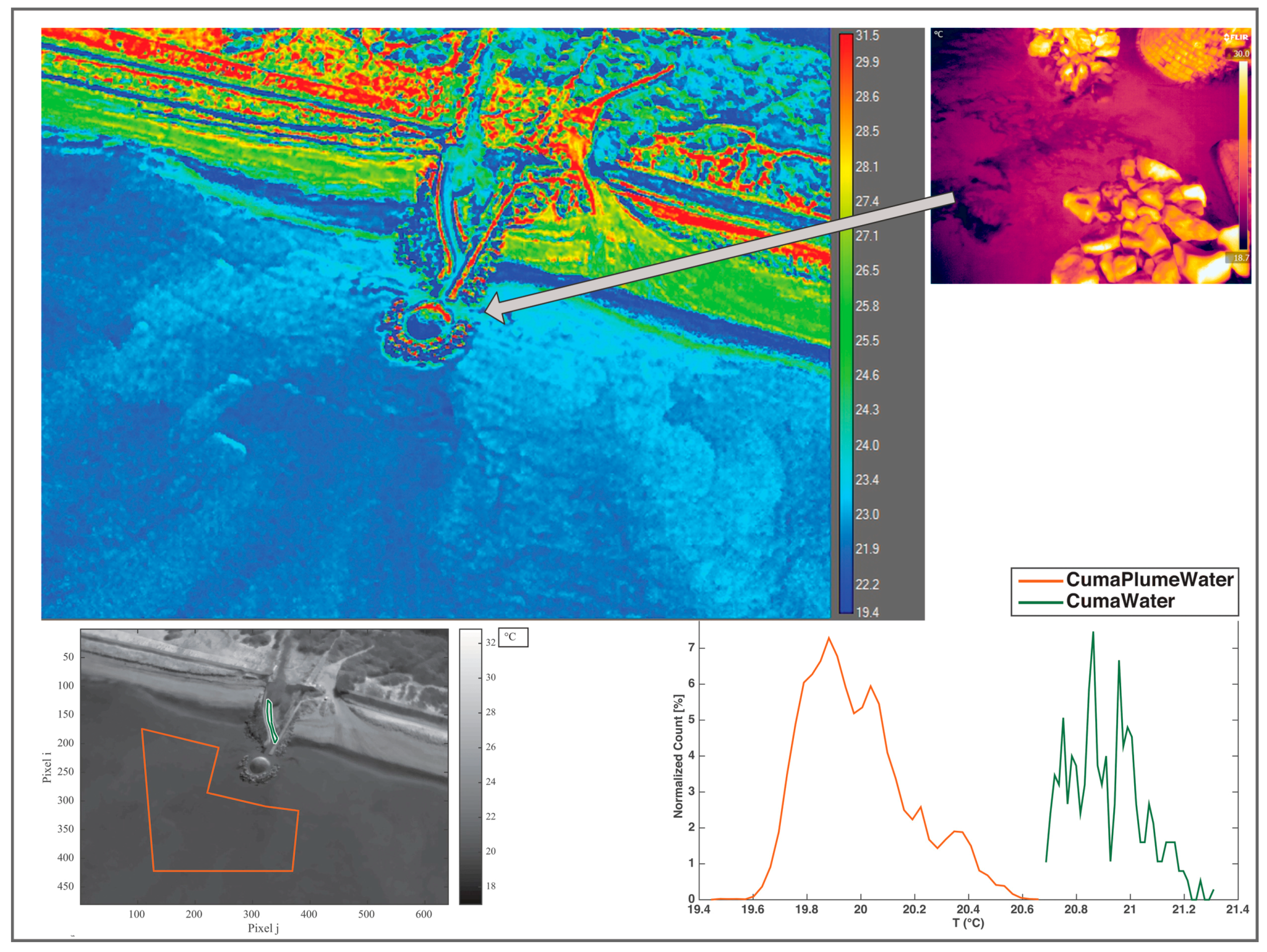
Plumes discharging from the four channels into the coastal waters were observed and captured with the helicopter thermographic camera. To capture the largest plume from the Volturno channel, with a channel width of ~300 m, the helicopter was used to take an oblique image (Figure 4), while less oblique images were used for the Agnena plume (Figure 5), Regi-Lagni plume (Figure 6), and the Cuma plume (Figure 7). The Cuma channel width was ~3 m, sufficient to allow for an area of interest to be delineated in the channel using the helicopter-acquired ~10 cm thermographic image. For more detailed analysis of the mixing zone between the Cuma channel discharge and coastal water, the drone-acquired ~2 cm thermographic image provides excellent detail (Figure 7). The Landsat-8 imagery performed its function as a first step of the hierarchical monitoring, and was sufficient to confirm that spectral differences existed along the coastal zone, and initiated the subsequent monitoring step 2, proximal image collection, and step 3, image post-processing, in the hierarchical program.
The in situ water quality measurements were obtained for one sample of coastal seawater beyond the plumes, one sample in the Volterno plume, one sample in the Agnena plume, two samples in the Regi Lagni plume, and two samples in the Cuma plume (Figure 3, Table 2). The salinity of the coastal seawater was 3.4% (i.e., 34 parts per thousand), while the salinity of plumes had a maximum of 3.7% and a minimum of 2.7%. The chlorophyll-a of the coastal seawater was 0.93 μg/L, while the chlorophyll-a of plumes had a maximum of 2.5 μg/L and a minimum of 0.97 μg/L. The dissolved oxygen of the coastal seawater was 87% of saturation, while the dissolved oxygen of plumes had a maximum of 107% and a minimum of 59.3%. The detection of dissolved oxygen above 100% saturation is relatively common in coastal sites due to the production of pure oxygen by photosynthetically-active organisms, as well as a momentary lack of equilibrium of dissolved oxygen between the water column and air column. The turbidity of the coastal seawater was 0.93 FTU (Formazin turbidity unit), while the turbidity of plumes had a maximum of 5.6 FTU and a minimum of 0.9 FTU. The kinetic temperature of the coastal seawater was 22.1 °C, while the kinetic temperature of plumes had a maximum of 23.7 °C and a minimum of 21.9 °C.
The kinetic temperature, Tkin, measured by the CTD in situ, and the radiometric temperature, Trad, measured from IR imagery, were used with Equation (4) to derive the emissivity, ε, for the areas of interest (Table 3). The derived ε values ranged from 0.93 to 0.97, with seawater at 0.97; this seawater ε value deviates from the standard of 0.98 and illustrates that ε can vary around a common value due to the variation in environmental and viewing conditions [29,30]. The Tkin, Trad, the difference Tkin − Trad, and the ε for each area of interest was correlated with the water quality parameters (Table 4). The correlations with in situ water quality data were consistently the best for the parameters of Tkin, Trad and ε, which were identical, or within 0.01 of each other, and worst for the parameter of Tkin. The absolute values of the Trad correlations were just 0.02 to 0.06 below the absolute values of the ε correlations, and 0.21 to 0.36 higher than the absolute values of the Tkin correlations. Given that parameterizing ε and Tkin requires in situ measurement, the Trad correlations were of particular interest because Trad can be collected remotely and expedite monitoring. For in situ salinity Trad had a correlation of 0.81, for chlorophyll-a Trad had a correlation of 0.74, for dissolved oxygen Trad had a correlation of 0.98, and for turbidity Trad had a correlation of −0.61.
In the Regi Lagni channel there was no detected difference between the channel continental water and the seawater mixing zone water, attributed to a more complete mixing along this section of the coast. All channels had a relatively low discharge during the warm season, with water temperatures warmer than the seawater for all channels, but the larger Volturno, which drains a larger river basin with high-altitude tributaries that may feed cooler water. The smallest channel, the ~3 m wide Cuma, had the highest levels of chlorophyll-a, while the medium sized channel, the ~100 m wide Regi Lagni, had the next highest levels of chlorophyll-a, suggesting they may be the most polluted channels. The reported values of oxygen under saturation suggest the presence of a high level of photosynthesis, and the Cuma channel had the highest chlorophyll-a and second highest dissolved oxygen values. The high turbidity values from all channels, above the 0.93 FTU of the seawater, suggest the channels are carrying a high concentration of particulate matter, which may carry additional contamination.
The two temperature variables that correlated best with water quality parameters, the difference Tkin and Trad and ε, which is from a ratio of Tkin and Trad, are based on using both kinetic and radiometric temperatures. However, in typical applications of this monitoring program the Tkin and ε will not be available. Only with in situ measurements will Tkin be available, and only with Tkin can ε be derived, As intended in this study, Trad is the most available temperature parameter from this monitoring program, and in this application it had a much stronger correlation with the water quality parameters than the Tkin. The Trad correlations were, on average, 71% better than the Tkin correlations, and ranged from 144% better for turbidity to 27% better for oxygen. The Trad correlations were all above 0.6, and three were above 0.74, while three of the Tkin correlations were below 0.51.
The study demonstrates how thermographic data can support a coastal monitoring program that targets the water quality impact of channel plumes discharge along the coast. This study addressed the research question by establishing a strong correlation between Trad and four common water quality parameters. In a subsequent application of this hierarchical monitoring program, the second step would not require a concurrent field boat with in situ sampling and, instead, would just collect Trad for areas of interest within the thermographic imagery acquired by the helicopter and/or drone. If the plumes and seawater areas had different values of Trad for any one channel, then in situ samples could subsequently be obtained to characterize the water quality. The limitations of the monitoring program include the inability to estimate the water quality parameter concentration using the Trad, and predictive equations are difficult to establish given the sensitivity of Trad to variation in ambient air temperature, water temperature, and emissivity of the pollutant. At sites where thermographic data alone are insufficient for the monitoring program, other approaches have been used. The fusion of optical data and synthetic aperture radar have been used for feature-based detection of environmental hazards [31,32], and ratios of multi-spectral bands have been used to detect surface contamination of soil and water [33,34]. Monitoring programs can also use remote sensing-based detection cyanobacteria together with knowledge of flow paths to make inferences of the impact and source of water pollution [35].
Without the hierarchical monitoring via helicopter, prior coastal monitoring for this region limited its focus to pollution from the largest channels, including the Volturno, and another large channel further north, called the Garigliano [36,37,38,39]. Due to the larger discharge plumes from these rivers, they have been considered to be the principal cause of water quality impairment. This research revealed that the smallest channel, the Cuma, and the medium-sized channel, the Regi Lagni, had the highest concentrations of chlorophyll-a, which can lead to significant local degradation of coastal water quality. Indeed, the contaminant concentrations from the small channels originate with wastewater treatment and agricultural runoff, and can be higher than those of the larger rivers. The lower flow rates from these small channels do not generate significant plume dispersion, and constrain the dilution and degradation of the pollutant during transport. During the warm season the coastal currents are mostly onshore, due to local land-sea breezes, and the river discharge and pollutants are retained in the littoral area.
In summary, the hierarchical sampling protocol might search for thermal anomalies first using satellite data, if the channel width is large enough, and then proceed to helicopter or drone data depending on channel size and distance between channels. Collaboration between teams with environmental expertise and teams with access to helicopters and drones may be critical to combine resources and complete the monitoring program. The collaboration with governmental authorities for access to helicopters can satisfy their needs for pollution monitoring, and ideally fit within their operational requirements in terms of both flight regulations and the mission goals, while satisfying the scientific aims and requirements to analyze the data. The application of this methodology produces multi-resolution data that can be processed to highlight thermal anomalies, and the inferences with respect to water quality are enhanced using local knowledge of pollutant sources. Indeed, with a proper knowledge of the environmental dynamics, such as the interaction of the channels and coastal currents, this application can link thermal anomalies and environmental criticalities.
4. Conclusions
This research demonstrated that a hierarchical use of remotely-sensed imagery from satellites, then helicopter, and then proximal sensed imagery from drones, provides a range of spatial and temporal coverage to support water quality monitoring of complex pollution scenarios. The research established that the thermal infrared cameras can be used in the monitoring of water quality anomalies, with the radiometric temperature, Trad, strongly correlating with water quality parameters of salinity, chlorophyll-a, dissolved oxygen, and turbidity. The Landsat-8 remotely-sensed imagery was used as a first step to identify that plumes were discharging into the coastal water. The helicopter was used as a second step to obtain proximal imagery with a spatial resolution of ~10 cm, able to sample the plumes discharging from ~300 to ~3 m channels. The area of interest in the proximal thermal imagery captured Trad values that had a correlation of 0.81 with salinity, of 0.74 with chlorophyll-a, 0.98 with dissolved oxygen, and −0.61 with turbidity. This study demonstrates the utility of using thermal imagery in cases where more advanced monitoring is unable due to spatial, temporal, and financial constraints.
Acknowledgments
We acknowledge the Italian Governmental Authorities, and the ARPA Campania and the director of the Marine Protection and Oceanography division, Lucio De Maio, for providing their instrumentation for in situ measurements. We recognize the support of CINFAI and RITMARE Project, funded by the Italian Ministry of University and Research. The last two authors are grateful to the US and Italian Fulbright Commission and Parthenope University of Naples for sponsoring their collaboration with the Italian research partners. Massimiliano Lega and Giannetta Fusco acknowledge the financial support received by Università degli Studi di Napoli ‘Parthenope’ under “Bando di sostegno alla ricerca individuale per il triennio 2015–2017”.
Author Contributions
M.L. and P.B. conceived and designed the experiments; G.F. coordinated the in situ sampling; M.L. coordinated the proximal sensing; C.F. and T.E. post-processed and analyzed the data; and C.F., M.L., and T.E. wrote the paper.
Conflicts of Interest
The authors declare no conflict of interest. The founding sponsors had no role in the design of the study; in the collection, analyses, or interpretation of data; in the writing of the manuscript, and in the decision to publish the results.
References
- Ahn, Y.H.; Shanmugam, P.; Lee, J.H.; Kang, Y.Q. Application of satellite infrared data for mapping of thermal plume contamination in coastal ecosystem of Korea. Mar. Environ. Res. 2006, 61, 186–201. [Google Scholar] [CrossRef] [PubMed]
- Hook, S.J.; Chander, G.; Barsi, J.A.; Alley, R.E.; Abtahi, A.; Palluconi, F.D.; Markham, B.L.; Richards, R.C.; Schladow, S.G.; Helder, D.L. In-flight validation and recovery of water surface temperature with Landsat-5 thermal infrared data using an automated high-altitude lake validation site at Lake Tahoe. IEEE Trans. Geosci. Remote Sens. 2004, 42, 2767–2776. [Google Scholar] [CrossRef]
- Hedger, R.D.; Malthus, T.J.; Folkard, A.M. Estimation of velocity fields at the estuary-coastal interface through statistical analysis of successive airborne remotely sensed images. Int. J. Remote Sens. 2001, 22, 3901–3906. [Google Scholar] [CrossRef]
- El Din, E.S.; Zhang, Y.; Suliman, A. Mapping concentrations of surface water quality parameters using a novel remote sensing and artificial intelligence framework. Int. J. Remote Sens. 2017, 38, 1023–1042. [Google Scholar] [CrossRef]
- Jansen, J.R. Remote Sensing of the Environment: An Earth Resource Perspective, 2nd ed.; Pearson: New York, NY, USA, 2006; p. 608. [Google Scholar]
- Gholizadeh, M.H.; Melesse, A.M.; Reddi, L. Spaceborne and airborne sensors in water quality assessment. Int. J. Remote Sens. 2016, 37, 3143–3180. [Google Scholar] [CrossRef]
- Brando, V.E.; Dekker, A.G. Satellite hyperspectral remote sensing for estimating estuarine and coastal water quality. IEEE Trans. Geosci. Remote Sens. 2003, 41, 1378–1387. [Google Scholar] [CrossRef]
- Keith, D.J.; Schaeffer, B.A.; Lunetta, R.S.; Rocha, K.; Cobb, D.J.; Gould, R.W., Jr. Remote sensing of selected water-quality indicators with the hyperspectral imager for the coastal ocean (HICO) sensor. Int. J. Remote Sens. 2014, 35, 2927–2962. [Google Scholar] [CrossRef]
- Chung, W.Y.; Yoo, J.H. Remote water quality monitoring in wide area. Sens. Actuators B Chem. 2015, 217, 51–57. [Google Scholar] [CrossRef]
- Czajkowski, K.P.; Goward, S.N.; Stadler, S.J.; Walz, A. Thermal remote sensing of near surface environmental variables: Application over the Oklahoma Mesonet. Prof. Geogr. 2000, 52, 345–357. [Google Scholar] [CrossRef]
- Wooster, M.J.; Roberts, G.; Smith, A.; Johnston, J.; Freeborn, P.; Amici, S.; Hudak, A. Thermal remote sensing of active vegetation fires and biomass burning events. In Thermal Infrared Remote Sensing: Sensors, Methods, Applications; Kuenzer, C., Dech, S., Eds.; Springer: Dordrecht, The Netherlands; Heidelberg, Germany; New York, NY, USA, 2013; pp. 347–390. [Google Scholar]
- Kuenzer, C.; Dech, S. Theoretical background of thermal infrared remote sensing. In Thermal Infrared Remote Sensing: Sensors, Methods, Applications; Kuenzer, C., Dech, S., Eds.; Springer: Dordrecht, The Netherlands; Heidelberg, Germany; New York, NY, USA, 2013; pp. 1–26. [Google Scholar]
- Branch, R.; Chickadel, C.C.; Jessup, A.T. Infrared emissivity of seawater and foam at large incidence angles in the 3–14 mu m wavelength range. Remote Sens. Environ. 2016, 184, 15–24. [Google Scholar] [CrossRef]
- Niclos, R.; Caselles, V.; Coll, C.; Valor, E.; Rubio, E. Autonomous measurements of sea surface temperature using in situ thermal infrared data. J. Atmos. Ocean. Technol. 2004, 21, 683–692. [Google Scholar] [CrossRef]
- Cotroneo, Y.; Aulicino, G.; Ruiz, S.; Pascual, A.; Budillon, G.; Fusco, G.; Tintoré, J. Glider and satellite high resolution monitoring of a mesoscale eddy in the algerian basin: Effects on the mixed layer depth and biochemistry. J. Mar. Syst. 2016, 162, 73–88. [Google Scholar] [CrossRef]
- Aulicino, G.; Cotroneo, Y.; Lacava, T.; Sileo, G.; Fusco, G.; Carlon, R.; Budillon, G. Results of the first Wave Glider experiment in the southern Tyrrhenian Sea. Adv. Oceanogr. Limnol. 2016, 7. [Google Scholar] [CrossRef]
- Norman, J.M.; Becker, F. Terminology in Thermal Infrared Remote-sensing of Natural Surfaces. Agric. For. Meteorol. 1995, 77, 153–166. [Google Scholar] [CrossRef]
- Li, Z.L.; Wu, H.; Wang, N.; Qiu, S.; Sobrino, J.A.; Wan, Z.; Tang, B.H.; Yan, G. Land surface emissivity retrieval from satellite data. Int. J. Remote Sens. 2013, 34, 3084–3127. [Google Scholar] [CrossRef]
- Lega, M.; Kosmatka, J.; Ferrara, C.; Russo, F.; Napoli, R.M.A.; Persechino, G. Using Advanced Aerial Platforms and Infrared Thermography to Track Environmental Contamination. Environ. Forensics 2012, 13, 332–338. [Google Scholar] [CrossRef]
- Lindenmayer, D.B.; Likens, G.E. The science and application of ecological monitoring. Biol. Conserv. 2010, 143, 1317–1328. [Google Scholar] [CrossRef]
- Wikle, C.K. Hierarchical models in environmental science. Int. Stat. Rev. 2003, 71, 181–199. [Google Scholar] [CrossRef]
- De Maio, A.; Moretti, M.; Sansone, E.; Spezie, G.; Vultaggio, M. Outline of Marine Currents in the Bay of Naples and Some Considerations on Pollutant Transport. Nuovo Cimento Della Societa Ital. Di Fisica C-Geophys. Space Phys. 1985, 8, 955–969. [Google Scholar] [CrossRef]
- Carrada, G.C.; Hopkins, T.S.; Bonaduce, G.; Ianora, A.; Marino, D.; Modigh, M.; Ribera, D.A.M.; Scotto, C.B. Variability in the Hydrographic and Biological Features of the Gulf of Naples. Mar. Ecol. 1980, 1, 105–120. [Google Scholar] [CrossRef]
- Lega, M.; Napoli, R.M.A. Aerial infrared thermography in the surface waters contamination monitoring. Desalination Water Treat. 2010, 23, 141–151. [Google Scholar] [CrossRef]
- Lega, M.; Ferrara, C.; Persechino, G.; Bishop, P. Remote sensing in environmental police investigations: Aerial platforms and an innovative application of thermography to detect several illegal activities. Environ. Monit. Assess. 2014, 186, 8291–8301. [Google Scholar] [CrossRef] [PubMed]
- Brainerd, K.E.; Gregg, M.C. Surface Mixed and Mixing Layer Depths. Deep-Sea Res. Part I-Oceanogr. Res. Pap. 1995, 42, 1521–1543. [Google Scholar] [CrossRef]
- Lega, M.; Persechino, G. GIS and Infrared Aerial View: Advanced Tools for the Early Detection of Environmental Violations. WIT Trans. Ecol. Environ. 2014, 180, 225–235. [Google Scholar]
- Canny, J. A Computational Approach to Edge-detection. IEEE Trans. Pattern Anal. Mach. Intell. 1986, 8, 679–698. [Google Scholar] [CrossRef] [PubMed]
- Sidran, M. Broadband reflectance and emissivity of specular and rough water surfaces. Appl. Opt. 1981, 20, 3176–3183. [Google Scholar] [CrossRef] [PubMed]
- Smith, W.L.; Knuteson, R.O.; Revercomb, H.E.; Feltz, W.; Nalli, N.R.; Howell, H.B.; Menzel, W.P.; Brown, O.; Brown, J.; Minnett, P.; et al. Observations of the Infrared Radiative Properties of the Ocean—Implications for the Measurement of Sea Surface Temperature via Satellite Remote Sensing. Bull. Am. Meteorol. Soc. 1996, 77, 41–51. [Google Scholar] [CrossRef]
- Errico, A.; Angelino, C.V.; Cicala, L.; Podobinski, D.P.; Persechino, G.; Ferrara, C.; Lega, M.; Vallario, A.; Parente, C.; Masi, G.; et al. SAR/multispectral image fusion for the detection of environmental hazards with a GIS. In Proceedings of the SPIE Remote Sensing, Amsterdam, The Netherlands, 23–25 September 2014; International Society for Optics and Photonics: Bellingham, WA, USA; p. 924503. [Google Scholar] [CrossRef]
- Errico, A.; Angelino, C.V.; Cicala, L.; Persechino, G.; Ferrara, C.; Lega, M.; Vallario, A.; Parente, C.; Masi, G.; Gaetano, R.; et al. Detection of environmental hazards through the feature-based fusion of optical and SAR data: A case study in southern Italy. Int. J. Remote Sens. 2015, 36, 3345–3367. [Google Scholar] [CrossRef]
- Lega, M.; D’antonio, L.; Napoli, R.M. Cultural Heritage and Waste Heritage: Advanced techniques to preserve cultural heritage, exploring just in time the ruins produced by disasters and natural calamities. In Waste Management and the Environment V; Popov, V., Itoh, H., Mander, U., Brebbia, C.A., Eds.; WIT Press: Southampton, UK; Billerica, MA, USA, 2010; pp. 123–134. [Google Scholar]
- Lega, M.; Endreny, T. Quantifying the environmental impact of pollutant plumes from coastal rivers with remote sensing and river basin modelling. Int. J. Sustain. Dev. Plan. 2016, 11, 651–662. [Google Scholar] [CrossRef]
- Teta, R.; Romano, V.; Della Sala, G.; Picchio, S.; De Sterlich, C.; Mangoni, A.; Di Tullio, G.; Costantino, V.; Lega, M. Cyanobacteria as indicators of water quality in Campania coasts, Italy: A monitoring strategy combining remote/proximal sensing and in situ data. Environ. Res. Lett. 2017, 12, 024001. [Google Scholar] [CrossRef]
- Isidori, M.; Lavorgna, M.; Nardelli, A.; Parrella, A. Integrated environmental assessment of Volturno River in South Italy. Sci. Total Environ. 2004, 327, 123–134. [Google Scholar] [CrossRef] [PubMed]
- De Pippo, T.; Donadio, C.; Pennetta, M.; Petrosino, C.; Terlizzi, F.; Valente, A. Coastal hazard assessment and mapping in Northern Campania. Italy Geomorphol 2008, 97, 451–466. [Google Scholar] [CrossRef]
- Infascelli, R.; Pelorosso, R.; Boccia, L. Spatial assessment of animal manure spreading and groundwater nitrate pollution. Geospat. Health 2009, 4, 27–38. [Google Scholar] [CrossRef] [PubMed]
- Amodiococchieri, R.; Arnese, A. Organochlorine Pesticide-residues in Fish from Southern Italian Rivers. Bull. Environ. Contam. Toxicol. 1988, 40, 233–239. [Google Scholar] [CrossRef]
Figure 1.
Illustration of the hierarchical monitoring program using (A) satellite, (B) helicopter, (C) drone and (D) field boat to study the mixing of channel plumes in the coastal zone.
Figure 1.
Illustration of the hierarchical monitoring program using (A) satellite, (B) helicopter, (C) drone and (D) field boat to study the mixing of channel plumes in the coastal zone.

Figure 2.
Flowchart illustrating the choice of platform in hierarchical monitoring, related to target detect, recognize, and identify criteria. All three platforms may be needed for a set of distinct targets.
Figure 2.
Flowchart illustrating the choice of platform in hierarchical monitoring, related to target detect, recognize, and identify criteria. All three platforms may be needed for a set of distinct targets.

Figure 3.
Landsat-8 image of the study area with dots indicating the location of the field boat sampling sites, within the channel discharge areas of interest.
Figure 3.
Landsat-8 image of the study area with dots indicating the location of the field boat sampling sites, within the channel discharge areas of interest.
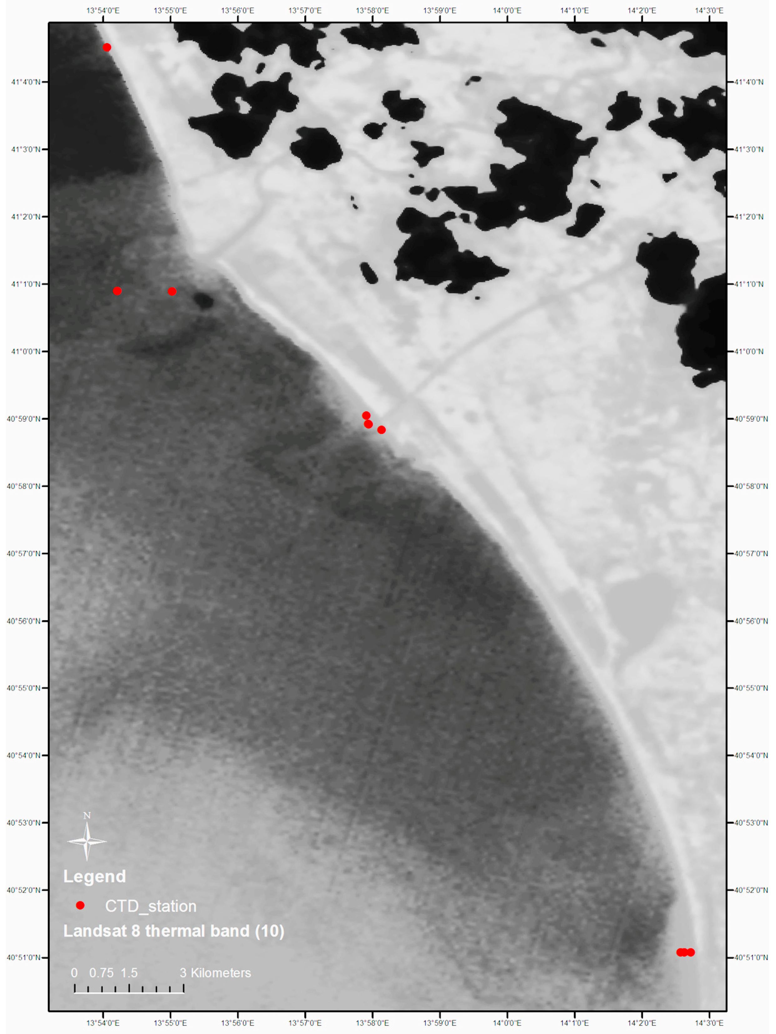
Figure 4.
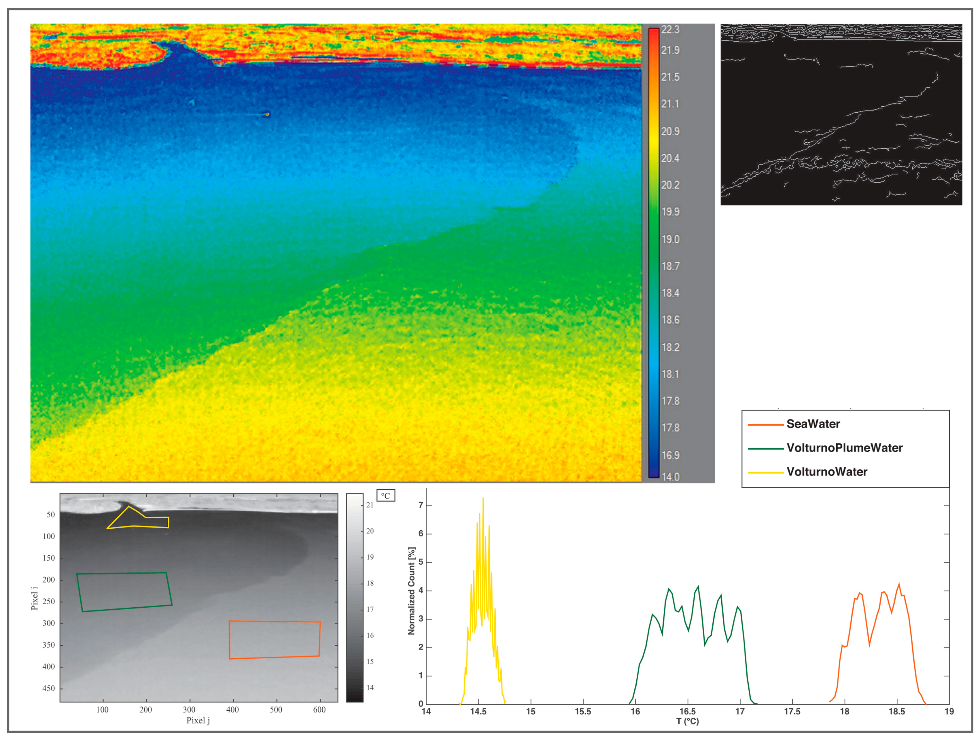
Thermal image of the Volturno plume with polygons over the channel, seawater, and plume areas of interest, which correspond to histograms of radiometric temperature; and (upper right side) edges of the Volturno channel plume as white lines to the right of the image.
Figure 4.
Thermal image of the Volturno plume with polygons over the channel, seawater, and plume areas of interest, which correspond to histograms of radiometric temperature; and (upper right side) edges of the Volturno channel plume as white lines to the right of the image.

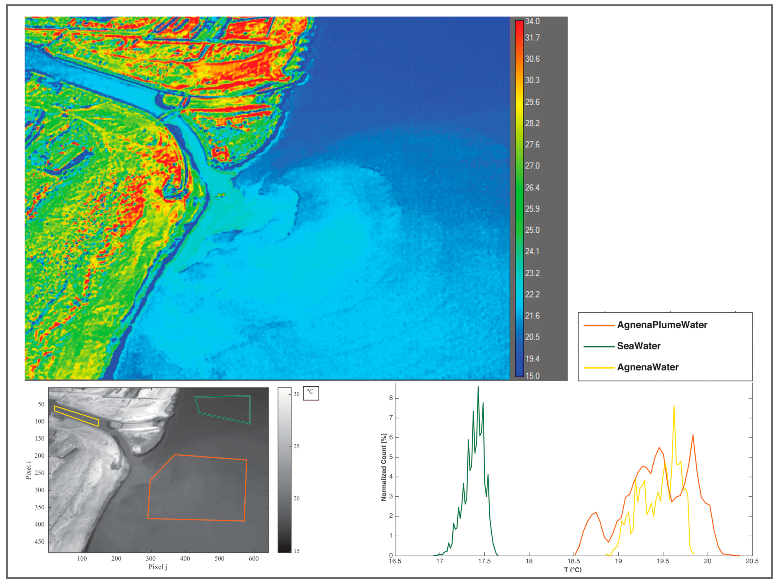
Figure 5.
Thermal image of Agnena plume with histogram of radiometric temperature for areas of the channel, seawater and area of the plume.
Figure 5.
Thermal image of Agnena plume with histogram of radiometric temperature for areas of the channel, seawater and area of the plume.

Figure 6.
Thermal image of Regi Lagni plume with histogram of radiometric temperature for areas of the channel, seawater, and area of the plume.
Figure 6.
Thermal image of Regi Lagni plume with histogram of radiometric temperature for areas of the channel, seawater, and area of the plume.
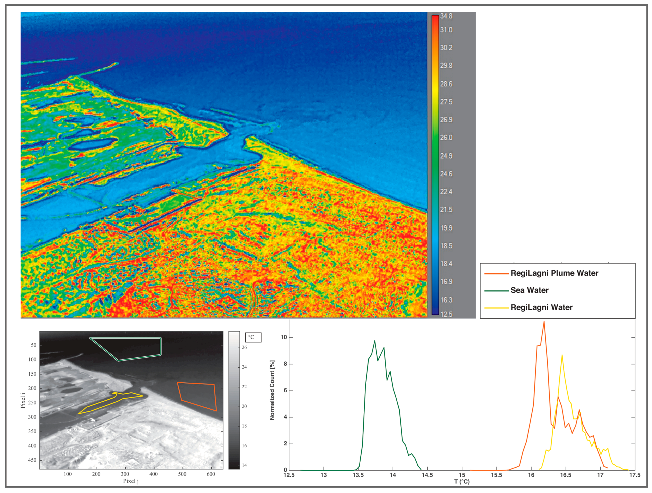
Figure 7.
Thermal image of Cuma plume with histogram of radiometric temperature for areas of the channel, seawater, and area of the plume; and (in upper right side) drone-acquired thermal image of the mixing zone in the Cuma channel outlet.
Figure 7.
Thermal image of Cuma plume with histogram of radiometric temperature for areas of the channel, seawater, and area of the plume; and (in upper right side) drone-acquired thermal image of the mixing zone in the Cuma channel outlet.

Table 1.
Hierarchical monitoring platforms of satellite, helicopter, and drone, with the associated thermal image sensor, target distance, swath size, spatial resolution, and spectral resolution.
Table 1.
Hierarchical monitoring platforms of satellite, helicopter, and drone, with the associated thermal image sensor, target distance, swath size, spatial resolution, and spectral resolution.
| Hierarchical Monitoring Platform | Thermal Image Sensor | Target Distance (km) | Image Swath Size (km) | Image Spatial Resolution (m) | Image Spectral Resolution (μm) |
|---|---|---|---|---|---|
| Satellite | Landsat 8 TIRS | 705 | 190 | 100 | Band 10: 10.60–11.19 |
| Helicopter | FLIR T620 | 0.3 | ~4.7 | 0.12 | 7–14 |
| Drone | FLIR T620 | 0.05 | ~0.13 | 0.02 | 7–14 |
Table 2.
Water quality parameters measured during the in situ field campaign, with salinity in %, chlorophyll-a in μg/L, dissolved oxygen (DO) in % saturation, turbidity in Formazin turbidity units (FTU), and kinetic temperature in °C.
Table 2.
Water quality parameters measured during the in situ field campaign, with salinity in %, chlorophyll-a in μg/L, dissolved oxygen (DO) in % saturation, turbidity in Formazin turbidity units (FTU), and kinetic temperature in °C.
| Locations | Salinity % | Chl-a μg/L | DO% Sat | Turbidity FTU | Tkin °C |
|---|---|---|---|---|---|
| Volturno Plume | 3.4 | 0.97 | 107 | 1.70 | 21.90 |
| Agnena Plume | 3.7 | 0.55 | 87 | 2.05 | 22.10 |
| Regi Lagni Plume 1 | 3.3 | 2.20 | 65 | 2.29 | 22.48 |
| Regi Lagni Plume 2 | 2.7 | 1.66 | 59 | 5.65 | 22.90 |
| Cuma Plume 1 | 3.7 | 2.25 | 100 | 1.94 | 23.06 |
| Cuma Plume 2 | 3.7 | 2.51 | 102 | 1.94 | 23.65 |
| Coastal Seawater | 3.4 | 0.93 | 87 | 0.93 | 22.10 |
Table 3.
Water in situ kinetic temperature, Tkin (°C), IR thermographic radiometric temperature, Trad (°C), the difference of Tkin and Trad, and the derived emissivity, ε, for the areas of interest.
Table 3.
Water in situ kinetic temperature, Tkin (°C), IR thermographic radiometric temperature, Trad (°C), the difference of Tkin and Trad, and the derived emissivity, ε, for the areas of interest.
| Locations | Tkin °C | Trad °C | Tkin − Trad °C | ε |
|---|---|---|---|---|
| Volturno Plume | 21.90 | 17.50 | 4.40 | 0.942 |
| Agnena Plume | 22.10 | 19.90 | 2.20 | 0.971 |
| Regi Lagni Plume 1 | 22.48 | 17.10 | 5.38 | 0.929 |
| Regi Lagni Plume 2 | 22.90 | 17.30 | 5.60 | 0.926 |
| Cuma Plume 1 | 23.06 | 20.08 | 2.98 | 0.960 |
| Cuma Plume 2 | 23.65 | 20.90 | 2.75 | 0.963 |
| Coastal Seawater | 22.10 | 19.90 | 2.20 | 0.971 |
Table 4.
Correlation coefficients between water quality parameters salinity (%), chlorophyll-a (μg/L), dissolved oxygen (DO, % saturation), turbidity (Formazin turbidity units, FTU), and in situ kinetic temperature, Tkin (°C), IR thermographic radiometric temperature, Trad (°C), the difference of Tkin and Trad, and the derived emissivity, ε, for the areas of interest.
| Variables | Salinity % | Chl-a μg/L | DO %Sat | Turbidity FTU |
|---|---|---|---|---|
| Tkin | 0.48 | 0.51 | 0.77 | −0.25 |
| Trad | 0.81 | 0.74 | 0.98 | −0.61 |
| Tkin − Trad | −0.87 | −0.78 | −1.00 | 0.69 |
| ε | 0.86 | 0.77 | 1.00 | −0.67 |
© 2017 by the authors. Licensee MDPI, Basel, Switzerland. This article is an open access article distributed under the terms and conditions of the Creative Commons Attribution (CC BY) license (http://creativecommons.org/licenses/by/4.0/).
Share and Cite
MDPI and ACS Style
Ferrara, C.; Lega, M.; Fusco, G.; Bishop, P.; Endreny, T. Characterization of Terrestrial Discharges into Coastal Waters with Thermal Imagery from a Hierarchical Monitoring Program. Water 2017, 9, 500. https://doi.org/10.3390/w9070500
AMA Style
Ferrara C, Lega M, Fusco G, Bishop P, Endreny T. Characterization of Terrestrial Discharges into Coastal Waters with Thermal Imagery from a Hierarchical Monitoring Program. Water. 2017; 9(7):500. https://doi.org/10.3390/w9070500
Chicago/Turabian StyleFerrara, Claudia, Massimiliano Lega, Giannetta Fusco, Paul Bishop, and Theodore Endreny. 2017. "Characterization of Terrestrial Discharges into Coastal Waters with Thermal Imagery from a Hierarchical Monitoring Program" Water 9, no. 7: 500. https://doi.org/10.3390/w9070500
Note that from the first issue of 2016, this journal uses article numbers instead of page numbers. See further details here.