Article

Characterisation of Hydrological Response to Rainfall at Multi Spatio-Temporal Scales in Savannas of Semi-Arid Australia

1
Sustainability Research Centre, University of the Sunshine Coast, Sunshine Coast, Queensland 4556, Australia
2
CSIRO Land and Water, Brisbane, Queensland 4102, Australia
3
CSIRO Land and Water, Canberra 2601, Australia
*
Author to whom correspondence should be addressed.
Water 2017, 9(7), 540; https://doi.org/10.3390/w9070540
Submission received: 30 March 2017 / Revised: 13 July 2017 / Accepted: 14 July 2017 / Published: 19 July 2017

Abstract

:
Rainfall is the main driver of hydrological processes in dryland environments and characterising the rainfall variability and processes of runoff generation are critical for understanding ecosystem function of catchments. Using remote sensing and in situ data sets, we assess the spatial and temporal variability of the rainfall, rainfall–runoff response, and effects on runoff coefficients of antecedent soil moisture and ground cover at different spatial scales. This analysis was undertaken in the Upper Burdekin catchment, northeast Australia, which is a major contributor of sediment and nutrients to the Great Barrier Reef. The high temporal and spatial variability of rainfall are found to exert significant controls on runoff generation processes. Rainfall amount and intensity are the primary runoff controls, and runoff coefficients for wet antecedent conditions were higher than for dry conditions. The majority of runoff occurred via surface runoff generation mechanisms, with subsurface runoff likely contributing little runoff due to the intense nature of rainfall events. MODIS monthly ground cover data showed better results in distinguishing effects of ground cover on runoff that Landsat-derived seasonal ground cover data. We conclude that in the range of moderate to large catchments (193–36,260 km2) runoff generation processes are sensitive to both antecedent soil moisture and ground cover. A higher runoff–ground cover correlation in drier months with sparse ground cover highlighted the critical role of cover at the onset of the wet season (driest period) and how runoff generation is more sensitive to cover in drier months than in wetter months. The monthly water balance analysis indicates that runoff generation in wetter months (January and February) is partially influenced by saturation overland flow, most likely confined to saturated soils in riparian corridors, swales, and areas of shallow soil. By March and continuing through October, the soil “bucket” progressively empties by evapotranspiration, and Hortonian overland flow becomes the dominant, if not exclusive, flow generation process. The results of this study can be used to better understand the rainfall–runoff relationships in dryland environments and subsequent exposure of coral reef ecosystems in Australia and elsewhere to terrestrial runoff.

1. Introduction

The world’s coral reefs have undoubtedly been subjected to natural and anthropogenic disturbances and are being degraded [1,2,3,4,5,6]. It is now well established that the ecological health of the coral reefs is under stress from threats associated with climate change and terrestrial runoff [2,3,4,5,7,8,9]. Runoff and the sediment and nutrients it carries are considered to be major factors causing deterioration in the health of the Great Barrier Reef (GBR) [1,3,10] and other coral reefs worldwide [2,4,5,11]. The GBR, a UNESCO world heritage site in northeastern Australia, is estimated to be worth ~$5.1 billion annually to the Australian economy, exceeding that of agricultural industries adjacent to the GBR [12]. A study of coral reefs between 2007 and 2013 concluded that live coral cover declined by 50% following several weeks of exposure to turbid water from major sediment plumes [13]. Terrestrial runoff, fluvial sediment and nutrient discharges are estimated to contribute the majority of the pollutants to the GBR lagoon in Australia and worldwide [2,11,14,15,16]. Therefore, in-depth investigations of the hydrological processes within these catchments are essential to understand the relationship among rainfall, land management and terrestrial runoff, and the subsequent impacts on pollutant generation and the ecological health of the coral reefs.
There have been a number of studies investigating different aspects of terrestrial runoff to the GBR. At smaller scales (i.e., plot), studies have established that annual runoff varies considerably with the spatial distribution of ground cover [17]; however, cover may have little effect on overland flow during very large rainfall events (>100 mm with intensities between 45 and 60 mm/h) when the landscape is inundated with surface runoff due to Hortonian overland flow processes [18,19,20]. Roth [21] showed that high ground cover values (>75%) can promote infiltration during high intensity events. Even with high cover, localised infiltration varied widely, mainly as a function of macroscopically visible bioturbation by soil macrofauna, such as ants, termites and earthworms. Ground cover is also very “patchy” in these savanna landscapes [22], which results in variable runoff coefficients even for hillslopes with the same overall cover conditions [17]. Livestock grazing is the dominant land use (~80%) in the catchments draining to the GBR. Therefore, understanding the effect of ground cover changes on runoff generation process is critical in those catchments.
At the larger (>100 km2) catchment scale, Post [23] regionalised rainfall–runoff (RR) model parameters to predict daily streamflow in ungauged catchments in the Burdekin River basin. A daily lumped parameter RR model (IHACRES) used regionalised model parameters based on catchment physiographic attributes for three portions of the basin: Upper Burdekin, Bowen, and Suttor/lower Burdekin [23]. Although average wet season and daily rainfall data over 24 catchments (68–130, 146 km2) were used, no spatial distribution of rainfall or ground cover was considered. Lough [24] used luminescent lines in corals to reconstruct the history (1685–1981) of major freshwater flows reaching the GBR from the Burdekin River. This study noted that the variability of rainfall and runoff increased during the 20th century, with more very wet and very dry extremes than previous periods [24]. Interestingly, trend analysis of stream flow records in northern Australia (Upper Burdekin catchment and Comet catchment) revealed only small impacts of woodland clearing (pre-clearing (1920–1953) compared to post-clearing (1979–2007)) on both mean and inter-annual streamflow. In the Upper Burdekin some of this increased variability may be the result of baseflow dynamics following tree clearing and increased storm flow during large events [25]. In particular, a series of La Nina events led to an unusual increase in runoff coefficients after clearing. In addition, during drought years (2002–2003) with no runoff, annual rainfall in Australian savannas is matched by annual evapotranspiration and trees extract water from deeper in the soil to maintain transpiration that exceeds rainfall [26]. The influence of ground cover on runoff and soil movement in small plots highlights the relationship between sparse (<40%) ground cover and runoff generation [19]. However, for very large events with high rainfall intensities (>100 mm/h), cover had little influence on runoff [18,19]. In all these aforementioned studies, only temporal variability of rainfall was considered, not spatial variability throughout the catchment. In our study, we assess both temporal and spatial patterns of rainfall to identify potential erosion hot spots. This will assist government departments in targeting critical parts of the catchment for remedial land management and erosion control practices.
Several studies in the GBR have shown that converting forest to pasture can increase runoff by ~80% at sub-catchment scales [27] and ~40% for river basin scales [28]. Importantly, all of these studies assessed only tree cover, and did not evaluate ground cover (pasture) amount and condition. Few studies assessed the link between pasture cover and runoff at property or sub-catchment scales because monitoring land management changes over long time scales (>10 years) is laborious and expensive; however, such long-term measurements are necessary to assess the large natural climate variability in semi-arid rangeland systems [29]. There is also a need to distinguish between the impacts of human activities and climate variability on runoff and sediment generation. As evidence of anthropogenic impacts on runoff, trends in ground cover changes were compared with trends in rainfall–runoff records.
Hydrological processes in the dry tropics differ from other regions as these ecosystems have greater energy inputs and faster rates of change [30]. Because precipitation is the dominant meteorological driver of runoff generation and soil erosion (including channel and gully erosion processes), analysis of rainfall data is a basic and essential step to improve our understanding of catchment hydrology [31]. Understanding the spatial and temporal variability of the hydroclimate driver (precipitation) is the first step to quantify the effects of changing pasture conditions on the quality and quantity of runoff at both small (plot) and large (catchment) scales. We assessed hydrological processes using multiple temporal (annual to event-based rainfall) and spatial (within nested catchments) scales. By assessing multiple spatial scales, we can ascertain whether there is a scale at which differences in ground cover and soil moisture affect runoff, particularly when this signal is measurable and when it is obscured by noise. This assessment allows us to better articulate the appropriate modelling approach and scale to detect impacts of land management on runoff generation processes and subsequently on health of the reef. Finally, we assess rainfall totals and intensity patterns related to erosion potential in different portions of the larger catchment to identify erosion hot spots for evaluating land management practices. Studying relationships among rainfall, land management, and terrestrial runoff are essential for decision makers to better understand and manage these catchments to improve the ecological health of coral reefs. This research has three objectives: (1) assess how rainfall and runoff vary over different spatial and temporal scales (main objective); (2) assess the effects of ground cover and antecedent soil moisture on catchment hydrologic response; and (3) assess how rainfall regimes affect changes in soil moisture contents and consequently partitioning of overland flow into Hortonian overland flow (HOF; [32]) and saturation overland flow (SOF; [33]). These objectives provide the structural sub-headings used in the Methods and Results and Discussions sections.

2. Study Site and Materials
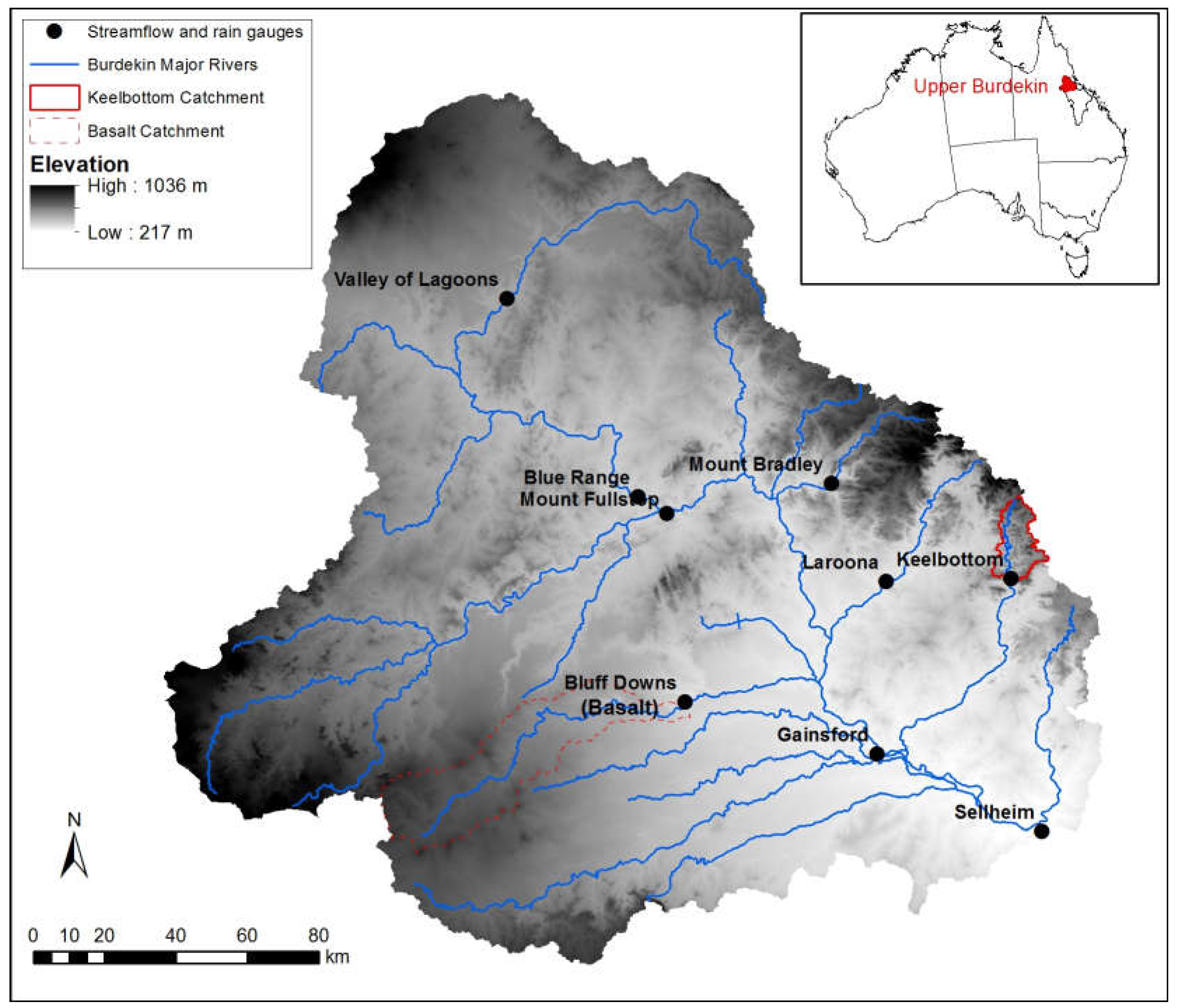
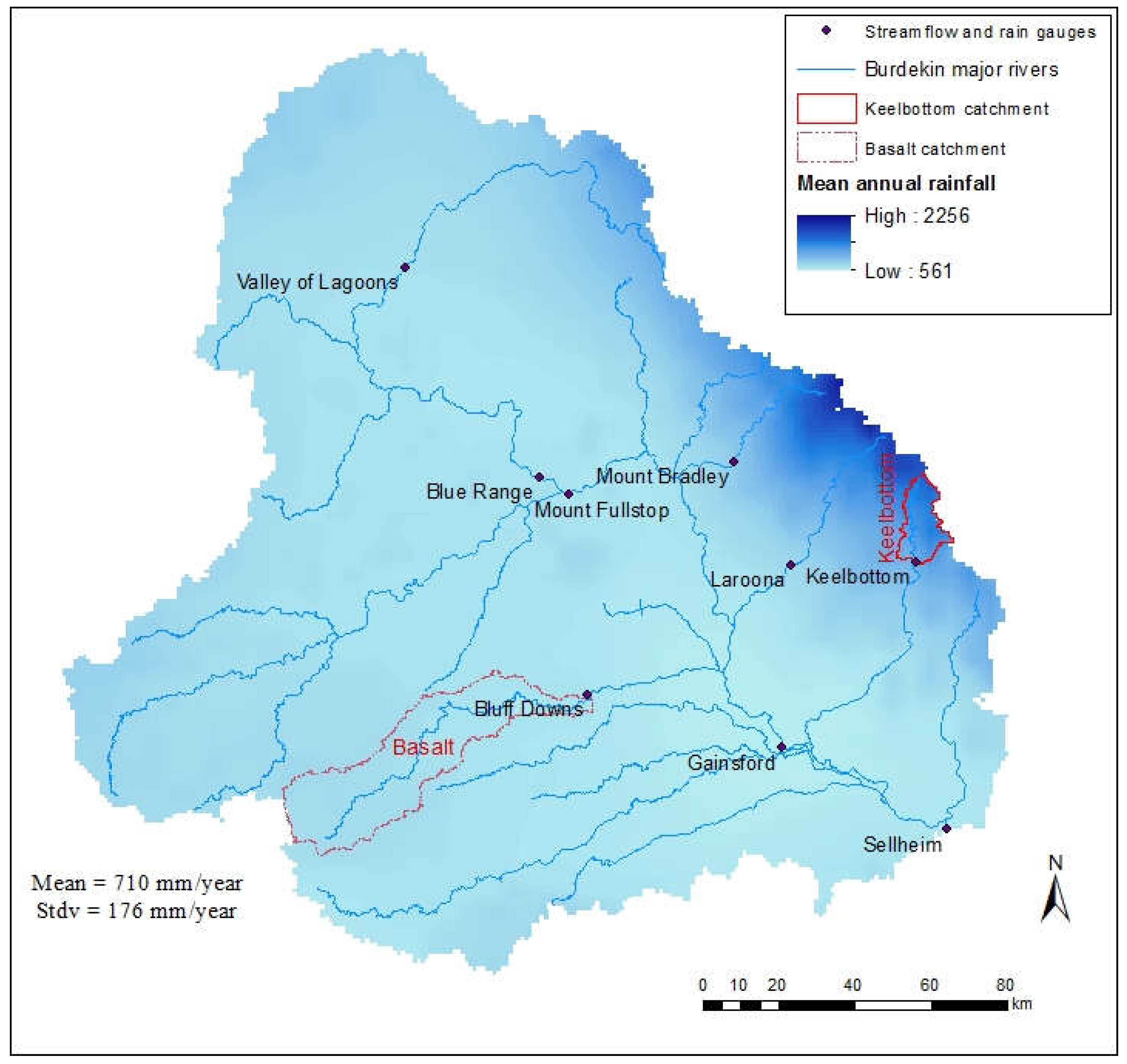
2.1. Study Site

Here we present the first assessment of long-term spatio-temporal variability of rainfall–runoff data within the Upper Burdekin—a large, dry savannah catchment in northeast Australia. We chose the Upper Burdekin catchment because it has some of the highest runoff and sediment yields of any basin draining to the GBR [34,35]. The Upper Burdekin catchment drains above Sellheim Gauging station covering 36,260 km2 (Figure 1). Elevation ranges from 217 to 1036 m a.s.l. (mean = 511 m) and average slope of the catchment is 4.85%. The catchment is largely undeveloped and is characterised by extensive eucalypt savanna woodlands [21]. Livestock grazing occupies most of the catchment (88.3%), with defence (5.5%), managed resource protection areas (3.1%), national parks (2.4%), and marsh/wetlands (0.7%) occupying the remaining areas. Vegetation cover derived from Landsat images from 2000 to 2010 show that 21.2% of the Upper Burdekin is covered by woody vegetation [36]. Soils are mostly shallow (mean depth = 0.25 m) with average depth to bedrock of 0.85 m [37]. Soils are generally weathered, sodic, and mostly red duplex soils that overlie shallow bedrock [38]. Large areas of yellow and brown spodisols are found near streams and gullies [39]. Basaltic sub-catchments in the central-west portion of the catchment have vertisol or ferrosol soils with high levels of phosphorus sourced from basalts [40]. Generally, soils have low to moderate fertility and, due to their clay surface texture and grazing pressure, surfaces are prone to crusting and hard-setting [38].
Nine telemetered stream gauging stations are nested within the Upper Burdekin operated by the Queensland Government with contributing areas ranging from 193 to 36,260 km2 and historical records ranging from 3.6 to 51.4 years (Table 1). The long term (1889–2016) mean annual precipitation within the catchment is 710 mm·y−1, which produces mean annual runoff of 131 mm·y−1 (rainfall–runoff ratio of 18%). According to Australian Water Availability Project (AWAP; [41]) data, the average annual Priestley–Taylor potential evaporation in the catchment is 1734 mm·y−1.

2.2. Materials

2.2.1. Rainfall and Streamflow Data

We used daily gridded precipitation data from Scientific Information for Land Owners (SILO; https://www.longpaddock.qld.gov.au/silo/index.html) database of the Queensland Government [42,43]. SILO is a historical climate database for Australia constructed from observational records and provides daily weather data from 1889 to present. Gridded datasets are interpolated surfaces which are stored on a regular 0.05 by 0.05° (~5 by 5 km) grid. Thirty-eight daily rain gauges in Upper Burdekin catchment were used to calculate gridded data. In addition to daily rainfall data, there are nine sub-daily recording (tipping bucket) rain gauges in the Upper Burdekin at locations adjoining Queensland Government river/stream gauges (Figure 1). Tipping buckets have variable time steps and whenever the 2 mm bucket is filled, it empties and time is recorded. Therefore the time interval is variable based on rainfall intensity.
River and stream runoff data from nine gauging stations in 15 min, hourly, daily, monthly and annual intervals are available from Department of Natural Resources and Mines (DNRM) Water Monitoring Information Portal (WMIP; https://water-monitoring.information.qld.gov.au/). Stream water levels are monitored at locations of telemetered stations and then converted to discharge by using rating curves. The rating curves are updated regularly. All data are quality checked to prevent erroneous data from being displayed. Each data record has a numerical quality code that can be seen in a downloaded data table. Moreover, all water monitoring activities are based on Department of Environment and Resource Management Monitoring and Sampling Manual, Environmental Protection (Water) Policy 2009 of Queensland Government.

2.2.2. Actual Evapotranspiration

We used MODIS satellite Global Evapotranspiration (MOD16; http://www.ntsg.umt.edu/project/mod16) datasets that are part of the NASA/EOS project to estimate global terrestrial evapotranspiration from land surfaces. MOD16 products include 8-day, monthly, and annual actual evapotranspiration (AET) and potential ET (PET) datasets in regular 1 km2 land surface grids from 2000 to 2014. The MOD16 ET datasets are estimated using the Mu et al. [44] ET algorithm that is based on the Penman-Monteith equation. MOD16 AET datasets include evaporation from wet and moist soil, from rain water intercepted by the canopy before it reaches the ground, and the transpiration through vegetation leaves and stems.

2.2.3. Ground Cover Data

We used seasonal fractional ground cover derived from USGS Landsat images (30 by 30 m resolution) by Remote Sensing Centre of the Department of Science, Information Technology and Innovation (DSITI). These data also are available through the AusCover website (http://www.auscover.org.au/xwiki/bin/view/Product+pages/Seasonal+Ground+Cover) for at least one image per standard calendar season since 1990. We also used MODIS-derived monthly vegetation fractional cover images at coarser (500 by 500 m) spatial resolution. MODIS fractional cover data represent the exposed proportion of Photosynthetic Vegetation (PV), Non-Photosynthetic Vegetation (NPV) and Bare Soil (BS) within each pixel [45]. This dataset is publically available from the Auscover website (http://www.auscover.org.au/).

2.2.4. Soil Moisture

The Soil Water Index (SWI) product of Copernicus Global Land service [46] was used to assess moisture conditions driven largely by precipitation and subsequent infiltration at various depths into the soil. The SWI was first proposed by Wagner [47] and is a method for estimating the soil moisture profile from surface observations based on only one parameter (T), which is related to infiltration time [48]. SWI data are derived from the METOP-ASCAT sensor and are available from 2007 to present in 0.1 ° (~10 by 10 km) spatial resolution for daily and 10-day temporal frequencies. SWI is available globally via the Copernicus website (http://land.copernicus.eu/global/products/swi).

3. Methods

3.1. Rainfall and Runoff Spatio-Temporal Variability

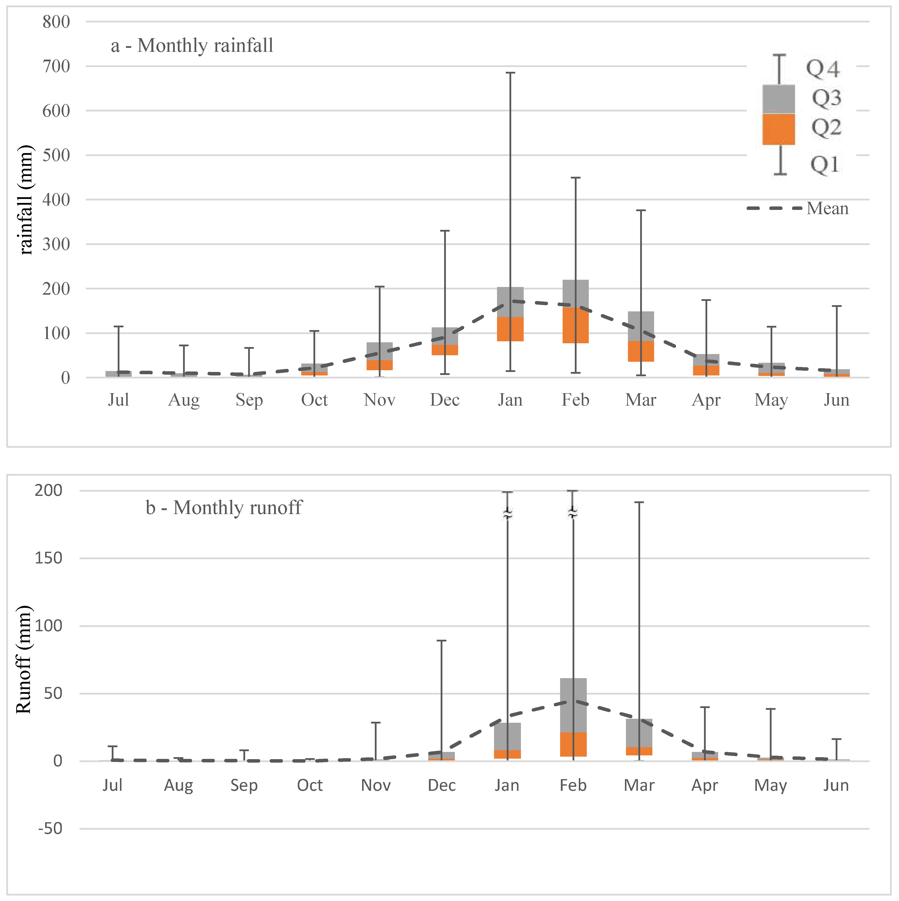
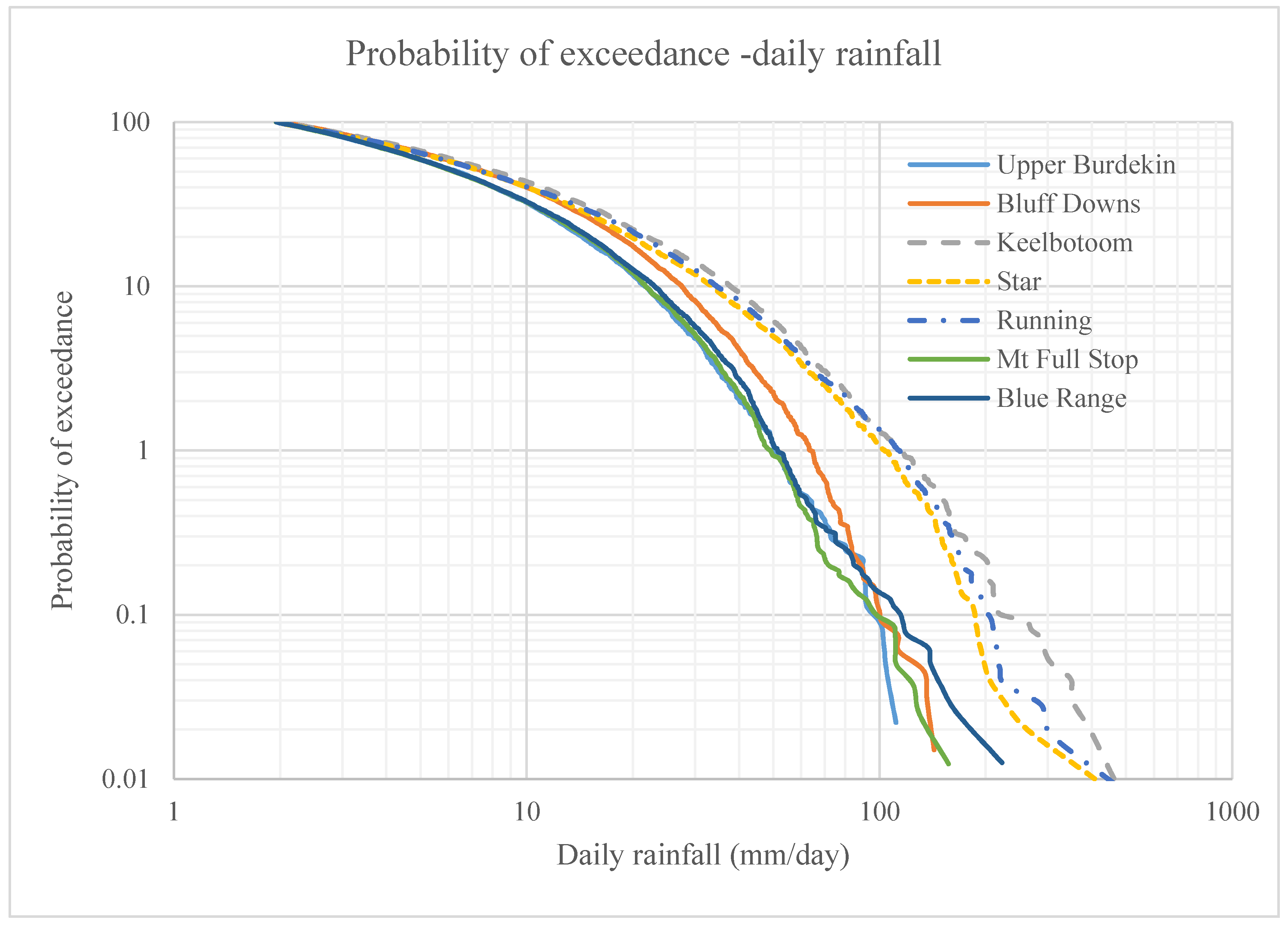
3.1.1. Variation in Rainfall Amount

We assessed long term spatial and temporal variability of rainfall in the nested catchments above the nine gauging stations (Table 1). First, SILO gridded rainfall data were clipped for each sub-catchment and spatially averaged over the catchment areas to calculate mean daily rainfall. Then monthly and annual rainfall data were calculated from daily data. The annual data analysis is based on a water year (1 July to 30 June of the next year), thus placing the Austral summer monsoonal season near the middle of the water year. Temporal variability of rainfall is calculated by using the standard deviation in each 5 km grid for all annual rainfall records.
To assess the temporal variability in rainfall, following Food and Agricultural Organization’s (FAO) protocols [49], we used the following rules to determine dry, normal, and wet weather conditions: (1) condition in a period is called dry if the rainfall received during that period has a probability of exceedance of >80%; (2) normal if it has a probability of exceedance of 20–80%; and (3) wet if it has a probability of exceedance of <20% [49]. Daily rainfall data (>2 mm·d−1) over seven catchments of Upper Burdekin were used in probability of exceedance calculations.

3.1.2. Variation in Runoff

Monthly and annual volumetric runoff ratios for each sub-catchment were calculated from accumulated rainfall and runoff for each catchment (runoff/rainfall). The effect of rainfall spatial variability on runoff was assessed by comparing runoff ratios of two sub-catchments with high (Keelbottom; 1294 mm∙y−1 on average) and low (Basalt; 664 mm∙y−1 on average) rainfall.

3.2. Changes in Land Surface Conditions

Land surface condition affects rainfall–runoff processes and alters the amount of rainfall that infiltrates and can be stored in the soil profile or runs off the catchment. The effects of ground cover and antecedent soil moisture on runoff generation were assessed using the Landsat-derived seasonal Ground Cover (GC) data of Australia to estimate the “true” ground cover for each season. GC is restricted to areas of less than 60% woody vegetation by combining information from the persistent green products and seasonal fractional cover products [50]. The GC metrics (green, non-green and bare ground) for each water year were calculated by averaging seasonal metrics. We also used MODIS-derived monthly fractional data to compare with seasonal Landsat-derived data to explore the changes in ground cover changes in monthly time periods.
To assess the effect of soil moisture on runoff generation, the SWI daily products were extracted for each catchment and then averaged into monthly and annual data. The effect of ground cover on runoff generation was evaluated by simple linear correlation between monthly ground cover and runoff ratio. To assess the relative influence of soil moisture versus ground cover on runoff, a multiple regression analysis was used. Rainfall, soil moisture, and ground cover were the independent variables in the regression analysis used to predict runoff (dependent variable) for annual time steps between water years 1990–1991 and 2015–2016. Multiple correlation coefficient and standard error statistical parameters were calculated and compared for these 26 water years. Moreover, regression analysis between annual rainfall runoff residual (P-R) vs. ground cover soil moisture was performed to determine which parameter has stronger control on runoff generation.
To eliminate the effect of rainfall variability, we compared two months (November and April) with similar long term monthly rainfalls, but with different ground cover in Upper Burdekin catchment. The hypothesis was that the slope of the linear correlation between ground cover and runoff ratio should be steeper in November than April. In other words, if ground cover and associated soil condition is important for controlling the proportion of rainfall that turns into runoff (or the runoff ratio) in these catchments, then similar rainfall in November (driest period) should produce more runoff compared to a similar event in April (wet period), as soil saturation is the controlling process. With soils in certain catchment locations being saturated in April (end of the wet season), there is more chance for precipitation becoming runoff as opposed to November (end of the dry/start of the wet season).

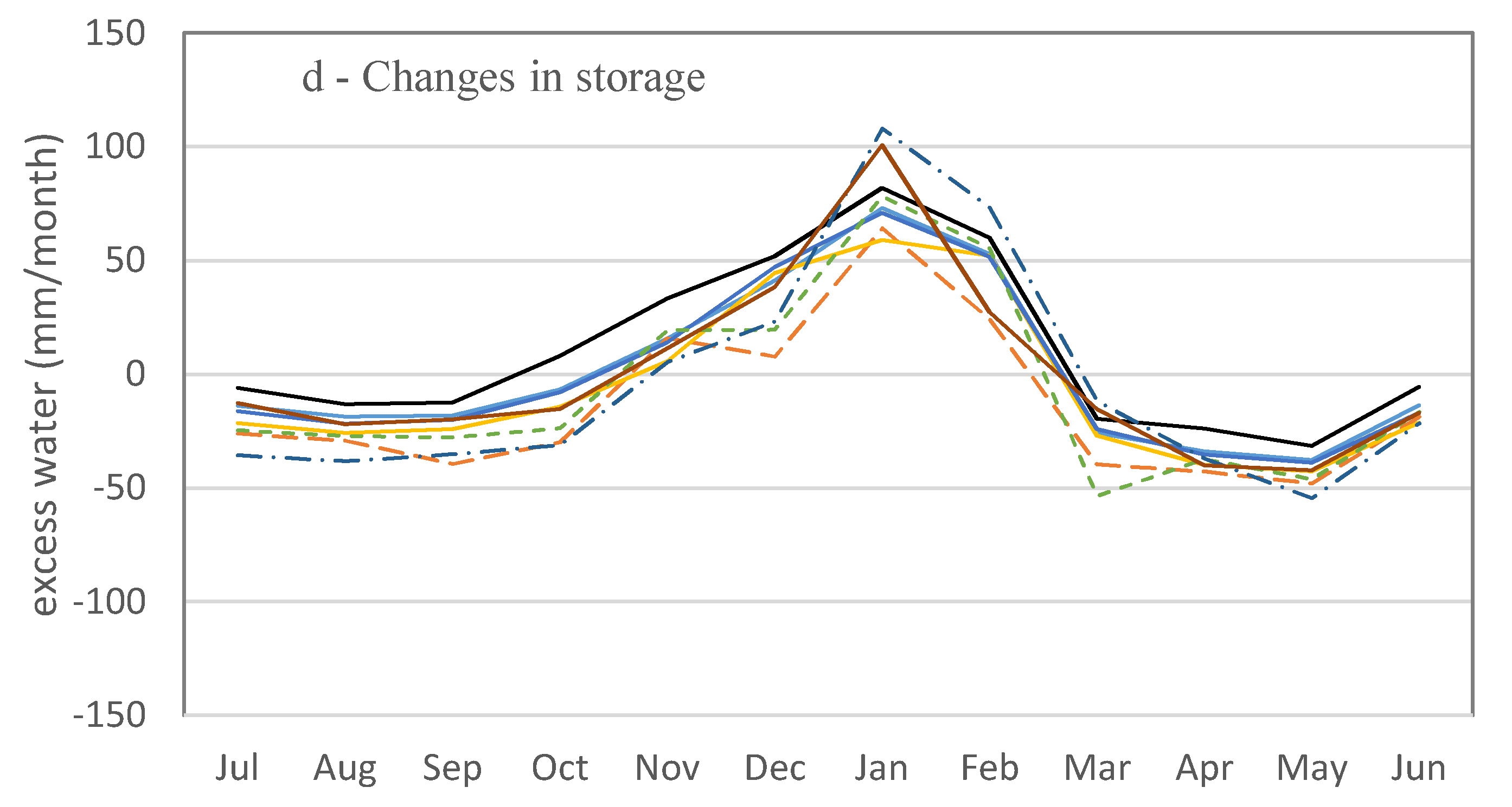
3.3. Water Balance Assessment

A water balance was used to assess how the temporal variability of rainfall affects overland flow. To estimate available water in the soil profile (S) for annual and monthly time steps, we performed a simple water balance by subtracting outputs from inputs. With no irrigation, rainfall (P) is the only input to the soil “bucket” and exfiltration from groundwater or other inputs are negligible [26]. Runoff (R) and actual evapotranspiration (AET) are the water losses from the system. Infiltration into the soil contributes to evaporation from the soil surface, transpiration by vegetation, and percolation and storage into much deeper soil layers. However, discharge into deeper groundwater is negligible for monthly and annual time intervals. Therefore, following [51], a simplified mass balance Equation (1) is used:
P t   R t A E T t = Δ S ,
where t is time period (monthly and annual in this study). We calculated the monthly and annual changes in water storage from P, R and AET parameters for all catchments for the period 2000–2014.
We also assessed the effect of number of monthly events on runoff generation. To eliminate the influence of multiple small rain events, which contribute little or no runoff, but may accumulate over long periods, several thresholds were defined in selecting events. Total event rainfall greater than various threshold values (i.e., 5, 10, 15, 20, 25, 30, 40 and 50 mm) were correlated against runoff in each catchment to determine number of the effective events.

4. Results and Discussion

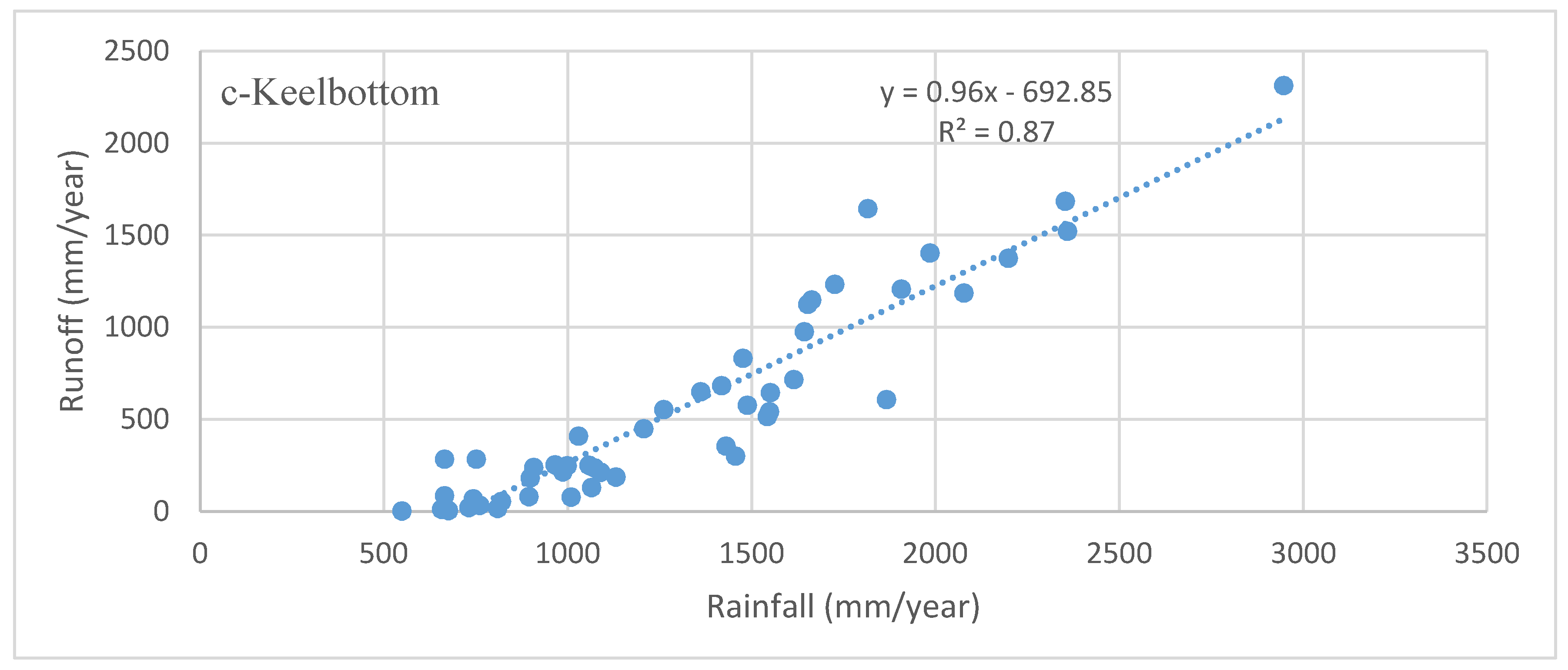
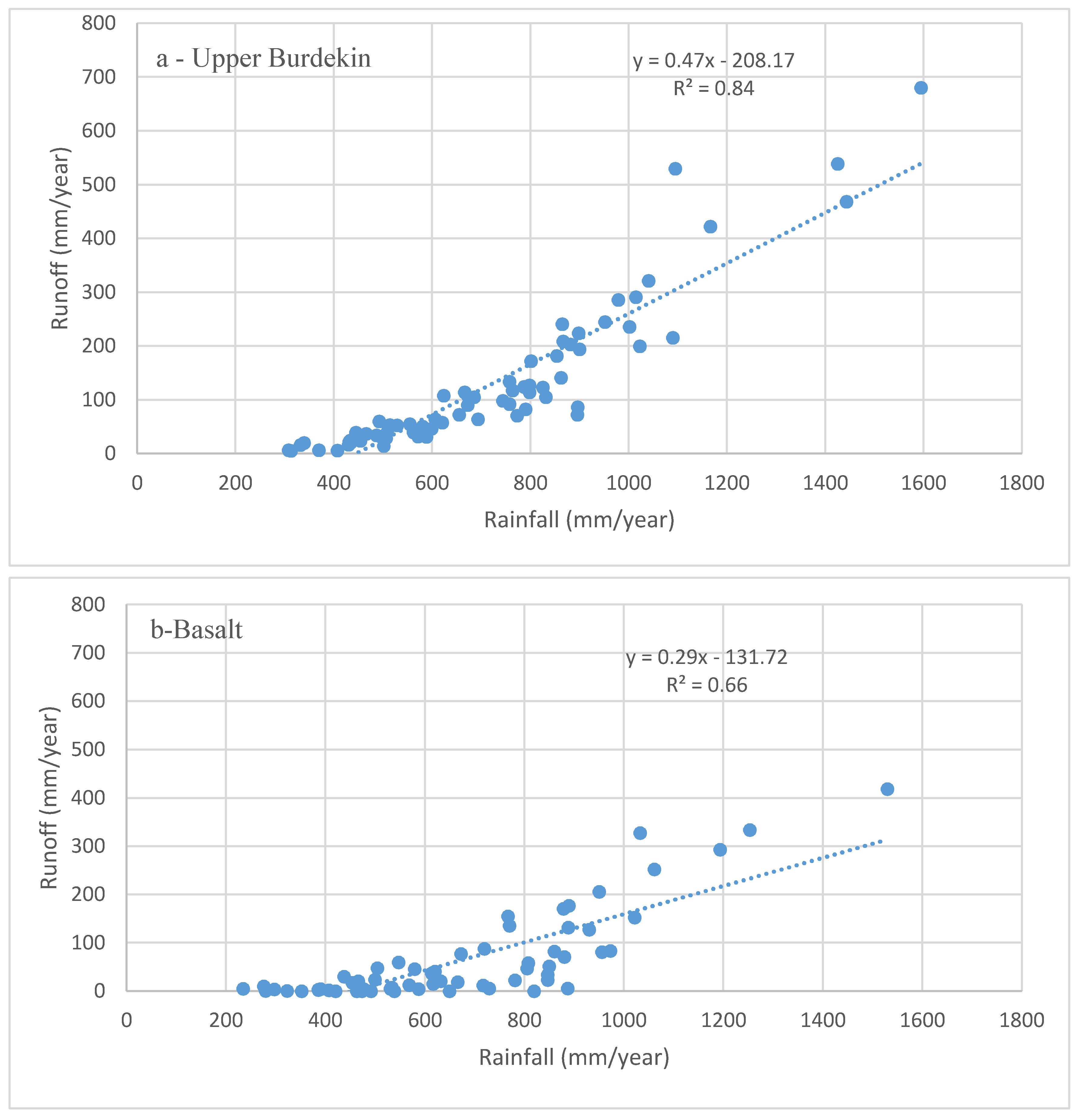
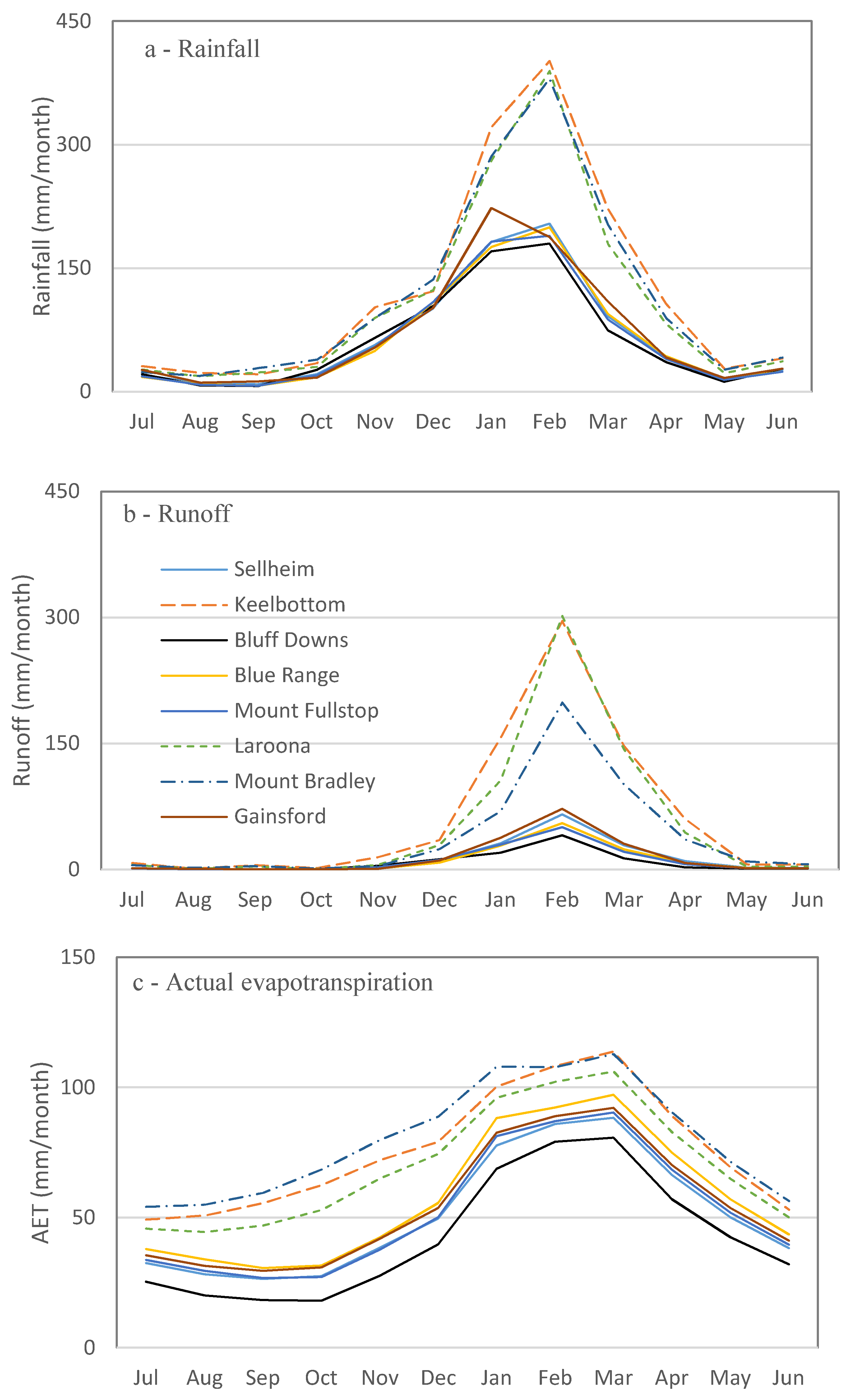
4.1. Rainfall and Runoff Spatio-Temporal Variability

4.1.1. Variation in Rainfall Amount

Throughout the Upper Burdekin catchment, long-term (1889–2016) annual rainfall varies between 560 and 2300 mm·y−1, with a mean rainfall of 710 mm·y−1 and a standard deviation of 176 mm·y−1 (Figure 2). In general, annual rainfall decreases from east to west; however, the variability of rainfall east of the Burdekin River is 10 times higher (~20 mm/linear km) than the west side of the catchment (~2 mm/km). The Upper Burdekin has experienced above average rainfall in 57 years and below average rainfall in 70 years in the last 127 years of record. Probabilities of exceedance of 20% (wet), 50% (normal), and 80% (dry) rainfall in the Upper Burdekin correspond to annual precipitation values of 895, 672, and 492 mm·y−1, respectively. A comparison of one wet (Keelbottom Creek in the east) and one dry (Basalt River in the west) sub-catchment highlight the diverse rainfall conditions within the Upper Burdekin. The Basalt sub-catchment is considerably drier (wet: 880 mm·y−1; normal: 620 mm·y−1; dry: 445 mm·y−1) than Keelbottom (wet: 1700 mm·y−1; normal: 1260 mm·y−1; dry: 825 mm·y−1).
It has been demonstrated that rainfall amount and intensity variation influence runoff generation [19,21]. However, at the catchment scale, heterogeneity in rainfall magnitude and intensity can have a significant impact on the runoff and erosion processes. By assessing temporal and spatial patterns of rainfall in multiple scales, we identified rainfall and consequently erosion hot spots. This will help government departments in targeting critical parts of catchment for land management and erosion control practices.
Temporal distribution of rainfall in the Upper Burdekin shows a typical summer dominant, monsoonal rainfall pattern for Northern Australia, with December to March being the wetter months. Ignoring the interaction between surface and groundwater and assuming that soil moisture is relatively the same at the beginning of each water year, the actual evapotranspiration of the catchment can be calculated from precipitation (710 mm·y−1) minus runoff (131 mm·y−1). Using the Budyko framework [52], low annual rainfall and actual evapotranspiration (579 mm·y−1) compared with potential evapotranspiration (~1800 mm) indicate that the Upper Burdekin catchment is categorised as a water-limited (dry) environment, although some of the wetter areas on the eastern fringes of the catchment would be classified as energy-limited (i.e., wet) environment. Therefore, this system is classified as equitant, where water-limited and energy-limited conditions are experienced on a sub-annual time-step [53]. Monthly actual evapotranspiration and runoff follow similar trends with monthly precipitation maxima in December through March. These four months contribute 74% of the annual precipitation, 89% of annual runoff, and 70% of actual evapotranspiration. This summer dominant rainfall pattern in the Upper Burdekin exhibits high inter-annual and decadal variability of rainfall, similar to rainfall variability across northern Australia and Queensland [54]. This high variability is closely linked with El Niño–Southern Oscillation (ENSO) events with above average rainfall during La Niña events and drier conditions during El Niño events [24]. Excluding minor events (<2 mm) from intensity calculations eliminates numerous small rainfalls from the analysis and more realistically reflects the correct number of storms and magnitude-intensity relationships. These larger storms are directly associated with the majority of runoff generation [19] and erosion [17].
Daily rainfall probability of exceedance (PE) (probability of the occurrence of a daily rainfall depth >2 mm) was calculated for all catchments (Figure 3). Two types of rainfall exceedance relationships can be distinguished in Figure 3. The Keelbottom, Star and Running rivers have a significantly higher probability of exceedance of rainfall than the drier catchments. The long-term (1889–2016) annual average number of rainy days (total rain >2 mm) varied over the Upper Burdekin catchment, ranging from 60 to 170 days per year with an average of 100 days per year and a standard deviation of 20 days per year. The spatial distribution of rainy days follows the same pattern as rainfall depth: higher in the east and lower in the west. The number of rainy days per annum for 1889–2016 varied from 57 to 195 days per year.

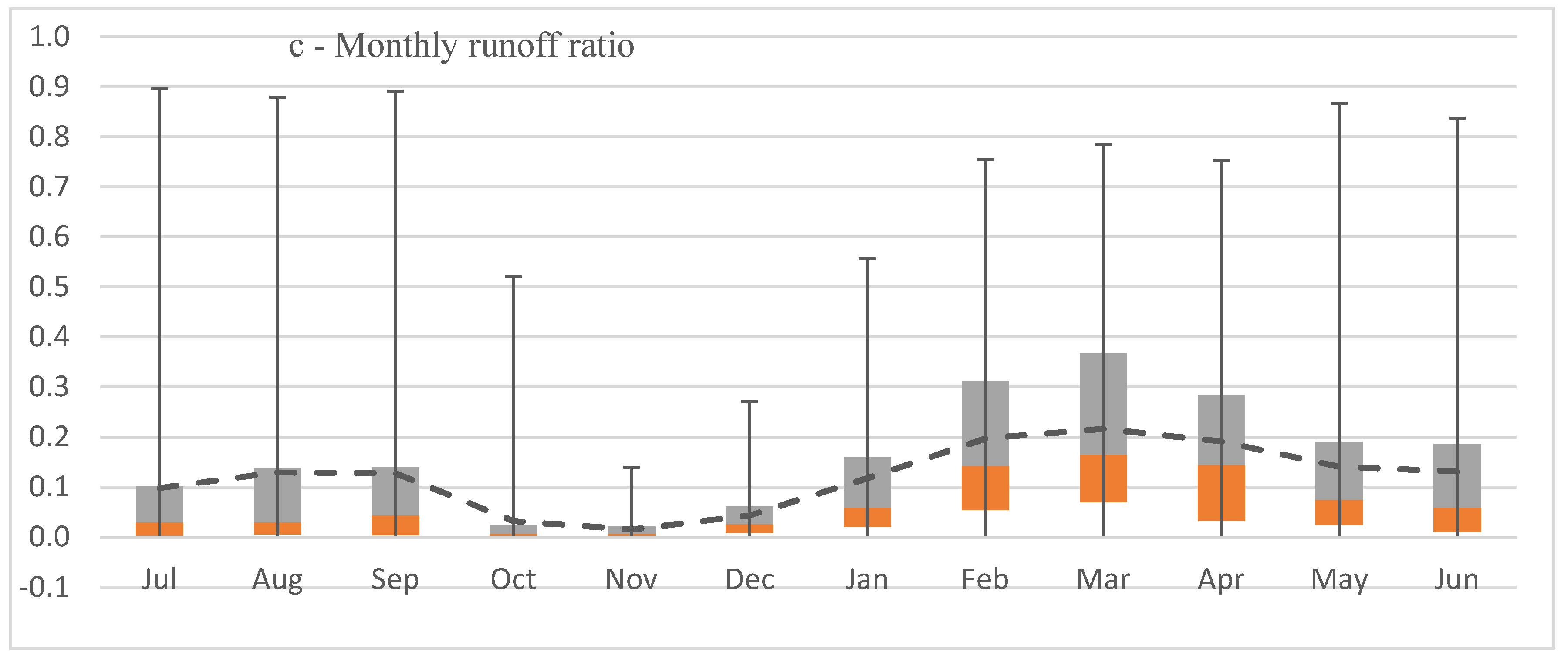
4.1.2. Runoff Variability

Runoff data for the entire Upper Burdekin catchment are available since 1948 at the Sellheim gauging station. Annual runoff varies from 5 to 680 mm·y−1 with an average of 130 mm·y−1. The annual rainfall–runoff relationship for the Upper Burdekin indicates that the annual rainfall needed to trigger runoff is ~300 mm·y−1; (Figure 4a). As in other catchments worldwide, soil characteristics (e.g., depth) and geology have significant effects on regional streamflow regime [55]. For example, the rainfall–runoff relationships for Basalt and Keelbottom catchments differ substantially. Annual rainfall required to trigger runoff in the Keelbottom catchment (with more rainfall) is higher (~550 mm) than in the Basalt catchment (~200 mm). This difference could be attributed to the greater forest cover in Keelbottom (>70%) compared to Basalt (<10%) that would buffer runoff during drier conditions together with the greater rooting depth of trees that would promote infiltration and soil water storage available for evapotranspiration [55,56]. Differences in soil depth, hydraulic conductivity, and surface geology could also play a role [31]. However, once runoff is generated, the rate of increase in discharge per unit change of rainfall is higher in the wetter (Keelbottom) catchment. The implication is that the more heavily vegetated savanna catchments require more antecedent rainfall to generate runoff than in drier, poorly vegetated catchments.
The temporal volumetric annual runoff ratio (runoff/rainfall) for the Upper Burdekin varies from 0.01 to 0.48 with an average of 0.15. Spatially, this runoff ratio is higher for humid parts of the catchment compared to dry regions. For example, the average annual runoff ratio for Keelbottom (0.01–0.91, mean = 0.35) is five-fold higher than Basalt (0.0–0.32, mean = 0.07).
The annual runoff ratio positively correlates with the magnitude of total annual rainfall (P: r = 0.88) and runoff (R: r = 0.96), and the correlation with total annual rainfall was higher (P: r = 0.89, R: r = 0.98) for above average rainfall years (wet years) than below average dry years (P: r = 0.77, R: r = 0.96). Average monthly runoff from the Upper Burdekin in the period from 1948 to 2016 ranged between 0 mm (August–October) and 45 mm (February) (Figure 5). Although January (33 mm) and February (45 mm) have higher rainfall than March (31 mm), the runoff ratio in March (0.27) is higher than January (0.12) and February (0.20) due to higher antecedent soil moisture [57,58]. Runoff ratios are low at the start of the wet season in November and increase from December to March due to increases in soil moisture. Despite low to zero rainfall from April to September, runoff ratios are also high, most likely due to carry-over soil moisture from previous months and/or lags associated with base flow generation.

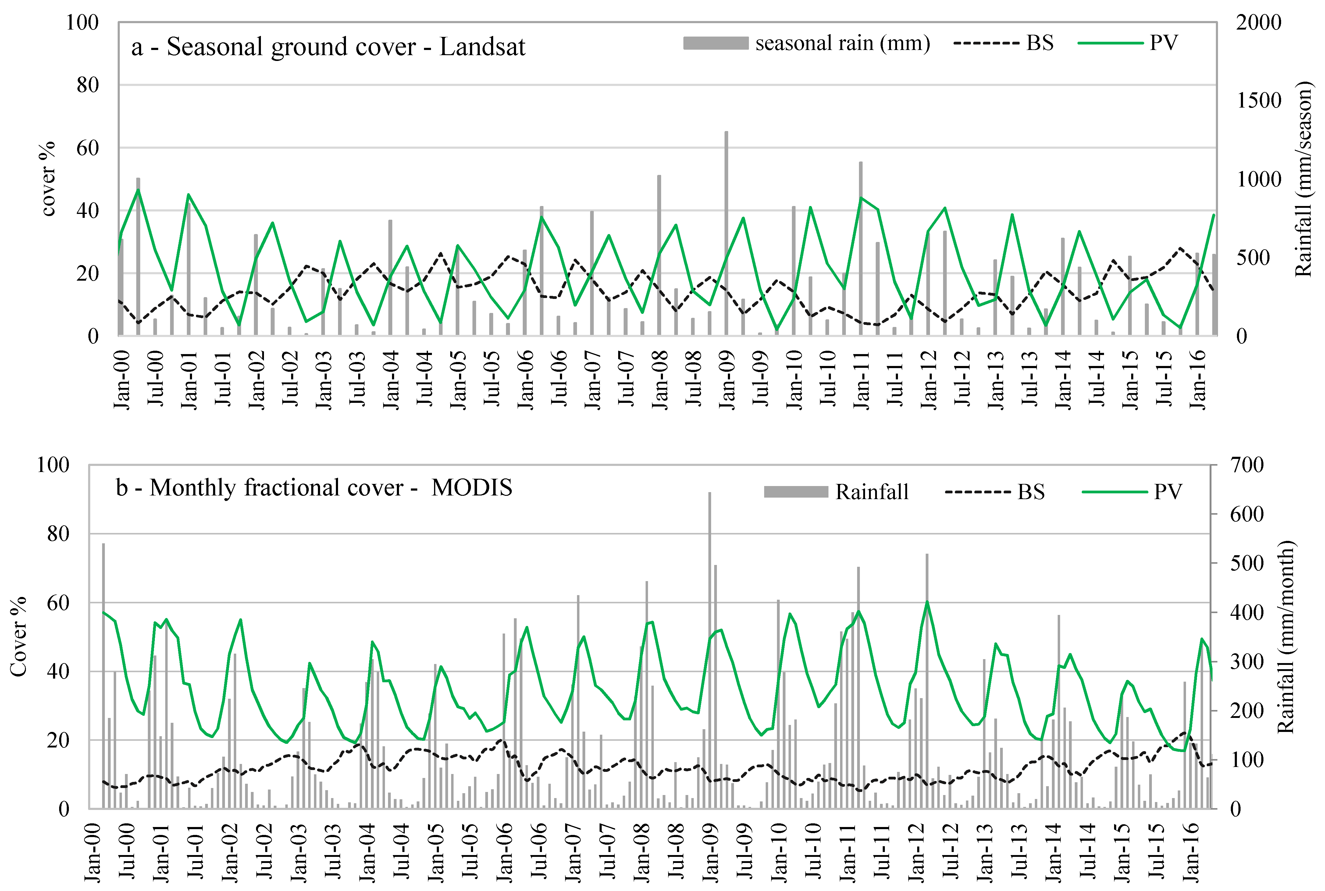
4.2. Changes in Land Surface Conditions

Seasonal ground cover data generated from Landsat and monthly fractional cover from MODIS were extracted and compared with rainfall data over the Burdekin catchment from 1990 to 2016 (Figure 6). Ground cover data consists of Photosynthetic Vegetation (PV), Non-Photosynthetic Vegetation (NPV) and Bare Soil (BS) within each pixel; the total vegetation (TVC) cover is calculated as PV + NPV. The annual total cover varies from 72% during the 1990–1995 drought to 95% in the wet period of 2010–2011, acknowledging that Landsat-derived ground cover estimates can over-predict cover by up to 20% when compared to on-ground measurements at the hillslope scale [17,59]. Seasonal green cover exhibited weak agreement with rainfall of the previous season (r = 0.5), however, the correlation of seasonal green cover with rainfall in the same season was slightly higher (r = 0.6), suggesting that seasonal periods are too long to investigate vegetation changes due to rainfall variation and are also too long to assess lag times. In contrast, monthly green cover from MODIS was weakly related with rainfall of the same month (r = 0.44), more strongly related with rainfall of the previous month (Pt−1; r = 0.69), and had the strongest relationship with total rainfall of the two previous months (Pt−2 + Pt−1; r = 0.81) across all catchments. These higher correlations highlight sub-seasonal response time of the dryland savanna systems to individual rainfall events (Figure 6).
Multiple regression analysis of annual runoff time series for the Upper Burdekin catchment showed that using only antecedent soil moisture to predict runoff was the worst option, followed by ground cover alone, and a combination of ground cover and soil moisture (Table 2). Using rainfall as the only predictor increased runoff predictions dramatically and additions of GC and SM only slightly improved further correlations (Table 2). Comparing effects of soil moisture versus ground cover on runoff revealed that for annual time steps, runoff is more sensitive to ground cover than soil moisture. Regression analysis between annual rainfall–runoff residuals (P-R) vs. ground cover and/or soil moisture, revealed that mean annual ground cover has a greater influence on the rainfall–runoff residual than soil moisture (Table 3). This might be due to very small carryover of moisture at an annual scale.
Annual soil water index (SWI) correlates positively with annual rainfall over the entire catchment (r = 0.93). Although the monthly correlation coefficient of SWI and rainfall is lower (r = 0.68) than annual, it follows a similar trend as rainfall. We used total rainfall in the prior year as a surrogate for antecedent soil moisture. The correlation analysis was performed between runoff ratio (RRt) and total rainfall of the prior year (Pt−1) and the prior two years (Pt−2 + Pt−1). There is a high correlation coefficient between runoff ratio and antecedent precipitation for both cases. Interestingly, the correlation between runoff ratio (RRt) and cumulative soil moisture of the two previous years (Pt−2 + Pt−1) was even higher (r = 0.89) than only using soil moisture for the previous year (r = 0.88). This result indicates that the persistent woody cover is responding more to these two-year deeper soil moisture stores compared to recurrent grass cover [60]. Annual RR correlates best with the maximum monthly runoff in the same year (r = 0.93).
In the Upper Burdekin, on average, ground cover in November (25% at the end of dry season) is lower than in April (50% end of wet season). Assuming ground cover influences large-scale runoff generation, we expected less runoff in April than November due to higher vegetation cover. However, results show the opposite effects with more runoff in April (10 mm) than November (3 mm) for similar size storms (>50 mm). This result can be explained by differences in antecedent soil moisture between November and April. Additional investigations of the relationship between runoff and other parameters revealed that monthly catchment runoff was highly correlated with rainfall (R vs. P: r = 0.84) followed by antecedent soil moisture (runoff versus soil moisture: r = 0.55) and ground cover (runoff versus ground cover: r = 0.55). This agrees with plot scale findings that showed that rainfall intensity had a greater influence on runoff generation than ground cover [19]. Very low correlations between runoff and antecedent soil moisture in wetter months (Table 4) could be due to the saturation of riparian areas and other hydrologically active regions of the catchment [61]. At the beginning of the wet season, low ground cover has greater influence on runoff generation (higher correlation values, Table 4), but later (in March and April), the correlations decrease as ground cover increases. This highlights the relative importance of ground cover during drier months and how runoff generation is more influenced by ground cover in drier months (when soil bucket is empty) than wetter months [19,21].
Thus, at these assessment scales (annual, seasonal and relatively large catchments), there was no significant effect of ground cover on annual runoff. In other words, fluctuations in mean annual ground cover (MODIS-derived total cover 81–91%) is not sufficient to detect changes in annual runoff. We conclude that for the full size range of catchments (193–36,260 km2), runoff generation processes are sensitive to antecedent soil moisture conditions at all scales and ground cover at finer scales, but interactions between these two parameters may occur. This highlights the complex interaction between climate and land management in rangeland environments that complicates the interpretation of data on condition and trend of ground cover [25,62,63]. Therefore, higher spatial resolution of ground cover data in shorter time periods (monthly and weekly) and at smaller scales is needed to distinguish the effects of soil surface conditions on runoff generation processes.

4.3. Water Balance Assessment

Water balance analysis showed that the average of the annual water balance from 1998 to 2014 is close to zero (+15 mm) indicating explicitly wet and dry periods in each individual year (i.e., water year starts in July with an empty bucket, then progressively fills, and then empties at the end of the water year in June). Changes in water storage at the end of the water year (July–June) are positive (Figure 7d) for years with above average annual rainfall. For example, in most (i.e., 6 of 8) of the examined catchments, the water balance was positive in 2008–2009 and 2010–2011. This carryover water is stored as soil moisture in deeper soil profiles and trees extract water from deeper in the soil to maintain transpiration in dry years [26,64,65,66]. A small amount of this water in riparian corridors of major channels may feed baseflow.
Monthly water balance analysis showed that monthly runoff, actual evapotranspiration, and water storage follow the same trend as summer rainfall (Figure 7). All the water balance elements (i.e., rainfall, runoff, water storage, and evapotranspiration) are lowest in August to October and begin to increase in November at the start of the wet season. These parameters are higher from January through March than during the rest of the year. Water storage is positive from November through February (Figure 7d), indicating that this is an energy-limited period (rainfall > runoff + evapotranspiration) and the soil “bucket” is filling with excess available water. This agrees with findings of a small-scale study in which wet season rainfall rapidly filled the soil and caused water to drain below the root-zone if the vegetation was unable to extract the water [51]. In contrast, the March to October period is water-limited with demands for evapotranspiration higher than available rain water. The water deficit in this period is supplied from water stored during the November through February wet period. Monthly runoff is at a maximum in February following the maximum monthly storage in January. Evapotranspiration is highest in March due to higher water availability in the previous two months (Figure 7c,d). There is a sharp decline in catchment water storage in March, most likely due to higher evapotranspiration because of greater vegetation cover near the end of the wet season (March) (Figure 7d). As evidence for this, monthly AET data follows the same trend as monthly green cover (r = 0.87) and peak AET (Figure 7) coincides with green cover peaks (Figure 7) in the wet season.
These monthly water analyses indicate that runoff generation in January and February is influenced by saturation overland flow due to nearly saturated soil profiles in selected portions of the catchment. These areas are probably confined to riparian corridors, swales, and areas of shallow soil, which are most likely to become saturated. Soil bucket size is also an important factor in determining soil water holding capacity. Soil depth of the Upper Burdekin catchment varies between 0.05 and 6.3 m (average 0.85 m) that indicates shallow soil bucket size and potential parts of the catchment that would most likely have saturated components. By March and continuing through October, the soil bucket starts to empty by evapotranspiration and Hortonian overland flow most likely becomes the dominant, if not exclusive, flow generation process. As also indicated by McIvor, Williams and Gardener [19], this infiltration-excess runoff is highly related to rainfall intensity in savanna rangelands.
The rainfall threshold analysis showed that for both monthly and annual time periods runoff at the catchment outlet is highly correlated with the number of storms during the wet season that exceeded 5 mm. Minor (<5 mm) rainfall events are lower than total transmission losses (infiltration, evaporation and terminal water storage) of catchments and never reach catchment outlets [67]. This finding agrees with results of Roth [21] that showed relatively high infiltration rates at the beginning of events for this area using a rainfall simulator in small plots.
Therefore, in the Upper Burdekin with high rainfall intensities and low infiltration rates, Hortonian overland flow is the dominant runoff generation mechanism, with saturation overland flow contributing somewhat to runoff during the few wet months, similar to results reported from plot studies in Australian savannas [19,21]. In contrast, subsurface flow is more common in catchments with deep soils and soils with high hydraulic conductivities and infiltration rates; in these catchments very little surface runoff is generated during very high rainfall intensities [68,69]. Our simple water balance analysis revealed that how soil moisture availability can influence HOF vs. SOF runoff generation process in savanna catchments. However, we acknowledge that this can be very uncertain and variable based on complex interactions among soils, water, and vegetation of the catchment.

5. Conclusions

Spatial and temporal rainfall variability and rainfall–runoff relationships are examined in a large savannah catchment of Queensland, Australia. Hydroclimatic parameters are highly variable in space and time. During the distinct wet and dry seasons, specific hydrological processes dominate runoff generation. The wet season occurs from November to March with higher water availability from rainfall, and consequently higher runoff, soil moisture and actual evapotranspiration. The dry season from April through October has lower rainfall and runoff, and the stored water in the soil profile is gradually depleted via evapotranspiration due to the higher vegetation cover. The soil “bucket” empties towards the end of dry season in October. It is likely that both saturation overland and Hortonian overland flow contribute to runoff generation during the wet season due to higher water availability to soil profile, while during the dry season Hortonian overland flow (infiltration-excess runoff) strongly dominates. Using seasonal Landsat-derived ground cover products at a range of spatial scales (193–36,260 km2), it is difficult to distinguish between the effects of ground cover changes and climate variability on runoff generation process. However, by using course resolution MODIS-derived monthly ground cover data, we were able to partly disentangle the effects of groundcover from soil moisture. A higher runoff–ground cover correlation in drier months with sparse cover highlighted the critical role of cover at the onset of the wet season (driest period) and how runoff generation is more sensitive to cover in drier months than in wetter months. Thus, we conclude that these effects are more clearly expressed, and changes potentially measurable, over smaller areas and time periods than the scales assessed in this paper. This type of coarse catchment-scale hydrological assessment improves our understanding of the dominant processes and drivers of runoff. We believe that such in-depth, catchment-based understanding is critical to bridge the gap between small-scale and large-scale studies, and to assist with upscaling results from data-rich plot scale studies to more applicable, broad catchment scales. Therefore, to separate ground cover and climate variability effects, we should focus on in-depth rainfall–runoff processes by using finer resolution datasets in a process-based hydrological model of smaller (<100 km2) catchments. The results of this study can be used to better understand the hydrological processes of dryland environments elsewhere in the world with similar rangeland and climate conditions and are critical to better understand the hydrological processes of dryland environments and subsequent effects of exposure of coral reef ecosystems in Australia to terrestrial runoff.

Acknowledgments

We thank Copernicus Global Land Service for providing Soil Water Index data. MOD16b Evapotranspiration data were provided by Numerical Terradynamic Simulation Group of The University of Montana. Seasonal and monthly ground cover were downloaded from Terrestrial Ecosystem Research Network, AusCover. Authors thank Queensland Government departments for providing rainfall and discharge data. Authors also would like to thank three CSIRO reviewers John Gallant, Tim McVicar and Ralph Trancoso for their helpful comments, as well as two anonymous reviewers and the Associate Editor. The authors would also like to acknowledge funding from the CSIRO and the National Environmental Science Program (NESP) Tropical Water Quality Hub.

Author Contributions

Ben Jarihani, Roy Sidle, Rebecca Bartley, Christian Roth and Scott Wilkinson designed the experiments; Ben Jarihani analysed the data and wrote the paper; and Roy Sidle, Rebecca Bartley, Christian Roth and Scott Wilkinson revised the paper.

Conflicts of Interest

The authors declare no conflict of interest.

References

  1. De’ath, G.; Fabricius, K.E.; Sweatman, H.; Puotinen, M. The 27-year decline of coral cover on the Great Barrier Reef and its causes. Proc. Natl. Acad. Sci. USA 2012, 109, 17995–17999. [Google Scholar] [CrossRef] [PubMed]
  2. Edinger, E.N.; Jompa, J.; Limmon, G.V.; Widjatmoko, W.; Risk, M.J. Reef degradation and coral biodiversity in indonesia: Effects of land-based pollution, destructive fishing practices and changes over time. Mar. Pollut. Bull. 1998, 36, 617–630. [Google Scholar] [CrossRef]
  3. Fabricius, K.; Logan, M.; Weeks, S.; Lewis, S.; Brodie, J. Changes in water clarity in response to river discharges on the Great Barrier Reef continental shelf: 2002–2013. Estuar. Coast. Shelf Sci. 2016, 173, A1–A15. [Google Scholar] [CrossRef]
  4. Richmond, R.H. Coral reefs: Present problems and future concerns resulting from anthropogenic disturbance. Am. Zool. 1993, 33, 524–536. [Google Scholar] [CrossRef]
  5. Rogers, C.S. Responses of coral reefs and reef organisms to sedimentation. Mar. Ecol. Prog. Ser. Oldend. 1990, 62, 185–202. [Google Scholar] [CrossRef]
  6. Sharples, J.; Middelburg, J.J.; Fennel, K.; Jickells, T.D. What proportion of riverine nutrients reaches the open ocean? Glob. Biogeochem. Cycles 2017, 31, 39–58. [Google Scholar] [CrossRef]
  7. Devlin, M.J.; Harkness, P.; McKinna, L.; Abbott, B.N.; Brodie, J. Exposure of riverine plume waters in the Great Barrier Reef: Mapping of exposure and risk to gbr ecosystems. Mar. Pollut. Bull. 2012, 65, 224–235. [Google Scholar] [CrossRef] [PubMed]
  8. Brodie, J.; Binney, J.; Fabricius, K.; Gordon, I.; Hoegh-Guldberg, O.; Hunter, H.M.; O’Reagain, P.; Pearson, R.; Quirk, M.; Thorburn, P.J.; et al. Synthesis of Evidence to Support the Scientific Consensus Statement on Water Quality in the Great Barrier Reef; Reef Water Quality Protection Plan Secretariat: Brisbane, Queensland, Australia, 2008. [Google Scholar]
  9. Fabricius, K.E. Effects of terrestrial runoff on the ecology of corals and coral reefs: Review and synthesis. Mar. Pollut. Bull. 2005, 50, 125–146. [Google Scholar] [CrossRef] [PubMed]
  10. Brodie, J.E.; Kroon, F.J.; Schaffelke, B.; Wolanski, E.C.; Lewis, S.E.; Devlin, M.; Bainbridge, Z.T.; Waterhouse, J.; Davis, A.M. Terrestrial pollutant runoff to the Great Barrier Reef: An update of issues, priorities and management responses. Mar. Pollut. Bull. 2012, 65, 81–100. [Google Scholar] [CrossRef] [PubMed]
  11. Larsen, M.C.; Webb, R.M. Potential effects of runoff, fluvial sediment, and nutrient discharges on the coral reefs of Puerto Rico. J. Coast. Res. 2009, 251, 189–208. [Google Scholar] [CrossRef]
  12. Access, E.D. Economic Contribution of the Great Barrier Reef; Great Barrier Reef Marine Park Authority: Townsville, Queensland, Australia, 2013.
  13. Wenger, A.S.; Johansen, J.L.; Jones, G.P. Increasing suspended sediment reduces foraging, growth and condition of a planktivorous damselfish. J. Exp. Mar. Biol. Ecol. 2012, 428, 43–48. [Google Scholar] [CrossRef]
  14. McCloskey, G.; Waters, D.; Baheerathan, R.; Darr, S.; Dougall, C.; Ellis, R.; Fentie, B.; Hateley, L. Modelling Reductions of Pollutant Loads Due to Improved Management Practices in the Great Barrier Reef Catchments: Updated Methodology and Results-Technical Report for Reef Report Card 2015; Queensland Department of Natural Resources and Mines: Brisbane, Queensland, Australia, 2017.
  15. Furnas, M. Catchments and Corals, Terrestrial Runoff to the Great Barrier Reef 2003; Australian Institute of Marine Science: Townsville, Queensland, Australia, 2002.
  16. Thorburn, P.J.; Wilkinson, S.N.; Silburn, D.M. Water quality in agricultural lands draining to the Great Barrier Reef: Causes, management and priorities. Agric. Ecosyst. Environ. 2013, 180, 4–20. [Google Scholar] [CrossRef]
  17. Bartley, R.; Roth, C.H.; Ludwig, J.; McJannet, D.; Liedloff, A.; Corfield, J.; Hawdon, A.; Abbott, B. Runoff and erosion from Australia’s tropical semi-arid rangelands: Influence of ground cover for differing space and time scales. Hydrol. Process. 2006, 20, 3317–3333. [Google Scholar] [CrossRef]
  18. Scanlan, J.C.; Pressland, A.J.; Myles, D.J. Run-off and soil movement on mid-slopes in north-east Queensland grazed woodlands. Rangel. J. 1996, 18, 33–46. [Google Scholar] [CrossRef]
  19. McIvor, J.G.; Williams, J.; Gardener, C.J. Pasture management influences runoff and soil movement in the semi-arid tropics. Aust. J. Exp. Agric. 1995, 35, 55–65. [Google Scholar] [CrossRef]
  20. Silburn, D.M.; Carroll, C.; Ciesiolka, C.A.A.; deVoil, R.C.; Burger, P. Hillslope runoff and erosion on duplex soils in grazing lands in semi-arid central Queensland. I. Influences of cover, slope, and soil. Soil Res. 2011, 49, 105–117. [Google Scholar] [CrossRef]
  21. Roth, C. A framework relating soil surface condition to infiltration and sediment and nutrient mobilisation in grazed rangelands of north-eastern Queensland. Earth Surf. Process. Landf. 2004, 29, 1093–1104. [Google Scholar] [CrossRef]
  22. Ludwig, J.A.; Bartley, R.; Hawdon, A.; Abbott, B.; McJannet, D. Patch configuration non-linearly affects sediment loss across scales in a grazed catchment in north-east Australia. Ecosystems 2007, 10, 839–845. [Google Scholar] [CrossRef]
  23. Post, D.A. Regionalizing rainfall-runoff model parameters to predict the daily streamflow of ungauged catchments in the dry tropics. Hydrol. Res. 2009, 40, 433–444. [Google Scholar] [CrossRef]
  24. Lough, J.M. Great Barrier Reef coral luminescence reveals rainfall variability over northeastern Australia since the 17th century. Paleoceanography 2011, 26, 1–14. [Google Scholar] [CrossRef]
  25. Peña-Arancibia, J.L.; van Dijk, A.I.J.M.; Guerschman, J.P.; Mulligan, M.; Bruijnzeel, L.A.; McVicar, T.R. Detecting changes in streamflow after partial woodland clearing in two large catchments in the seasonal tropics. J. Hydrol. 2012, 416–417, 60–71. [Google Scholar] [CrossRef]
  26. Leuning, R.; Cleugh, H.A.; Zegelin, S.J.; Hughes, D. Carbon and water fluxes over a temperate eucalyptus forest and a tropical wet/dry savanna in Australia: Measurements and comparison with modis remote sensing estimates. Agric. For. Meteorol. 2005, 129, 151–173. [Google Scholar] [CrossRef]
  27. Thornton, C.M.; Cowie, B.A.; Freebairn, D.M.; Playford, C.L. The brigalow catchment study: Ii. Clearing brigalow (acacia harpophylla) for cropping or pasture increases runoff. Aust. J. Soil Res. 2007, 45, 496–511. [Google Scholar] [CrossRef]
  28. Siriwardena, L.; Finlayson, B.L.; McMahon, T.A. The impact of land use change on catchment hydrology in large catchments: The comet river, central Queensland, Australia. J. Hydrol. 2006, 326, 199–214. [Google Scholar] [CrossRef]
  29. Bartley, R.; Corfield, J.P.; Hawdon, A.A.; Kinsey-Henderson, A.E.; Abbott, B.N.; Wilkinson, S.N.; Keen, R.J. Can changes to pasture management reduce runoff and sediment loss to the Great Barrier Reef? The results of a 10-year study in the Burdekin catchment, Australia. Rangel. J. 2014, 36, 67–84. [Google Scholar] [CrossRef]
  30. Wohl, E.; Barros, A.; Brunsell, N.; Chappell, N.A.; Coe, M.; Giambelluca, T.; Goldsmith, S.; Harmon, R.; Hendrickx, J.M.H.; Juvik, J.; et al. The hydrology of the humid tropics. Nat. Clim. Chang. 2012, 2, 655–662. [Google Scholar] [CrossRef]
  31. Trancoso, R.; Larsen, J.R.; McAlpine, C.; McVicar, T.R.; Phinn, S. Linking the Budyko framework and the Dunne diagram. J. Hydrol. 2016, 535, 581–597. [Google Scholar] [CrossRef]
  32. Horton, R.E. The role of infiltration in the hydrologic cycle. EOS Trans. Am. Geophys. Union 1933, 14, 446–460. [Google Scholar] [CrossRef]
  33. Dunne, T.; Black, R.D. Partial area contributions to storm runoff in a small New England watershed. Water Resour. Res. 1970, 6, 1296–1311. [Google Scholar] [CrossRef]
  34. Bartley, R.; Croke, J.; Bainbridge, Z.T.; Austin, J.M.; Kuhnert, P.M. Combining contemporary and long-term erosion rates to target erosion hot-spots in the Great Barrier Reef, Australia. Anthropocene 2015, 10, 1–12. [Google Scholar] [CrossRef]
  35. Bainbridge, Z.T.; Lewis, S.E.; Smithers, S.G.; Kuhnert, P.M.; Henderson, B.L.; Brodie, J.E. Fine-suspended sediment and water budgets for a large, seasonally dry tropical catchment: Burdekin River catchment, Queensland, Australia. Water Resour. Res. 2014, 50, 9067–9087. [Google Scholar] [CrossRef]
  36. Flood, N.; Danaher, T.; Gill, T.; Gillingham, S. An operational scheme for deriving standardised surface reflectance from landsat tm/etm+ and spot hrg imagery for eastern Australia. Remote Sens. 2013, 5, 83. [Google Scholar] [CrossRef]
  37. Rossel, R.V.; Chen, C.; Grundy, M.; Searle, R.; Clifford, D.; Campbell, P. The Australian three-dimensional soil grid: Australia’s contribution to the globalsoilmap project. Soil Res. 2015, 53, 845–864. [Google Scholar] [CrossRef]
  38. Rogers, L.; Cannon, M.; Barry, E. Land Resources of the Dalrymple Shire; Department of Natural Resources and CSIRO: Brisbane, Queensland, Australia, 1999.
  39. Bartley, R.; Hawdon, A.; Post, D.A.; Roth, C.H. A sediment budget in a grazed semi-arid catchment in the Burdekin basin, Australia. Geomorphology 2007, 87, 302–321. [Google Scholar] [CrossRef]
  40. Isbell, R. The Australian Soil Classification; CSIRO Publishing: Clayton, Victoria, Australia, 2016. [Google Scholar]
  41. Raupach, M.; Briggs, P.; Haverd, V.; King, E.; Paget, M.; Trudinger, C. Australian water availability project (awap). CSIRO Mar. Atmos. Res. Compon. Final Rep. Phase 2008, 2, 38. [Google Scholar]
  42. Jeffrey, S.J.; Carter, J.O.; Moodie, K.B.; Beswick, A.R. Using spatial interpolation to construct a comprehensive archive of Australian climate data. Environ. Model. Soft. 2001, 16, 309–330. [Google Scholar] [CrossRef]
  43. Jones, D.A.; Wang, W.; Fawcett, R. High-quality spatial climate data-sets for Australia. Aust. Meteorol. Oceanogr. J. 2009, 58, 233. [Google Scholar] [CrossRef]
  44. Mu, Q.; Zhao, M.; Running, S.W. Improvements to a modis global terrestrial evapotranspiration algorithm. Remote Sens. Environ. 2011, 115, 1781–1800. [Google Scholar] [CrossRef]
  45. Guerschman, J.P.; Scarth, P.F.; McVicar, T.R.; Renzullo, L.J.; Malthus, T.J.; Stewart, J.B.; Rickards, J.E.; Trevithick, R. Assessing the effects of site heterogeneity and soil properties when unmixing photosynthetic vegetation, non-photosynthetic vegetation and bare soil fractions from landsat and modis data. Remote Sens. Environ. 2015, 161, 12–26. [Google Scholar] [CrossRef]
  46. Copernicus Service Information. Soil Water Index. Available online: http://land.copernicus.eu/global/products/swi (accessed on 15 August 2016).
  47. Wagner, W. Soil Moisture Retrieval from ERS Scatterometer Data; Veroffentlichung des Instituts fur Photogrammetrie und Fernerkundung: Vienna, Austria, 1998. [Google Scholar]
  48. Albergel, C.; Rüdiger, C.; Pellarin, T.; Calvet, J.-C.; Fritz, N.; Froissard, F.; Suquia, D.; Petitpa, A.; Piguet, B.; Martin, E. From near-surface to root-zone soil moisture using an exponential filter: An assessment of the method based on in-situ observations and model simulations. Hydrol. Earth Syst. Sci. Discuss. 2008, 12, 1323–1337. [Google Scholar] [CrossRef]
  49. Food and Agriculture Organization of the United Nations. CROPWAT: A Computer Program for Irrigation Planning and Management; FAO Irrigation and Drainage Paper; FAO: Rome, Italy, 2009; Volume 46. [Google Scholar]
  50. Trevithick, R.; Scarth, P.; Tindall, D.; Denham, R.; Flood, N. Cover under Trees: Rp64g Synthesis Report; Department of Science, Information Technology, Innovation and the Arts: Brisbane, Queensland, Australia, 2014.
  51. Williams, J.; Bui, E.N.; Gardner, E.A.; Littleboy, M.; Probert, M.E. Tree clearing and dryland salinity hazard in the upper Burdekin catchment of north Queensland. Aust. J. Soil Res. 1997, 35, 785–801. [Google Scholar] [CrossRef]
  52. Budyko, M. Climate and Life; Academic Press: New York, NY, USA, 1974. [Google Scholar]
  53. McVicar, T.R.; Roderick, M.L.; Donohue, R.J.; Van Niel, T.G. Less bluster ahead? Ecohydrological implications of global trends of terrestrial near-surface wind speeds. Ecohydrology 2012, 5, 381–388. [Google Scholar] [CrossRef]
  54. Petheram, C.; McMahon, T.A.; Peel, M.C. Flow characteristics of rivers in northern Australia: Implications for development. J. Hydrol. 2008, 357, 93–111. [Google Scholar] [CrossRef]
  55. Trancoso, R.; Phinn, S.; McVicar, T.R.; Larsen, J.R.; McAlpine, C.A. Regional variation in streamflow drivers across a continental climatic gradient. Ecohydrology 2017, 10, e1816. [Google Scholar] [CrossRef]
  56. Yang, Y.; Donohue, R.J.; McVicar, T.R. Global estimation of effective plant rooting depth: Implications for hydrological modeling. Water Resour. Res. 2016, 52, 8260–8276. [Google Scholar] [CrossRef]
  57. Sidle, R.C.; Tsuboyama, Y.; Noguchi, S.; Hosoda, I.; Fujieda, M.; Shimizu, T. Seasonal hydrologic response at various spatial scales in a small forested catchment, Hitachi Ohta, Japan. J. Hydrol. 1995, 168, 227–250. [Google Scholar] [CrossRef]
  58. Tsuboyama, Y.; Sidle, R.C.; Noguchi, S.; Murakami, S.; Shimizu, T. A zero-order basin—Its contribution to catchment hydrology and internal hydrological processes. Hydrol. Process. 2000, 14, 387–401. [Google Scholar] [CrossRef]
  59. Wilkinson, S.N.; Dougall, C.; Kinsey-Henderson, A.E.; Searle, R.; Ellis, R.; Bartley, R. Development of a time-stepping sediment budget model for assessing land use impacts in large river basins. Sci. Total Environ. 2014, 468–469, 1210–1224. [Google Scholar] [CrossRef] [PubMed]
  60. Donohue, R.J.; McVicar, T.R.; Roderick, M.L. Climate-related trends in Australian vegetation cover as inferred from satellite observations, 1981–2006. Glob. Chang. Biol. 2009, 15, 1025–1039. [Google Scholar] [CrossRef]
  61. McDonnell, J.J. Where does water go when it rains? Moving beyond the variable source area concept of rainfall-runoff response. Hydrol. Process. 2003, 17, 1869–1875. [Google Scholar] [CrossRef]
  62. Bastin, G.; Scarth, P.; Chewings, V.; Sparrow, A.; Denham, R.; Schmidt, M.; O’Reagain, P.; Shepherd, R.; Abbott, B. Separating grazing and rainfall effects at regional scale using remote sensing imagery: A dynamic reference-cover method. Remote Sens. Environ. 2012, 121, 443–457. [Google Scholar] [CrossRef]
  63. Scarth, P.; Röder, A.; Schmidt, M.; Denham, R. Tracking Grazing Pressure and Climate Interaction—The Role of Landsat Fractional Cover in Time Series Analysis. In Proceedings of the 15th Australasian Remote Sensing and Photogrammetry Conference, Alice Springs, Australia, 13–16 September 2010; pp. 13–17. [Google Scholar]
  64. Beringer, J.; Hutley, L.B.; Hacker, J.M.; Neininger, B.; Paw U, K.T. Patterns and processes of carbon, water and energy cycles across northern Australian landscapes: From point to region. Agric. For. Meteorol. 2011, 151, 1409–1416. [Google Scholar] [CrossRef]
  65. Cernusak, L.A.; Hutley, L.B.; Beringer, J.; Holtum, J.A.M.; Turner, B.L. Photosynthetic physiology of eucalypts along a sub-continental rainfall gradient in northern Australia. Agric. For. Meteorol. 2011, 151, 1462–1470. [Google Scholar] [CrossRef]
  66. Hutley, L.B.; Beringer, J.; Isaac, P.R.; Hacker, J.M.; Cernusak, L.A. A sub-continental scale living laboratory: Spatial patterns of savanna vegetation over a rainfall gradient in northern Australia. Agric. For. Meteorol. 2011, 151, 1417–1428. [Google Scholar] [CrossRef]
  67. Jarihani, A.A.; Larsen, J.R.; Callow, J.N.; McVicar, T.R.; Johansen, K. Where does all the water go? Partitioning water transmission losses in a data-sparse, multi-channel and low-gradient dryland river system using modelling and remote sensing. J. Hydrol. 2015, 529, 1511–1529. [Google Scholar] [CrossRef]
  68. Lane, P.N.J.; Croke, J.C.; Dignan, P. Runoff generation from logged and burnt convergent hillslopes: Rainfall simulation and modelling. Hydrol. Process. 2004, 18, 879–892. [Google Scholar] [CrossRef]
  69. Sarkar, R.; Dutta, S.; Dubey, A.K. An insight into the runoff generation processes in wet sub-tropics: Field evidences from a vegetated hillslope plot. CATENA 2015, 128, 31–43. [Google Scholar] [CrossRef]
Figure 1. Study site location and rainfall/discharge gauging sites location. The inset map shows the Upper Burdekin basin highlighted in red within the Burdekin River basin.
Water 09 00540 g001
Figure 2. Distribution of long term (1889–2016) annual rainfall of Upper Burdekin catchment. This map is based on daily gridded 5 × 5 km rainfall data from SILO.
Water 09 00540 g002
Figure 3. Temporal distribution of the rainfall in Upper Burdekin. Probability of exceedance for daily rainfall data (>2 mm) over seven catchments of Upper Burdekin. Gainsford and Valley of Lagoons catchments are excluded due to shorter data records. Wet (eastern) catchments are presented in dashed-line and drier (western) catchments have continuous lines.
Water 09 00540 g003
Figure 4. Annual rainfall–runoff relations in Upper Burdekin catchment above Sellheim (a); Basalt (b) and Keelbottom (c) gauge stations for the period of 1948–2016.
Water 09 00540 g004aWater 09 00540 g004b
Figure 5. Distribution of monthly rainfall (a); runoff (b) and runoff ratio (c) in Upper Burdekin. Monthly analysis is based on data records at Sellheim gauging station 1948–2016.
Water 09 00540 g005aWater 09 00540 g005b
Figure 6. (a) Seasonal and monthly ground cover changes in the Upper Burdekin. Part a—Seasonal Bare Soil (BS) of Photosynthetic Vegetation (PV) cover from Department of Science, Information Technology and Innovation remote sensing group ground cover data [50] from 2000 to 2016. Summer: December to February; Autumn: March to May; Winter: June to August; and Spring: September to November; (b) Monthly fractional cover extracted from MODIS datasets [45] during 2000–2016.
Water 09 00540 g006
Figure 7. Monthly water balance calculations for catchments based on rainfall (a); runoff (b) and evapotranspiration (c) during 2000 to 2014, except for Gainsford that started in 2004. Changes in water storage (d) are calculated based on Equation (1) by subtracting runoff and evapotranspiration from rainfall data for each month.
Water 09 00540 g007aWater 09 00540 g007b
Table 1. Characteristics of the currently operational stream gauging stations in the Upper Burdekin Catchment.
Site NameSite No.River NameLatitudeLongitudeSite CommencedData Period (year)Catchment Area (km2)Mean Annual Rainfall (mm·y−1)Mean Annual PET (mm·y−1)Mean Runoff Ratio %
Sellheim120002CBurdekin20.01° S146.44° E1 October 196847.736,260707174815
Keelbottom120102AKeelbottom19.37° S146.36° E23 August 196748.81931294171335
Bluff Downs120106BBasalt19.68° S145.54° E1 October 196748.7128366417308
Blue Range120107BBurdekin19.16° S145.42° E1 October 198233.710,530698173812
Mount Fullstop120110ABurdekin19.21° S145.50° E16 January 196551.417,310688174011
Laroona120112AStar19.38° S146.05° E1 October 196748.712121172175730
Mount Bradley120120ARunning19.13° S145.91° E12 March 197541.34901306168628
Gainsford120122ABurdekin19.81° S146.02° E3 June 200412.026,320721174415
Valley of Lagoons120123ABurdekin18.66° S145.09° E23 October 20123.6350976617548
Table 2. Statistical parameters of multilinear regression analysis of runoff (R) vs. rainfall (P), ground cover (GC) and soil moisture (SM). Correlation increases from left to right. Sample size is 26.
ParameterR vs. SMR vs. GCR vs. GC&SMGC vs. SMR vs. PR vs. P&SMR vs. P&GCR vs. P&GC&SM
Multiple R0.340.440.450.870.900.900.910.93
Adjusted R20.080.160.130.750.800.790.810.85
Standard Error148.6141.87144.22252.0968.6570.0866.9960.90
p-ValueIntercept: 0.813Intercept: 0.050Intercept: 0.125Intercept: 0.000Intercept: 0.000Intercept: 0.001Intercept: 0.548Intercept: 0.027
SM:0.090GC:0.025GC:0.130SM:0.000P:0.000P:0.000P:0.000P:0.000
SM:0.640 SM:0.866GC:0.151GC:0.008
SM:0.025
Table 3. Statistical parameters of multilinear regression analysis of rainfall–runoff residuals (P-R) versus ground cover (GC) and soil moisture (SM). Sample size is 26.
ParameterP-R vs. SMP-R vs. GCP-R vs. GC&SM
Multiple R0.380.650.75
Adjusted R20.110.390.52
Standard Error172.54142.09125.97
p-ValueIntercept: 0.002Intercept: 0.012Intercept: 0.001
SM: 0.057GC: 0.000GC: 0.000
SM: 0.012
Table 4. Correlation coefficients (n = 312) between monthly runoff and three parameters: rainfall, antecedent soil moisture and ground cover. Total rainfall of two previous months is used as an indicator of soil moisture. Gainsford and Valley of Lagoons are excluded due to shorter data records.
ParameterRainfall–RunoffSoil Moisture–RunoffGround Cover–Runoff
MonthNov.Dec.Jan.Feb.Mar.Apr.Nov.Dec.Jan.Feb.Mar.Apr.Nov.Dec.Jan.Feb.Mar.Apr.
Upper Burdekin0.750.920.820.810.880.730.670.780.550.720.100.470.700.760.640.480.580.57
Keelbottom0.810.910.760.850.930.930.770.660.100.610.000.330.540.620.220.450.170.33
Basalt0.840.910.820.740.810.490.870.650.460.530.100.280.830.710.530.390.540.50
Blue Range0.760.910.800.790.820.850.710.850.560.700.000.240.690.790.540.350.370.42
Mount Fullstop0.770.910.840.770.870.810.750.860.570.700.000.300.730.800.570.360.480.51
Laroona0.770.920.820.890.960.890.580.600.200.700.100.350.630.560.390.530.470.50
Mount Bradley0.760.930.890.840.960.830.570.660.200.740.170.280.660.550.460.570.370.33
Average0.780.920.820.810.890.800.710.730.420.680.100.330.690.690.490.460.450.46

