Numerical Simulation of Hydrodynamics and Reaeration over a Stepped Spillway by the SPH Method


1
State Key Laboratory of Hydraulics and Mountain River Engineering, Sichuan University, Chengdu 610065, China
2
Department of Civil, Construction and Environmental Engineering, University of Napoli Federico II, Napoli 80125, Italy
3
College of Civil Engineering, Guizhou University, Guiyang 550025, China
*
Author to whom correspondence should be addressed.
Water 2017, 9(8), 565; https://doi.org/10.3390/w9080565
Submission received: 29 June 2017
/
Revised: 18 July 2017
/
Accepted: 20 July 2017
/
Published: 27 July 2017
Abstract
:Aerated flows are characterized by complex hydrodynamics and mass-transfer processes. As a Lagrangian method, smoothed particle hydrodynamics (SPH) has a significant advantage in tracking the air-water interface in turbulent flows. This paper presents the application of an SPH method to investigate hydrodynamics and reaeration over stepped spillways. In the SPH method, the entrainment of dissolved oxygen (DO) is studied using a multiphase mass transfer SPH method for reaeration. The numerical results are compared with the hydrodynamics data from Chanson and DO data from Cheng. The simulation results show that velocity distribution and the location of free-surface aeration inception agree with the experimental results. Compared with the experimental results, the distribution of DO concentration over the stepped spillway is consistent with the measurement results. The study shows that the two-phase DO mass transfer SPH model is reliable and reasonable for simulating the hydrodynamics characteristics and reaeration process.
1. Introduction
Predicting the aeration process has great significance for assessing the dissolved oxygen (DO) concentration, which is critical for the self-purification of polluted water [1]. An accurate understanding of the reaeration process plays an important role in the predicting and improving the DO content in a water body. The stepped spillway, as a type of important hydraulic structure, exhibits the dual functions of energy dissipation and the reaeration process. Research on the stepped spillway has important theoretical and applied value in hydraulic engineering and environmental hydraulics.
1.1. Previous Research on the Stepped Spillway
The stepped spillway, which has dual functions of energy dissipation and reaeration, has been used for many years. The initial application of the stepped spillway was limited to overflow energy dissipation [2,3]. Later, researchers studied the hydraulic properties and air entrainment characteristics of the stepped spillway [4,5]. However, few researchers paid attention to the mass transfer process between air and water over the spillway, until such analyses were conducted by Moog [6], and experiments were conducted by Cheng [7,8]). Considering the high turbulence and strong aeration on the spillway surface, it is difficult to accurately measure the air concentration, velocity, and dissolved gas concentration by using experimental methods, especially when the flow depth is too shallow. Some numerical methods based on the Euler grid were developed to simulate the complicated hydrodynamics, air entrainments, and mass transfer characteristics over the stepped spillway [7,8,9]. For the Euler method, the volume fraction near the interface grid is not connective and has strong discontinuities, which leads to parametric oscillation. Therefore, the validity of numerical simulation based on the Euler grid method is challenged by the large deformations of free surface and violent breakup between the interface.
Due to the inherent characteristics of the Euler method, the reaeration process that accompanies the violent interactions between the air-water interface does not show good consistency with the experimental result and full traceability of the individual particles. Accordingly, new numerical methods beyond the mesh-based method should be explored to improve the simulation accuracy for violent flows.
1.2. Smooth Particle Hydrodynamics Method
As one type of Lagrangian meshless method, the smoothed particle hydrodynamics (SPH) method has various advantages when considering large deformations and breaking flows [10,11]. To date, different SPH models have been widely studied and applied in the field of fluid mechanics. Recently, SPH methods have been widely applied in single-phase flows [12,13,14,15], multiphase flows [16,17,18], and diffusion processes between different density flows [19,20]. Compared to the Euler method, the existing Lagrangian SPH method has performed well in simulating the motion characteristic of particles. Research on mass transfer between different phases (especially the gas dissolution and mass transfer process), however, is still lacking. Hence, to extend the application of the SPH method, a multiphase mass transfer SPH model for reaeration needs to be studied. For diffusion processes with the SPH method, some studies have been reported. Cleary and Monaghan [21] adopted the SPH method to simulate heat conduction. Tartakovsky et al. [19] developed an SPH model to simulate the diffusion process with a small density difference in mineral precipitation. Aristodemo et al. [20] proposed a model to simulate the convective diffusion of soluble pollutants in water with a density ratio ranging from 0.1 to 1. All of these previous studies focused on diffusion processes through molecular diffusion between liquids. No studies based on the SPH model have been developed to investigate the mass transfer processes between different phases with air and water driven by transportation, turbulent diffusion, and other reactions.
2. SPH Model for Reaeration
The main features of the SPH method were described by Monaghan [22,23,24] and Liu et al. [25]. Details of the numerical model and discretization of the equations are described below. In the SPH method, the Function A (scalar, vector or tensor) at a certain point can be defined:
where , are positions; is the support domain; and h is the characteristic length that is called the smoothing length and calculated by ( is the dimensionless coefficient, is the particle distance). is the kernel function and should satisfy several conditions, such as compact support, positivity, monotonically decreasing with increasing distance, and the Dirac function property. The kernel function used in this paper is the Wendland kernel function [22].
Function A in Equation (1) can be approximated by using a certain number of particles with initial physical states at different positions [22]:
where j is a neighboring particle of particle i, is the mass of particle j, is the density of particle j (j = 1, 2, …, N), and N is the number of particles in the support domain . In this paper, the support domain is 2h.
Considering the derivative of the kernel function, the gradient of function A can be written as:
where is the derivative of the kernel function W and the equation can be simplified as .
2.1. Hydrodynamic Equations
The SPH form of the continuity equation is described by Monaghan [22]:
where the variable is the particle velocity at the current position.
Following Colagrossi et al. [16], the momentum equations can be discretized as air and water phases separately in the two-phase flow.
The SPH form of momentum equation (water phase) is:
The SPH form of momentum equation (air phase) is:
The Lagrange acceleration is on the left and, on the right, the first term p is the influence of pressure for acceleration, is the dissipation item, g is the body force, and is the cohesive force, for the water phase = 0.
The SPH method is used to handle the problems of initially low or no dissipation. In SPH theory, Monaghan [22] proposed artificial viscosity , which has been widely used. This not only converts kinetic energy into heat energy, providing the necessary dissipation for the shockwave, but also prevents non-physical penetration of particles for different phases. In this paper, artificial viscosity is used to solve Equations (5) and (6):
Variables , , and in Equation (7) can be rewritten as follows:
where is related to volume viscosity; the term related to can prevent particle penetration under the condition of high Mach number; ranges from 0.01 to 0.1 [20]; and , ; is the sound velocity, which can be calculated by the state equation; and , which can prevent the divergence of numbers when the particles are too close.
The XSPH method proposed by Monaghan [26] is used to correct the particle motion to ensure a more ordered flow and prevent physical penetration when the particles come closer together:
where is a specific parameter ranging from 0 to 1.0; and 0.3 is adopted in this paper.
Following Monaghan [23], the particle pressure is unique and determined by the density value through a modified Tait’s state equation [22]:
where B is the reference pressure and is the background pressure. Here, . and are the initial density for water and air, respectively. is the isentropic expansion coefficient (, ). The subscript a is for the air phase; the subscript w is for the water phase. The assumed “reference pressure B” is used to solve the pressure field distribution and ensure both the compressibility of the flow field and the uniformity of particle distribution. In the initial conditions, can be calculated as follow [27]:
where Uwmax is the maximum field velocity of the water phase and Lw is the water depth of flow field. Mach number is less than 0.1; here, it is .
For Equation (10), is the cohesion coefficient; this represents the cohesion of the same type of particles and is set to 0 for the water phase. The term can prevent air phase diffusion and broken interfaces. As suggested by Nugent et al. [28], Equation (6) can be transformed into:
2.2. The Advection-Diffusion Equation for DO
The advection-diffusion equation for DO is introduced into the model based on two-phase hydrodynamic equations:
where C is the concentration of DO, is the source term of DO, is the molecular diffusion coefficient, is the turbulent diffusion coefficient, and is the Schmidt number. A different is adopted to conduct the simulation for the two-phase flows. In this paper, is set to 1.0 [29]. Equation (13) is discretized using the SPH operator in the following section.
(1) SPH Discretization for the Diffusion Term
Similar to the heat conduction equation proposed by Cleary et al. [21], the heat transfer coefficient is replaced with the diffusion coefficient to simulate the concentration of DO. To simplify the diffusion equation, the diffusion coefficient can be defined as:
Following the method developed by Aristodemo et al. [20], the diffusion equation can be discretized into the following form:
(2) SPH Discretization for the Convection Term
The SPH operator is used to discrete the convection term:
In Equation (16), the interface is not stable when the density ratio is less than 0.1. The replacement of with is suggested to prevent strong density gradients specifically at the fluid interface [20].
(3) SPH Discretization for the Source Term
The complicated surface structure of the stepped spillway can cause collisions between the water and step, which can entrain the surrounding air in the turbulent flows to form dissolved oxygen. With the SPH method, when the water particle contacts air particles, both the contact area between the air and water and the bubble pressure will increase. As a result, the mass transfer between air and water will also increase. By referencing the classical mass transfer theory, the source term based on the SPH method can be expressed as follows:
where K is the reaeration coefficient; is the specific surface area of bubbles in the unit volume water within a search radius ; Cs is the saturated dissolved oxygen concentration under the atmospheric pressure; and C is the dissolved oxygen concentration in water. According to the mass transfer theory, when there is no air particle in the search radius, the mass transfer calculation is not conducted. Instead, the mass transfer will be conducted. For simplification, assuming that the bubble diameter is consistent in the mixing flow, the specific surface area of the bubble in unit water volume can be expressed as:
where is the number of air particles in the search radius; is the surface area of a single bubble; and is the volume of the water. On two-dimensional numerical simulation, the variables can be rewritten as follows:
According to the relationship between the dissolved gas mass transfer coefficient and the Reynolds number proposed by Banerjee et al. [30], the reaeration coefficient K can be calculated using:
where is recommended as 0.2 and is a constant value; Re is the effective Reynolds number using the formula proposed by Price [31].
2.3. Time Integration
To integrate the scheme forward in time, the Verlet explicit scheme is used [32]. Under the Courant Friedrichs Levy (CFL) condition, the unit mass force and diffusion condition derived from the viscous term are used to determine the variable time step. Detailed steps are described here.
As suggested by Monaghan [22], the time step, Δt, of unit mass force can be described as:
where fi is the acceleration of the unit mass force.
Computation of the standard time step integrates the viscosity and unit mass force effect:
where CCFL is between 0.1 and 0.2. In the paper, CCFL is set equal to 0.2.
3. Model Framework and Simulation Method
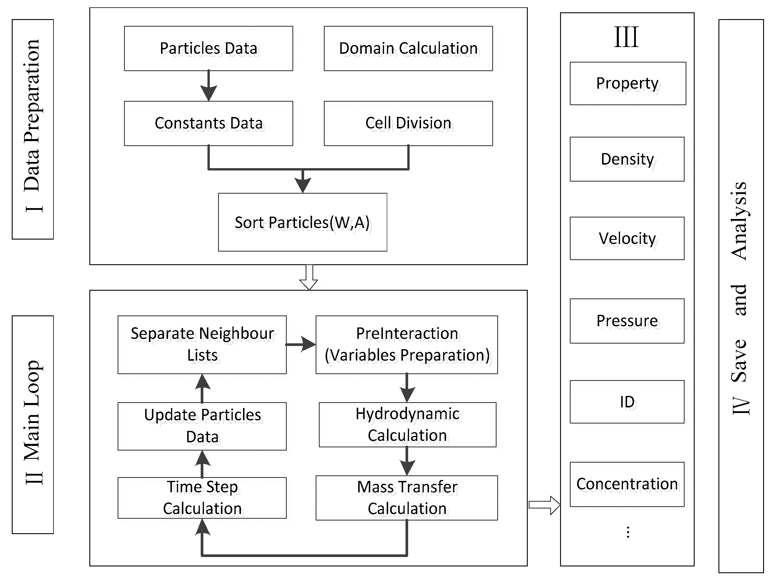
The SPH model simulation developed in this paper contains three main steps, as shown in Figure 1. (I) Data Preparation: Before the program is executed, the data must be transformed into a format that the software can identify. The data include the particle properties, the execution parameters and the calculation domain properties; (II) Main Loop: After the preparatory works are executed, the interaction of particles is executed using hydrodynamic and mass transfer calculations. This step is the core method for determining the computing time of the SPH model; and (III) Save and Analysis: The mechanical property and mass transfer process will be saved by a time series. In the analysis software, the results will be rendered and analyzed.
In each step of the SPH method, the interactions between different particles are calculated using traversal paired searches for certain particles in the computation domain, and this leads to an increased computation time. In this paper, a cell-linked list search method is used to construct the computation framework, and the computation domain is divided into “background cells” shown in Figure 2 [34]. The cell aids the numerical simulation but does not participate in it. For 2D coordinates, the cell size is the length of the support domain (2h). All of the pair-wise particle distances are less than 2h, which means all adjacent particles can only appear in the cell of the adjacent cell. For a particle that is located inside a cell, only the interactions with particles of neighboring cells must be considered. Therefore, during the force and mass transfer computation, domains without adjacent particles should not be calculated, and this greatly improves the computational efficiency.
Judgment of air-water interfaces is the premise for studying the mass transfer of dissolved gas. In the paper, the range of the mass transfer between air and water is limited to a search radius. Before computing and analyzing the mass transfer, the particle types of different phases should be defined with different symbols. In this paper, the critical function is employed within the scope of the search radius.
The meaning of function is when i and j are different phases within the search radius, the mass transfer process is computed. Otherwise, i and j are the same phases, and the mass transfer is set to 0.
In the paper, the solid boundaries are described by a set of discrete particles which are fixed in position. The momentum equations of the boundary particles are the same as water particles in the simulation. In addition, the positions of the boundary particles do not change according to the imposed forces on them, and the computer used in the simulation is an Intel® Core™ i7-4790 CPU @ 3.60 GHz; (RAM) 16.0 GB; Windows 7. By running the case for hydrodynamics simulation for 8 s, the runtime is about 9 h.
4. Validation for the Hydrodynamics over the Stepped Spillway
The hydrodynamic model was validated using the experiments carried out by Chanson et al. [5]. In this experiment, the properties of air-water flow were measured with a probe. Here, the computation domain was the same as that used in the experiment.
4.1. Description of Chanson’s Experiment
Figure 3 shows the structure of the experiment with a 21.8° slope step chute, which consisted of a broad crested weir (1 m wide, 0.6 m long) with a rounded corner (0.057 m radius) followed by nine uniform steps (hs = 0.1 m, ls = 0.25 m). The numbers from top to bottom are 1, 2, …, 9. The velocity is measured at the step edges. The change of hydraulic characteristics is monitored, when the flow rate Q is set equal to 0.058 m3/s.
The velocity monitoring points are set at steps 3–8. Here, y (m) is the longitudinal distance from the step edge surface to the monitoring point; U (m/s) is the water velocity; and (m/s) is the critical velocity. For a rectangular channel, (q is the discharge per unit width, , where w is the width of the channel). In this paper, the discharge per unit width q is 0.058 m3/s; is the critical depth, where hs (m) is the step height, ls (m) is the step length, and Hs (m) is the water elevation in the tank.
4.2. Set-Up Parameters
The parameters used for simulation of hydrodynamics are presented in Table 1.
4.3. Discussion about the Hydrodynamics Characteristics
Figure 4 shows the simulation result of the distribution of different types of particles over the stepped spillway. As shown in Figure 4, the simulation result is generally consistent with the experimental result in terms of the air water distribution and flow pattern, see Figure 3-1(B) in Chanson et al. [35]. Here, a transition flow pattern can be observed. In the third step, the air-water interface is clearly broken up and deformed. The mixed process becomes severe, and the inception point of free-surface aeration clearly appears. The numerical simulation matches the experimental. Downstream of the inception point of free-surface aeration, the kinetic energy is generated. Under this condition, water particles overcome gravity and jump away from the water surface. Thus, the mixed phenomenon can be seen clearly. Meanwhile, the nappe reattaches the water surface at the next step, and some deflected nappes fall back to the fifth and sixth step edges. In addition, when the flow passes the step edges, a certain type of fluctuation over the steps can be observed downstream of the inception point of free-surface aeration. The simulation results are in accordance with the experimental results and correctly reflect the mixing situation of the laboratory experiment.
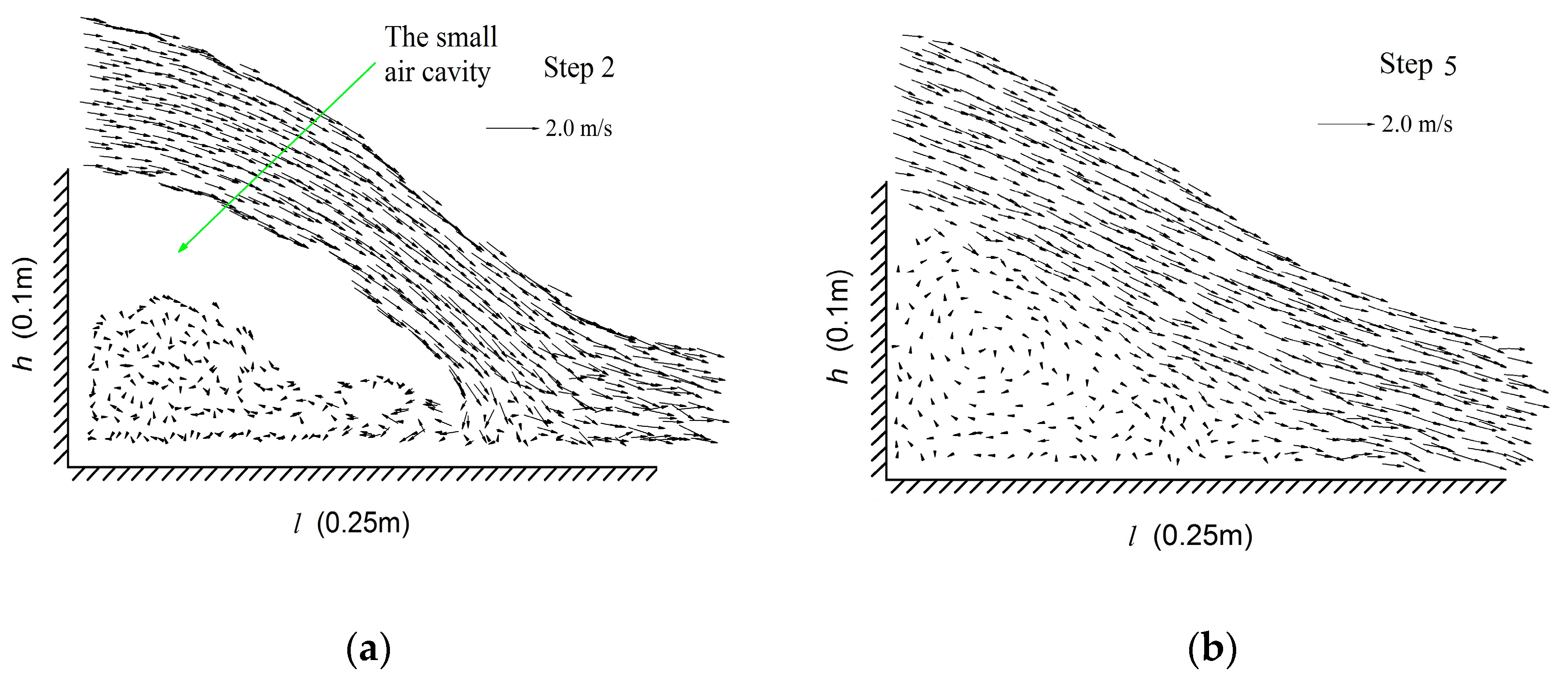
Figure 5 shows the velocity field of the water phase on Step 2 and 5. The results obtained from analyzing the velocity field of the water on the stepped spillways are more intuitive. Upstream of the inception point of free-surface aeration (Figure 5a), an obvious cavity can be observed. Downstream of the inception point of free-surface aeration (Figure 5b), the breaking degree of water increases constantly, which is typical for aeration and entrainment. Inside the steps, an expected clockwise vortex appears, and the velocity of water increases from center to the edge, which has a significant effect on energy dissipation. The main reason for velocity change inside the steps is that part of the kinetic energy of the flow will turn into heat energy, leading to velocity attenuation and energy dissipation.
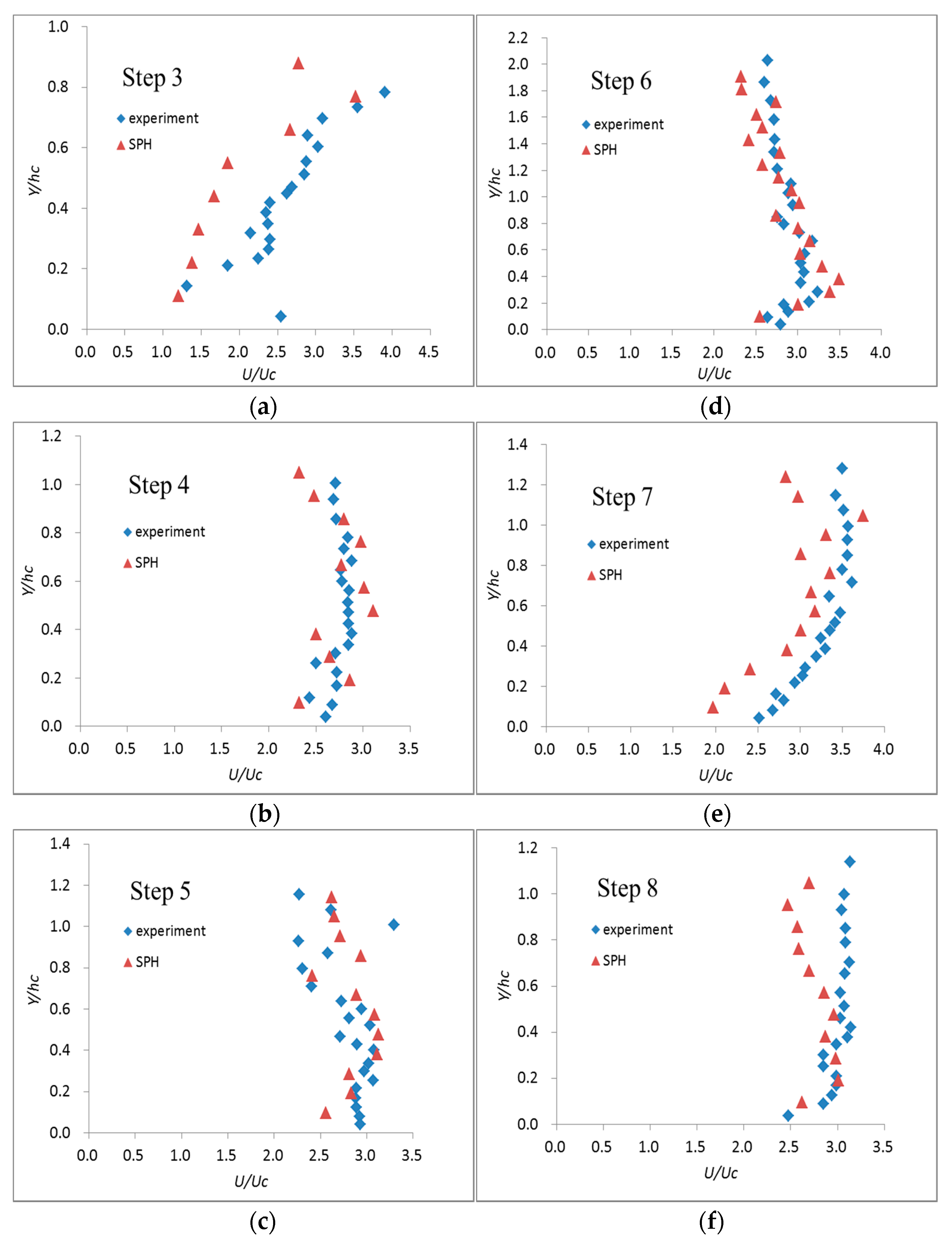
Figure 6 shows the distribution of water velocity under the condition of dimensionlessness from Step 3 to Step 8. The abscissa is U/Uc, and the ordinate is y/hc, which are Uc = 0.668 m/s and hc = 0.07 m, respectively, here. As shown in Figure 6, the numerical simulation results based on the two-phase SPH model agree well with the experimental results, except the result in Step 3, and the hydrodynamic characteristics can be correctly reflected. In Step 3, the location of the inception of free-surface aeration appears. In this step, the air-water interface edge breaks up and deforms violently, which may lead to difficulties with measurement and errors in the simulation. In general, the velocity distributions vary rapidly at different step edges. The flow velocity is larger in the interval [0.3hc, 0.8hc] than it is at other locations. When y > 0.8hc, the velocity of monitoring points fluctuates significantly. Small parts of water drop much faster than do others due to the splash effect of the previous steps. Some parts of water velocity exhibit attenuation due to the collision of the step itself, which converts kinetic energy into potential energy.
Compared to the experimental data, the two-phase SPH model presented in this paper can reflect accurately and reliably the hydrodynamic characteristics.
5. Validation for Reaeration over the Stepped Spillway
The reaeration process over the step spillway was validated using the experiment carried out by Cheng [7,8]. The computation domain was similar to the physical model with Cheng’s experiment.
5.1. Description of Cheng’s Experiment
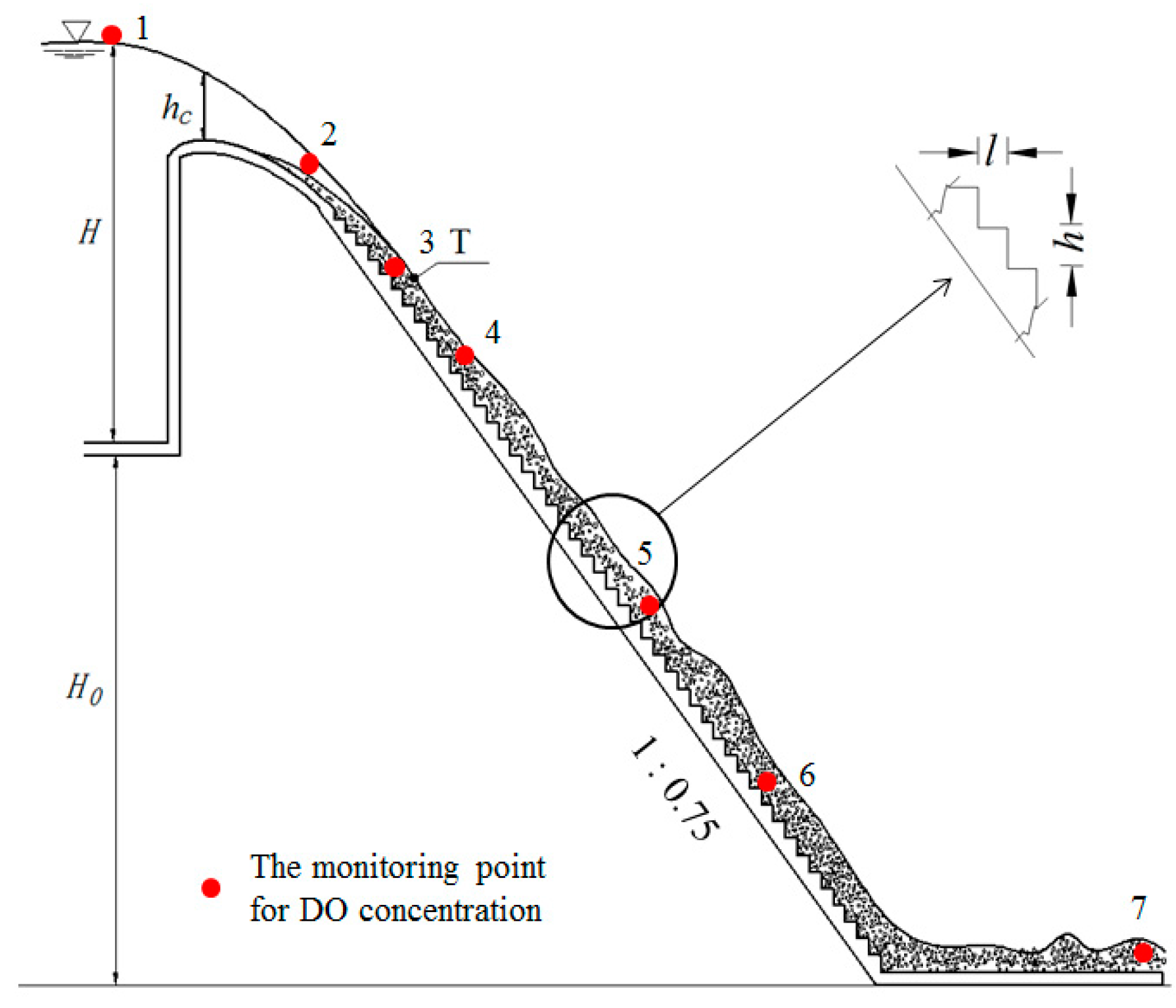
In the experiment, clear water that meets the required oxygen deficit condition is used as the experimental water. Figure 7 shows the structure of the stepped spillway. There are seven points at which the DO concentration is monitored. As shown in Figure 7, point 1 is the monitoring point for the initial DO concentration at the inlet, points 2–6 are the monitoring points on the stepped spillway surface and point 7 is the monitor point at the toe.
Table 2 shows the structural characteristics of the stepped spillway.
Where the WES curve is the surface equation of the weir crest; the weir crest meets the standard WES curve; design slope is the design grade of the spillway; T is the point of tangency of the WES curve and slope surface; steps is the number of uniform steps; hs and ls are the length and width of the step, respectively; Hs is the water elevation in the tank; q is the discharge per unit width; Cu is the concentration of DO at the weir crest; Cd is the concentration of DO at the toe; and Cs is the saturated DO concentration.
5.2. Set-up Parameters
The parameters used in the simulation are detailed in Table 3.
5.3. Discussion about the Reaeration
Figure 8 shows the results obtained for the air water distribution. The free surface line gradually decreases from crest to toe, and the line is smooth. The critical water depth hc is approximately 0.14 m, which is in agreement with the experimental data.
Figure 8 (upper right) shows the particle distributions for different phases on the stepped spillway. The mixed air and water flow formed on the step surfaces with violent turbulence and strong aeration. Some incompletely developed vortices that entrain air can also be seen inside the step.
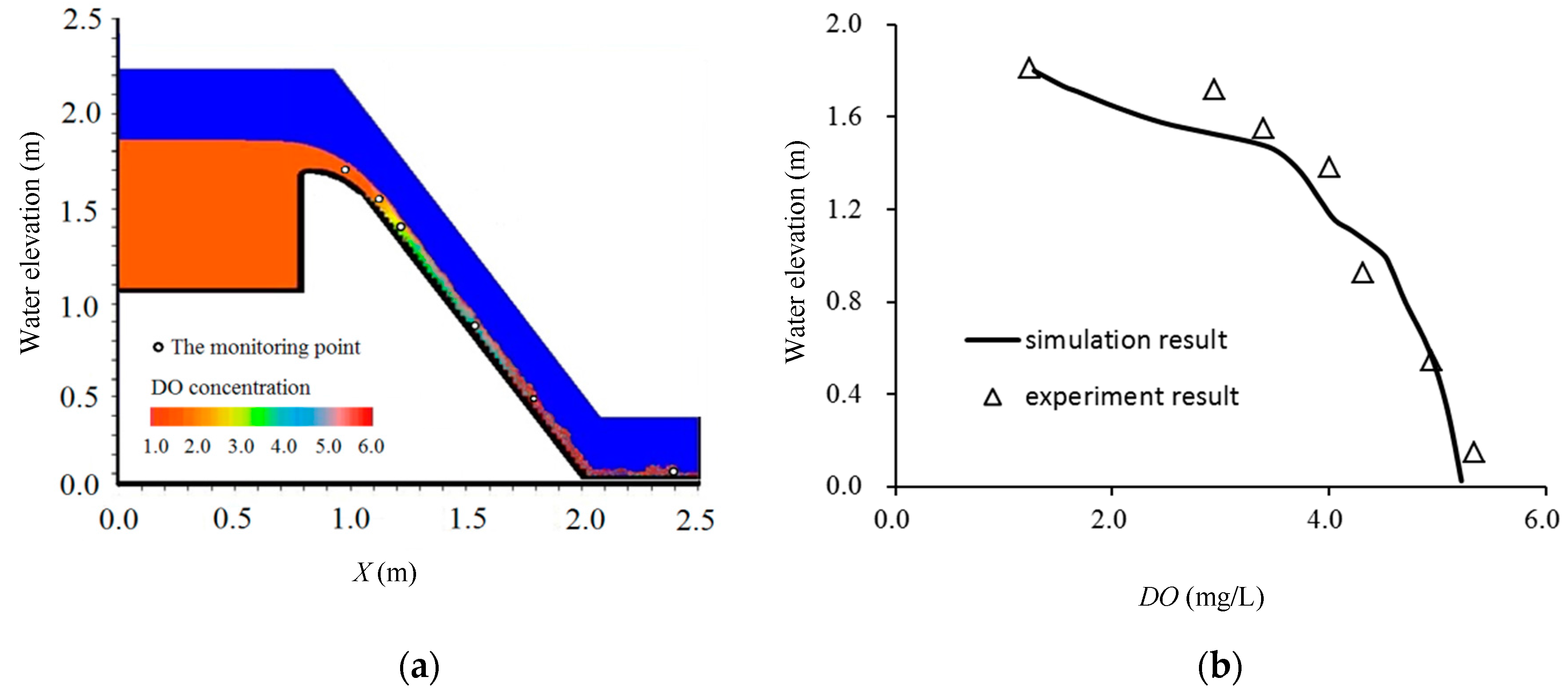
Figure 9 shows the simulation results for the progress of the DO concentration over the stepped spillway. The DO concentration gradually increases from top to toe in the horizontal direction. The DO concentration gradient decreases gradually in the normal direction along the vertical direction. The turbulence of aerated flow exhibits an accelerated diffusion of the equilibrium concentration and promotes the horizontal distribution of DO concentration.
Data comparisons at different points are given in Table 4. As shown in Table 4, the simulation results based on the two-phase SPH mass transfer model agreed with the experiment results well. The max relative error appeared at point 2 because the air entrainment at this point was not obvious. Another reason for the difference is that the measuring point is far from the water surface, which may lead to some differences between simulation and experiment results. The overall average relative error was 8.8%. Based on the analysis, we concluded that the two-phase SPH model established in the paper is capable of capturing the main features of the DO reaeration.
The reaeration rate of DO deficit, , is used to analyze the computational accuracy of the numerical simulation:
The efficiency of the reaeration rate of DO is higher when is greater. There is no DO reaeration rate when .
Table 5 shows the DO reaeration rate, , of numerical simulation and experimental results. The relative error is within 6%, which satisfies the accuracy requirement of the concentration field.
From the analysis described, the two-phase SPH mass transfer model accurately computes the reaeration of DO on the stepped spillway. The DO concentration distribution in the numerical simulation is in accordance with the experimental data. The relative error of is within 6%. The comparison results demonstrate the accuracy and reliability of the two-phase SPH mass transfer model.
6. Conclusions
To analyze the change in hydrodynamic characteristics and the dissolved oxygen concentration distribution over space and time, the advection-diffusion equation of the SPH was established in the paper. A source term was added in the two-phase SPH model. Additionally, the mass transfer coefficient calculation formula that fit the SPH method was adopted. Numerical simulations of the hydrodynamic characteristics and the mass transfer process of the stepped spillway were realized based on the two-phase mass transfer SPH model. Considering the cohesive force and source term, the two-phase mass transfer SPH model could correctly reflect the flow state, the change in velocity, the location of the inception of free-surface aeration, and the DO mass transfer process over the stepped spillway. Following Chanson’s experiment, the simulation result showed that the location of the inception of free-surface aeration appeared at the third step edge. At this step, the edge of the air-water interface broke up and deformed clearly. The recirculation vortices could be observed in the downstream of the inception of free-surface aeration. The velocity was significantly greater at the edge attachments of the steps than it was inside the vortex. Following Cheng’s experiment, the mass transfer mechanism was as follows: the DO concentration increased from crest to toe, and the vertical concentration gradient decreased gradually. This result implies that the DO diffusion accelerates from the turbulent aerated flows, which facilitates the uniform vertical distribution of the DO concentration.
Compared to the traditional mesh-based methods, the two-phase SPH mass transfer model established in this paper can simulate the large deformation and turbulent breakup flow properties, as well as the mass transfer process under strong turbulence conditions over the stepped spillway well.
Acknowledgments
This research was supported by the National Key R & D Program of China (grant No. 2016YFC0401710) and the Open Fund Project of State Key Laboratory of Hydraulics and Mountain River Engineering in Sichuan University (SKHL1305).
Author Contributions
Hang Wan and Ran Li conceived and developed the software; Carlo Gualtieri edited the manuscript; Huixia Yang contributed the section on Validation for Reaeration over the Stepped Spillway; Jingjie Feng edited the manuscript and the editorial comments; Hang Wan wrote the paper.
Conflicts of Interest
The authors declare no conflict of interest.
References
- Zhang, W.; Zhu, D.Z. Near-field mixing downstream of a multiport diffuser in a shallow river. J. Environ. Eng. 2011, 137, 230–240. [Google Scholar] [CrossRef]
- Rajaratnam, N. Skimming flow in stepped spillways. J. Hydraul. Eng. 1990, 116, 587–591. [Google Scholar] [CrossRef]
- Rice, C.E.; Kadavy, K.C. Model study of a roller compacted concrete stepped spillway. J. Hydraul. Eng. 1996, 122, 292–297. [Google Scholar] [CrossRef]
- Ruff, J.F.; Frizell, K.H. Air concentration measurements in highly-turbulent flow on a steeply-sloping chute. In Proceedings of the American Society of Civil Engineers Hydraulic Engineering Conference, Buffalo, NY, USA, 1–5 August 1994; Volume 2, pp. 999–1003. [Google Scholar]
- Chanson, H.; Toombes, L. Experimental investigations of air entrainment in transition and skimming flows down a stepped chute. Can. J. Civ. Eng. 2002, 29, 145–156. [Google Scholar] [CrossRef]
- Moog, D.B.; Jirka, G.H. Air-water gas transfer in uniform channel flow. J. Hydraul. Eng. 1999, 125, 3–10. [Google Scholar] [CrossRef]
- Cheng, X. Study on Reaeration of Sluicing Structure in River; Sichuan University: Chengdu, China, 2004. [Google Scholar]
- Cheng, X.; Luo, L.; Chen, Y.; Zhao, W. Re-Aeration Law of Water Flow over Spillways. J. Hydrodyn. Ser. B 2006, 18, 231–236. [Google Scholar]
- Chen, Q.; Dai, G.; Liu, H. Numerical simulation of overflow in stepped spillway. J. Hydraul. Eng. 2002, 33, 20–26. [Google Scholar]
- Wei, Z.; Dalrymple, R.A.; Hérault, A.; Bilotta, G.; Rustico, E.; Yeh, H. SPH modeling of dynamic impact of tsunami bore on bridge piers. Coast. Eng. 2015, 104, 26–42. [Google Scholar] [CrossRef]
- Wei, Z.; Dalrymple, R.A.; Rustico, E.; Hérault, A.; Bilotta, G. Simulation of nearshore tsunami breaking by Smoothed Particle Hydrodynamics method. J. Waterw. Port, Coast. Ocean Eng. 2016, 142, 05016001. [Google Scholar] [CrossRef]
- Federico, I.; Marrone, S.; Colagrossi, A.; Aristodemo, F.; Antuono, M. Simulating 2D open-channel flow through an SPH model. Eur. J. Mech. B/Fluids 2012, 34, 35–46. [Google Scholar] [CrossRef]
- Liu, X.; Lin, P.Z.; Shao, S.D. An ISPH simulation of coupled structure interaction with free surface flows. J. Fluids Struct. 2014, 48, 46–61. [Google Scholar] [CrossRef]
- Aristodemo, F.; Marrone, S.; Federico, I. SPH modeling of plane jets into water bodies through an inflow/outflow. Ocean Eng. 2015, 105, 160–175. [Google Scholar] [CrossRef]
- Jonsson, P.; Andreasson, P.; Hellström, J.G.I.; Jonsén, P.; Lundström, T.S. Smoothed Particle Hydrodynamic simulation of hydraulic jump using periodic open boundaries. Appl. Math. Model. 2016, 40, 8391–8405. [Google Scholar] [CrossRef]
- Colagrossi, A.; Landrini, M. Numerical simulation of interfacial flows by smoothed particle hydrodynamics. J. Comput. Phys. 2003, 191, 448–475. [Google Scholar] [CrossRef]
- Grenier, N.; Touzé, D.L.; Colagrossi, A.; Antuono, M.; Colicchio, G. Viscous bubbly flows simulation with an interface SPH model. Ocean Eng. 2013, 69, 88–102. [Google Scholar] [CrossRef]
- Das, A.K.; Das, P.K. Bubble evolution and necking at a submerged orifice for the complete range of orifice tilt. AIChE J. 2013, 59, 630–642. [Google Scholar] [CrossRef]
- Tartakovsky, A.M.; Meakin, P.; Scheibe, T.D.; West, R.M. Simulations of reactive transport and precipitation with smoothed particle hydrodynamics. J. Comput. Phys. 2007, 222, 654–672. [Google Scholar] [CrossRef]
- Aristodemo, F.; Federico, I.; Veltri, P.; Panizzo, A. Two-phase SPH modelling of advective diffusion processes. Environ. Fluid Mech. 2010, 10, 451–470. [Google Scholar] [CrossRef]
- Cleary, P.W.; Monaghan, J.J. Conduction Modelling Using Smoothed Particle Hydrodynamics. J. Comput. Phys. 1999, 148, 227–264. [Google Scholar] [CrossRef]
- Monaghan, J.J. Smoothed particle hydrodynamics. Annu. Rev. Astron. Astrophys. 1992, 30, 543–574. [Google Scholar] [CrossRef]
- Monaghan, J.J. Simulating Free Surface Flows with SPH. J. Comput. Phys. 1994, 110, 339–406. [Google Scholar] [CrossRef]
- Monaghan, J.J.; Kocharyan, A. SPH simulation of multi-phase flow. Comput. Phys. Commun. 1995, 87, 225–235. [Google Scholar] [CrossRef]
- Liu, G.R.; Liu, M.B. Smoothed Particle Hydrodynamics: A Meshfree Particle Method; World Scientific: Singapore, 2003. [Google Scholar]
- Monaghan, J.J. On the problem of penetration in particle methods. J. Comput. Phys. 1989, 82, 1–15. [Google Scholar] [CrossRef]
- Issa, R.; Lee, E.S.; Violeau, D.; Laurence, D.R. Incompressible separated flows simulations with the smoothed particle hydrodynamics gridless Method. Int. J. Numer. Methods Fluids 2005, 47, 1101–1106. [Google Scholar] [CrossRef]
- Nugent, S.; Posch, H.A. Liquid drops and surface tension with smoothed particle applied mechanics. Phys. Rev. E Stat. Phys. Plasmas Fluids Relat. Interdiscip. Top. 2000, 62 4 Pt A, 4968–4975. [Google Scholar] [CrossRef]
- Zarrati, A.R. Mathematical modeling of air-water mixtures in open channels. J. Hydraul. Res. 1994, 32, 707–720. [Google Scholar] [CrossRef]
- Banerjee, S.; MacIntyre, S. The air–water interface: Turbulence and scalar exchange. Adv. Ocean Coast. Eng. 2004, 9, 181–237. [Google Scholar]
- Price, D.J. Resolving high Reynolds numbers in smoothed particle hydrodynamics simulations of subsonic turbulence. Mon. Not. R. Astron. Soc. 2012, 420, L33–L37. [Google Scholar] [CrossRef]
- Verlet, L. Computer “Experiments” on Classical Fluids. I. Thermodynamical Properties of Lennard-Jones Molecules. Phys. Rev. 1967, 159, 98–103. [Google Scholar] [CrossRef]
- Morris, J.P.; Fox, P.J.; Zhu, Y. Modeling low Reynolds number incompressible flows using SPH. J. Comput. Phys. 1997, 136, 214–226. [Google Scholar] [CrossRef]
- Domínguez, J.M.; Crespo, A.J.C.; Gómez-Gesteira, M.; Marongiu, J.C. Neighbour lists in smoothed particle hydrodynamics. Int. J. Numer. Methods Fluids 2011, 67, 2026–2042. [Google Scholar] [CrossRef]
- Chanson, H.; Toombes, L. Experimental Investigations of Air Entrainment in Transition and Skimming Flows down a Stepped Chute: Application to Embankment Overflow Stepped Spillways; Department of Civil Engineering, University of Queensland: Queensland, Australia, 2001. [Google Scholar]
Figure 1.
Modeling steps.

Figure 2.
Background cells and air water interface.
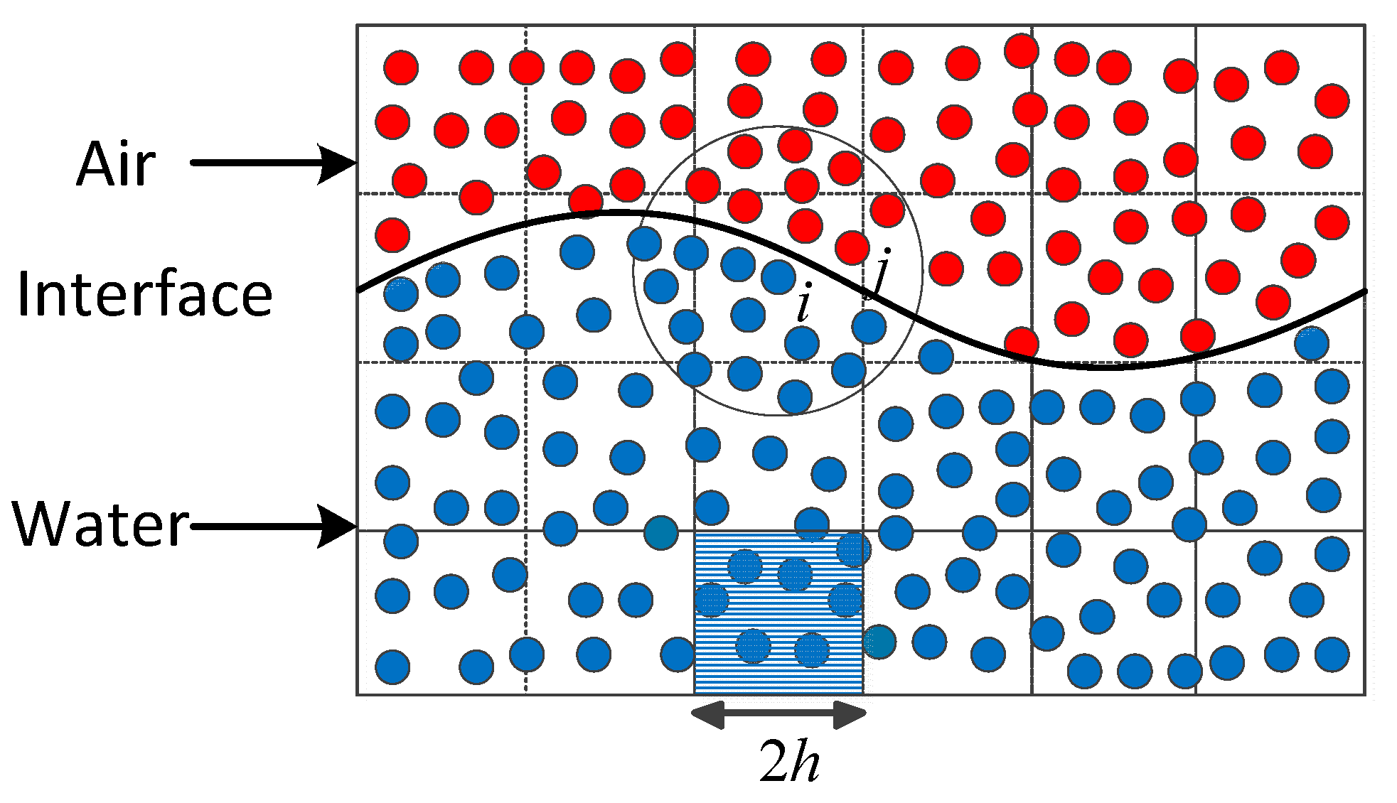
Figure 3.
Structure of the stepped spillway.
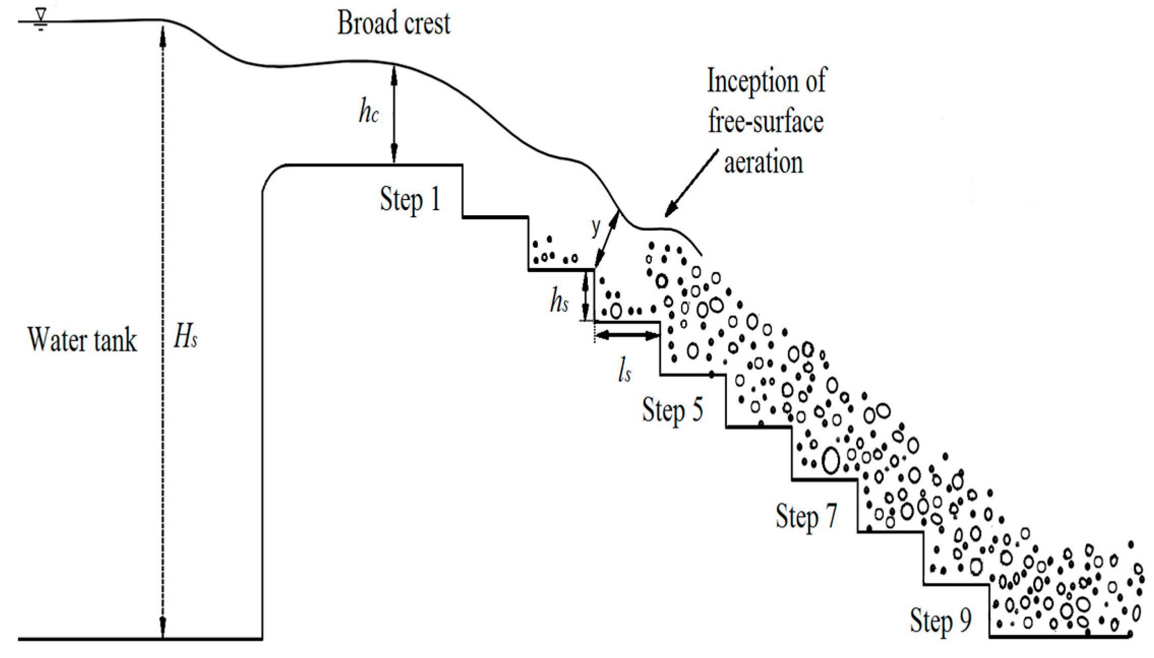
Figure 4.
Simulation results calculated using the multiphase mass transfer SPH model.
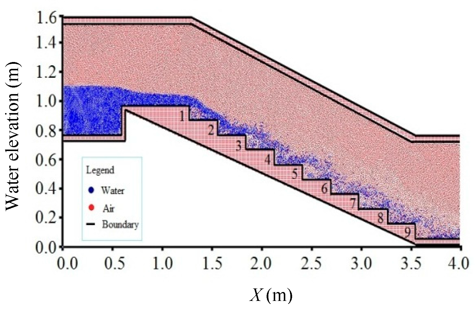
Figure 5.
The velocity field of the water phase. (a) the velocity field of the water phase on step 2, (b) the velocity field of the water phase on step 5.
Figure 5.
The velocity field of the water phase. (a) the velocity field of the water phase on step 2, (b) the velocity field of the water phase on step 5.

Figure 6.
Velocity distributions. (a) at the edge of step 3, (b) at the edge of step 4, (c) at the edge of step 5, (d) at the edge of step 6, (e) at the edge of step 7, (f) at the edge of step 8.
Figure 6.
Velocity distributions. (a) at the edge of step 3, (b) at the edge of step 4, (c) at the edge of step 5, (d) at the edge of step 6, (e) at the edge of step 7, (f) at the edge of step 8.

Figure 7.
The structure of the stepped spillway.

Figure 8.
Air water distribution over the stepped spillway.
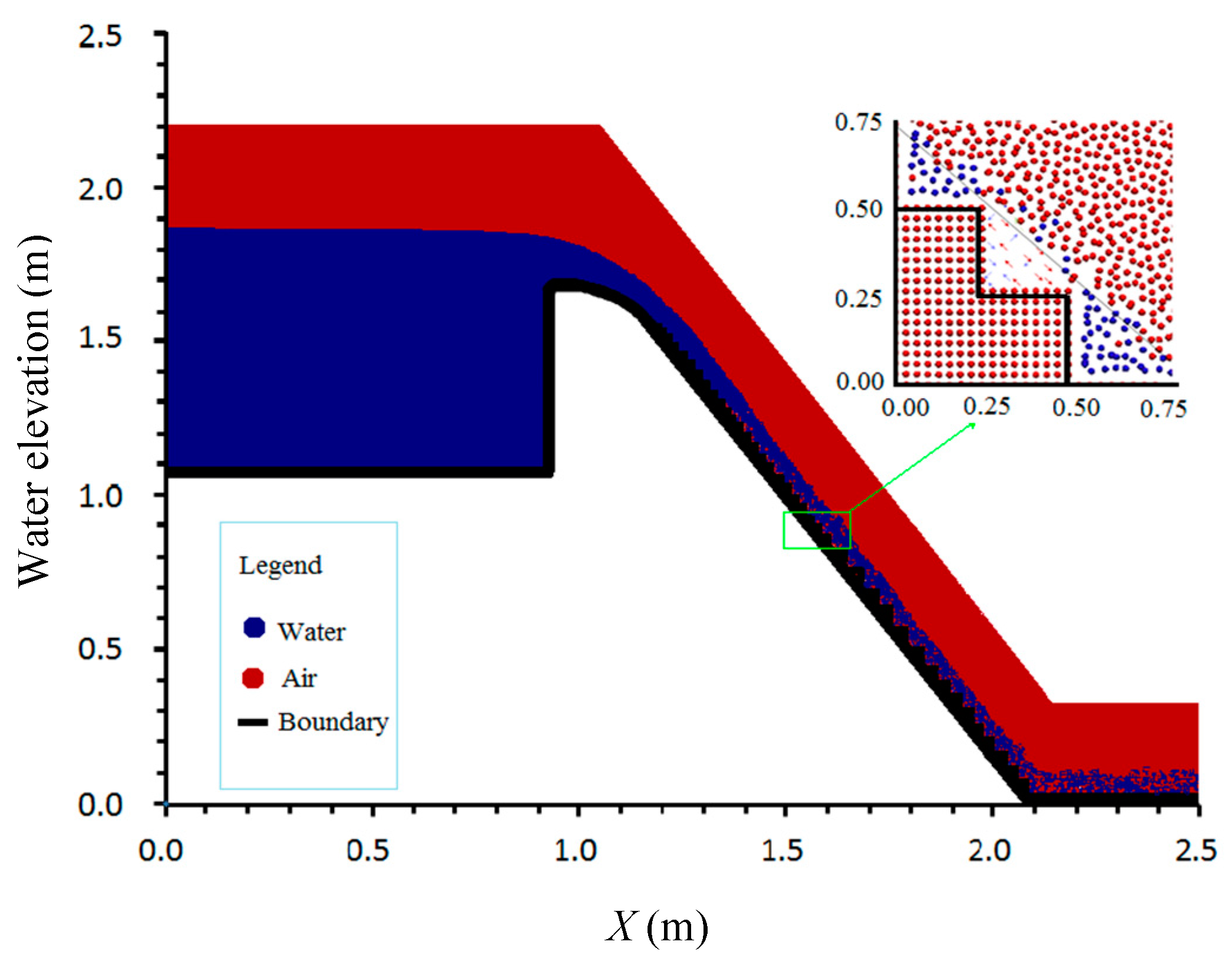
Figure 9.
(a) DO concentration distribution, (b) the comparison between experimental and simulation results.
Figure 9.
(a) DO concentration distribution, (b) the comparison between experimental and simulation results.


Table 1.
Parameters used for the simulation of hydrodynamics.
| Parameters | Water | Air | Description |
|---|---|---|---|
| (kg/m3) | 1000.00 | 1.09 | Density |
| N | 12,238 | 32,524 | Particle number |
| to (s) | 0.01 | 0.01 | Time to output |
| 7 | 1.4 | Isentropic coefficient | |
| g (m/s2) | 9.8 | 9.8 | Gravity |
| v0 (m/s) | 0 | 0 | Initial velocity |
| Kernel radius (m) | 9.8 × 10⁻³ | 9.8 × 10⁻³ | Smoothing length |
| c0 | 28.0 | 379.3 | Initial sound speed |
| Resolution (m) | 0.008 | 0.008 | Particle distance |
Table 2.
The characteristics of the stepped spillway.
| Parameters | WES Curve | Design Slope | T (m) | Steps | hs (m) × ls (m) |
|---|---|---|---|---|---|
| Values | y = 0.0304x1.85 | 1:0.75 | (0.4145, 0.2987) | 40 | 0.033 × 0.025 |
| Parameters | H0 (m) | HS (m) | q (m2/s) | Cu (mg/L) | CS (mg/L) |
| Values | 1.06 | 0.8 m | 0.0168 m2/s | 1.29 mg/L | 10.48 mg/L |
Table 3.
Parameters used for simulation of reaeration.
| Parameters | Water | Air | Description |
|---|---|---|---|
| (kg/m3) | 1000.00 | 1.09 | Density |
| N | 15,738 | 34,024 | Particle number |
| to (s) | 0.01 | 0.01 | Time to output |
| 7 | 1.4 | Isentropic coefficient | |
| g (m/s2) | 9.8 | 9.8 | Gravity |
| v0 (m/s) | 0 | 0 | Initial velocity |
| Kernel radius (m) | 4.9 × 10⁻³ | 4.9 × 10⁻³ | Smoothing length |
| c0 | 35.0 | 474.1 | Initial sound speed |
| Resolution (m) | 0.004 | 0.004 | Particle distance |
Table 4.
Comparison of the simulation and experiment results (mg/L).
| Point | 2 | 3 | 4 | 5 | 6 | 7 |
|---|---|---|---|---|---|---|
| experiment | 2.94 | 3.40 | 4.01 | 4.32 | 4.91 | 5.31 |
| simulation | 2.12 | 3.21 | 3.74 | 4.62 | 4.92 | 5.02 |
| relative error | 27.9% | 5.6% | 6.7% | −6.9% | −0.2% | 5.5% |
Table 5.
Reaeration rate of DO.
| Style | Cs (mg/L) | Cu (mg/L) | Cd (mg/L) | Relative Error | |
|---|---|---|---|---|---|
| experiment | 10.48 | 1.29 | 5.31 | 1.78 | −5.6% |
| simulation | 10.48 | 1.29 | 5.02 | 1.68 |
© 2017 by the authors. Licensee MDPI, Basel, Switzerland. This article is an open access article distributed under the terms and conditions of the Creative Commons Attribution (CC BY) license (http://creativecommons.org/licenses/by/4.0/).
Share and Cite
MDPI and ACS Style
Wan, H.; Li, R.; Gualtieri, C.; Yang, H.; Feng, J. Numerical Simulation of Hydrodynamics and Reaeration over a Stepped Spillway by the SPH Method. Water 2017, 9, 565. https://doi.org/10.3390/w9080565
AMA Style
Wan H, Li R, Gualtieri C, Yang H, Feng J. Numerical Simulation of Hydrodynamics and Reaeration over a Stepped Spillway by the SPH Method. Water. 2017; 9(8):565. https://doi.org/10.3390/w9080565
Chicago/Turabian StyleWan, Hang, Ran Li, Carlo Gualtieri, Huixia Yang, and Jingjie Feng. 2017. "Numerical Simulation of Hydrodynamics and Reaeration over a Stepped Spillway by the SPH Method" Water 9, no. 8: 565. https://doi.org/10.3390/w9080565
Note that from the first issue of 2016, this journal uses article numbers instead of page numbers. See further details here.