Analysis of Forest Fragmentation and Connectivity Using Fractal Dimension and Succolarity

Abstract

Forests around the world, vital for ecological, economic, and social functions, are facing increasing threats such as deforestation and habitat fragmentation. This study introduces “succolarity” to analyse forest connectivity and fragmentation directionally in the Romanian Carpathians from 2000 to 2021. Besides traditional indices such as the fractal fragmentation index (FFI), the fractal fragmentation and disorder index (FFDI), the local connected fractal dimension (LCFD), and succolarity, two novel indices are proposed: potential succolarity and delta (Δ) succolarity, which provide nuanced insights into environmental changes and human interventions in forests worldwide. The succolarity tests showed invariance at the image scale and sensitivity to the obstacles in different image scenarios. The combined analysis of succolarity and fractal indices reveals dynamic patterns of connectivity, fragmentation, and spatial disturbance. The directional insights of succolarity highlight and enhance understanding of deforestation patterns. The FFI and FFDI show different levels of fragmentation across mountain groups, while the LCFD details local connectivity. The adaptability of the method makes it globally applicable, supporting biodiversity conservation and landscape management. In conclusion, the integration of succolarity and traditional fractal indices provides a robust methodology for the comprehensive analysis of forest fragmentation. This advancement not only supports the sustainable management of the Romanian Carpathians but also represents a versatile approach applicable to ecosystems worldwide, ensuring the long-term resilience of forested regions.

1. Introduction

Forests are widely recognised as crucial reservoirs of ecological, economic, and social benefits [1]. However, they are currently facing a growing number of threats, particularly habitat fragmentation and loss [2,3,4]. Reports by the Food and Agriculture Organization [5] indicate that an average of approximately 10 million hectares are lost annually between 2015 and 2020. Although forests play a vital role in mitigating climate change by absorbing an impressive 2 billion tons of carbon dioxide each year [6], deforestation rates have surged to alarming levels globally. This hinders the overall effectiveness of forests in acting as carbon sinks, thereby reducing their impact on climate change [7].

For instance, deforestation and habitat fragmentation over large areas are two interrelated processes that have significant impacts on forests, forest ecosystems, and biodiversity [8,9,10,11]. The natural space for numerous species of plants and animals that rely on extensive forest areas becomes smaller and isolated with habitat fragmentation [12], which complicates the movement and migration of these species, reducing their chances of reproduction and survival [13,14,15]. The fragmentation of habitats has negative effects on the connectivity between different fragments; thus, loss of genetic diversity can impede seeding and pollination, negatively affecting natural forest regeneration [16]. Additionally, fragmentation can impact the natural resources of the forest, such as water and soil resources [17,18].

To address these complex challenges effectively, a thorough and detailed analysis of habitat fragmentation is necessary not only for developing effective conservation strategies [19,20] but also for informing ecological restoration initiatives and promoting sustainable urban development planning [21,22,23]. Various methods are available for testing [24,25,26,27,28,29,30,31] or assessing forest fragmentation, including the weighted mean patch size [32], the isolation index [33], path density [34], the shape index [35], the connectivity metrics [36,37] or the patch fragmentation index [38].

Among these methods, fractal analysis is also included. Fractal indices are a method used to measure the fragmentation and complexity of a landscape or ecosystem, including forests [39]. They have the advantage of being easy to compute and scale invariant [40]. The analysis of fractal indices can assess the impact of environmental changes and human interventions on the fragmentation and connectivity of forest habitats [41]. These indices are based on concepts from mathematics, specifically nonlinear dynamics and fractal geometry, and can provide a different perspective on how a landscape or forest is fragmented. Various measures have been proposed to quantify the degree of fragmentation in a landscape, including the box-counting dimension [42,43,44], the pyramid dimension [45,46], lacunarity [47,48,49], the Minkowski dimension [50], the Higuchi dimension [51,52], the local connected fractal dimension [53], the fractal fragmentation indices [39,54], the generalized dimension [55], or generalised entropies [56].

From a fractal perspective, existing indices such as the fractal fragmentation index (FFI) [54], the fractal fragmentation and disorder index (FFDI) [39], and the local connected fractal dimension (LCFD) [53] quantify only one characteristic of forest structure—either fragmentation, disturbance, or connectivity—globally, without considering directionality. Although these indicators provide valuable results [39,54,57,58,59,60,61,62], they do not establish a direct link between fragmentation and connectivity. Succolarity may prove useful in overcoming this limitation. It has the advantage of directionality and only quantifies dynamically connected forest patches.

However, these measures may not provide detailed information on the directionality and specific obstacles that affect connectivity between fragmented patches.

This study aims to fill the gap by using an innovative approach that leverages the concept of succolarity. This study adapts and enhances the fractal measure of succolarity to evaluate how fragmentation affects connectivity in forest areas, considering directional barriers. Succolarity was originally designed to measure the permeability of fragmented images, specifically the degree to which “virtual water” can permeate a binary image [63,64,65]. In this context, white pixels represent obstacles, while black pixels represent pathways or connectivity for said virtual water. To analyse forests using succolarity, a fractal concept for quantifying percolation, i.e., tree cover, is defined as those areas where virtual water can percolate, similar to a lake (represented by black pixels). Areas without forests are considered obstacles that force the virtual water to bypass or be blocked (represented by white pixels), such as the space between some lakes. This study presents a novel method for evaluating the impact of fragmentation on connectivity in forested regions, taking into account directional barriers.

The results of our succolarity analysis [65] are compared with three existing fractal models: the fractal fragmentation index [54], the fractal fragmentation and disorder index [39], and the local connected fractal dimension [53].

In Section 2.1, Section 2.2, Section 2.3, Section 2.4, Section 2.5, Section 2.6 and Section 2.7, the different scenarios introduced for the fractal indices are described and provided essential support for ensuring the efficacy of the two new concepts proposed in this study—potential succolarity and Δ succolarity—in better understanding percolation expansion and forest landscape dynamics for the tree cover database employed. The advantages and limitations are discussed in Section 4 in some detail.

This research analyses images of forest areas in the central regions of 10 mountain groups in the Romanian Carpathians between 2000 and 2021 that are undergoing an intensive process of deforestation, both legal and illegal, for economic purposes such as timber production for export, the expansion of residential areas, or the establishment of new tourist facilities [57,61,62,66]. The choice of this case study is driven by the significant reduction in bear habitats in the Carpathians, forcing bears to enter human settlements in search of food. Thus, quantifying the degree of fragmentation and connectivity, correlated with potential connectivity, could identify potential areas for habitat restoration [67] that would significantly reduce bear–human interactions, especially considering the protected status of bears [68,69,70,71,72,73].

This research presents a noteworthy methodological improvement in quantifying the effects of deforestation and forest loss in the Romanian Carpathians. A better comprehension of the dynamics of forested regions provides significant opportunities for preserving biodiversity and ensuring the long-term sustainability of these mountain ecosystems.

The use of succolarity can offer valuable insights into the effects of fragmentation on connectivity. This can aid stakeholders in making informed decisions for sustainable forest planning and management as well as assist them in ecological reconstruction efforts. This approach aims to reconnect forested areas to ensure optimal the continuity of habitats for endangered species.

2. Materials and Methods

This study examines the impact of deforestation on the compactness and connectivity of tree cover in the Carpathian Mountains. This analysis was conducted using succolarity, fractal fragmentation indices, and the local connected fractal dimension to analyse sets of generated and edited images within a case study framework. The images used were obtained from the Global Land Analysis and Discovery database [74] (https://glad.earthengine.app/view/global-forest-change; accessed on 19 April 2022). The following sections will describe each analytical method and type of image used. The goal is to provide a comprehensive understanding of the research approach.

2.1. Succolarity

This study investigates the use of succolarity, a metric which measures the degree of percolation of an image under analysis.

Succolarity (σ), along with fractal dimension (FD) and lacunarity (λ), are fractal measures evaluators. Fractal dimension indicates how much an object occupies its underlying metric space, while lacunarity examines the distribution of gaps or lacuna [75]. In contrast, succolarity quantifies the ability of “virtual water” to flow in an image. Succolarity is defined as an assessment of the degree to which filaments facilitate percolation or flow through an image [63].

To analyse forest patch fragmentation and connectivity from an ecological perspective, we have adopted a specific convention for our succolarity analysis. We interpret forest patches extracted from satellite images as interconnected or isolated lakes/seas, while non-forested or deforested surfaces are considered analogous to dry land between the lakes/seas.

The forest patches allow virtual water to infiltrate and flow, while the non-forested surfaces, including the deforested areas, act as obstacles around which virtual water must detour or come to a halt. Figure 1a,b depict the interconnection scenario among three hypothetical forest patches (similar to three lakes/seas). Virtual water can flow from one patch to another depending on the analysed flow direction. In this example, the analysis direction is from top to bottom (Figure 1b—green arrow). Figure 1c shows that, if the three forest patches are interconnected, virtual water from patch 1 reaches both patch 2 and patch 3 through connecting pathways, similar to water from the first lake feeding the second and then the third lake (with red is depicted percolation and with blue non-percolation after the obstacle).

If the interconnection between patches, similar to channels through which lakes communicate with each other, is disrupted (as shown in Figure 1d), only two out of the initially interconnected three patches remain connected but without percolation. This is because an obstacle has emerged, preventing the flow of virtual water. As a result, virtual water only flows within the first patch, leaving the second and third patches isolated. This prevents animals from moving between patches 2 and 3 to patch 1. If the connection between patch 2 and patch 3 is disrupted due to deforestation, patch 1 and 2 will still be connected, allowing for virtual percolation, while patch 3 will be isolated (refer to Figure 1e).

If deforestation eliminates both connections, all three patches become isolated, and percolation only occurs in the first patch when analysed from top to bottom (see Figure 1f). However, if new forest corridors are created through reforestation (see Figure 1g, magenta colour), the three patches become interconnected, restoring mobility between them (Figure 1h) (similar to the construction of channels which interconnect three isolated lakes).

Succolarity quantifies the degree of percolation in an image, representing the volume of liquid that can pass through. It measures how much of a given liquid can penetrate an image through black pixels, considering white pixels as obstacles when analysing 2D images.

The succolarity algorithm assesses the ability of virtual water to percolate in a given direction, providing insight into the spatial compaction and connectivity characteristics of objects (such as tree cover). Each pixel is categorised as either empty (black pixels, symbolizing fluid access paths in the case study, i.e., tree cover) or filled with an impenetrable mass (white pixels, symbolizing obstacles in the case study, i.e., areas without forest, including deforestation effects) to assess this percolation capability.

De Melo and Conci (2013) describe the principles of calculating percolation ability using a box-counting approach for 2D images [65]. Thus, the virtual water pressure values applied to the images depend on the number of pixels and the scale of box-counting in each direction.

Fluid flow is simulated through all the connected tree cover pixels (black pixels) in each direction, while fluid is restricted from flowing through the obstacle pixels (white pixels). The area of fluid flow being targeted is divided into equal-sized boxes in the images, which are referred to as “BS(k)”. Here, “k” represents the number of possible box-counting partitions in an image. The occupancy percentage for each image box size is directly measured on the images and noted as “OP(BS(k))”. The pressure value for each box size k is calculated using Equation (1).

$${{\displaystyle \sum }}_{k=1}^{n}OP\left(\mathrm{BS}\left(k\right)\right)\mathrm{xPR}\left(\mathrm{BS}\left(k\right),\mathrm{pc}\right)$$

(1)

where “n” represents the number of possible divisions, and “PR(BS(k),pc” represents the pressure at the centroid of box “k” in the scale of consideration.

To ensure that the succolarity value is dimensionless, this value is obtained by dividing the pressure occupancy value by the maximum possible pressure occupancy value (Equation (2)).

$$\sigma \left(\mathrm{BS}\left(k\right),\mathrm{dir}\right)=\frac{{{\displaystyle \sum }}_{k=1}^{n}OP\left(\mathrm{BS}\left(k\right)\right)\mathrm{xPR}\left(\mathrm{BS}\left(k\right),\mathrm{pc}\right)}{{{\displaystyle \sum }}_{k=1}^{n}OP\left(\mathrm{BS}\left(k\right)\right)\mathrm{xmaxPR}\left(\mathrm{BS}\left(k\right),\mathrm{pc}\right)}$$

(2)

The variable “dir” represents the direction, such as left-to-right (l2r) or right-to-left (r2l) and top-to-down (t2d) or down-to-top (d2t). The variable “max” represents the maximum pressure assignment.

The succolarity value, which ranges from 0 to 1, reflects the permeability of the image. If an image contains both white obstacle pixels and black percolation pixels, the succolarity values will fall between 0 and 1. A succolarity of 0 occurs when the entire image is white (waterproof image) or when the border (edge) in the flow direction is completely white, preventing water penetration. A value of 1 indicates unrestricted fluid flow, where the inner image is black. In this case study, succolarity is observed to increase with a higher permeability, which is characterized by larger interconnected black patches (tree cover) amid the white background (not forested or deforested areas). On the other hand, a lower permeability, which leads to fewer or smaller black connected patches, results in lower succolarity values.

To capture variations in the percolation direction, there can be calculated five succolarity values based on the direction of the virtual water flow: top-to-down (t2d), down-to-top (d2t), left-to-right (l2r), right-to-left (r2l), and the mean succolarity for all four directions. The mean succolarity provides a comprehensive overview of the percolation characteristics across different flow directions.

2.2. Potential Succolarity

Potential succolarity is a new concept that is proposed in this paper to indicate the extent to which the degree of percolation could be extended if obstacles isolating part of the patches could be penetrated.

The potential succolarity is calculated using Equation (3):

$$Potential succolarity=\frac{black pixels}{total pixels}$$

(3)

Potential succolarity does not distinguish between the four directions but rather provides a global overview.

2.3. Delta (Δ) Succolarity

Δ succolarity is also proposed as a new concept, representing the difference between potential succolarity and succolarity (Equation (4)):

$$\Delta succolarity=Potential succolarity-succolarity$$

(4)

Δ succolarity provides information on how much percolation could be further extended, considering the four flow directions, if obstacles isolating part of the patches could be penetrated.

Succolarity, potential succolarity, and Δ succolarity were calculated using the succolarity plugin from the ComsystanJ (Complex Systems Analysis for ImageJ) [76] collection plugins version 1.1.2 of Fiji/ImageJ2 2.14.0/1.54h java 1.8.0_322 64-bit [77]. Succolarity is a binary algorithm that operates on a [0, >0] scale by flooding the black pixels of a binary image. Therefore, the input images must be in an 8-bit binary format. The number of boxes for the regression parameters was set to 7, 8, 9, 10, and 11 for image scales of 64 × 64, 128 × 128, 256 × 256, 512 × 512, and 1024 × 1024, respectively. For the Romanian Carpathian forest area images, which had an image scale of 1000 × 1000 pixels, the number of boxes for the regression parameters was set to 10. The scanning type selected was the raster box.

2.4. Fractal Fragmentation Index (FFI)

The fractal fragmentation index (FFI) is a fractal index that uses multiscale fractal techniques to measure the degree of fragmentation or compression exhibited by objects occupying a space [54]. The FFI can also assess the deviation of the shape of each object from a geometric Euclidean shape. The calculation of the FFI is determined using the following Equation (5):

$$FFI=D_A-D_P=\underset{\epsilon \to 0}{ \lim }\left(\frac{\log N\left(\epsilon \right)}{\log \frac{1}{\epsilon }}\right)-\underset{\epsilon \to 0}{\lim }\left(\frac{\log N^{\prime }\left(\epsilon \right)}{\log \frac{1}{\epsilon }}\right)$$

(5)

where FFI is the fractal fragmentation index; D_A is the fractal size of the summed areas, representing the size of the box required to cover the object area; D_P is the fractal size of the accumulated perimeters, representing the size of the box required to cover only the object perimeter; ε represents the size of the box used in the analysis; logN(ε) represents the number of contiguous and non-overlapping boxes required to cover the object area; and logN’(ε) represents the number of contiguous and non-overlapping boxes required to cover only the object perimeter.

There are three situations, as follows:

• FFI = 0: This situation occurs when forest areas are very small, typically 1–4 pixels for an object. In such cases, the perimeter image using the outline function appears to be similar to the area image, with D_A = D_P. In practice, when analysing very small fractal objects or entities, it is important to recognise the limitations associated with the accurate extraction of their contours. The accuracy of contour extraction can be compromised when dealing with diminutive fractal entities, potentially affecting the reliability and interpretability of the fractal fragmentation index (FFI) calculations for these specific entities. Careful consideration of these limitations is essential to ensure the meaningful interpretation of FFI results, particularly in cases involving small fractal structures.
• 0 < FFI < 1: In scenarios where the areas occupied by objects are large and compact, the FFI value is high and close to 1, indicating that the objects are densely packed. Conversely, if the objects are more scattered, smaller, or fewer in number, or if they have a tentacular, irregular, and sprawling pattern, the FFI value decreases and approaches 0.
• FFI = 1: This situation is recorded when the area is geometrically perfect and 100% compact, without any discontinuity (D_A = 2 and D_P = 1) [54].

2.5. Fractal Fragmentation and Disorder Index (FFDI)

The fractal fragmentation and disorder index (FFDI) uses multiscale fractal techniques to quantify the degree of fragmentation, compaction, and spatial disorder exhibited by the objects filling a space [39]. This index is an extension of the FFI and incorporates aspects of the information dimension (D₁) [78]. Similar to the FFI, the FFDI distinguishes patterns of spatial organisation in processed images.

The calculation of the FFDI is determined using the following Equation (6):

$$\mathrm{FFDI}=D_1\left(1-\mathrm{FFI}\right)=\left(\underset{\epsilon \to 0}{\lim }{{\displaystyle \sum }}_{i=1}^{N\left(\epsilon \right)}\frac{m_i\left(\epsilon \right)\log \left(m_i\left(\epsilon \right)\right)}{\log \left(\epsilon \right)}\right)\left(1-\left(\underset{\epsilon \to 0}{\lim }\left(\frac{\log N\left(\epsilon \right)}{\log \frac{1}{\epsilon }}\right)-\underset{\epsilon \to 0}{\lim }\left(\frac{\log N^{\prime }\left(\epsilon \right)}{\log \frac{1}{\epsilon }}\right)\right)\right)$$

(6)

where mi = Mi/M, M_i is the number of points in the ith box; M is the total number of points of the objects; ε represents the size of the box used in the analysis; logN(ε) represents the number of contiguous and non-overlapping boxes required to cover the object area; and logN’(ε) represents the number of contiguous and non-overlapping boxes required to cover only the object perimeter.

In this Equation (6), 1 − FFI is used because FFI = 0 indicates fragmentation, and FFI = 1 indicates a lack of fragmentation. The FFDI ranges from 0 to 2. The maximum value of the FFDI approaches 2 when the objects are highly disordered and fragmented, indicating a highly disordered spatial arrangement. Conversely, the lowest value approaches 0 when the objects are weakly disordered and compact, indicating a more ordered and compact spatial organisation.

The FFI and FFDI were calculated using the fractal fragmentation indices plugin available in the ComsystanJ collection plugins [76] for Fiji/ImageJ2 2.14.0/1.54h [77]. These plugins provide binary algorithms that operate on a [0, >0] scale by analysing the white pixels of a binary image. Therefore, it is imperative that the input images are in an 8-bit binary format, inversely configured compared to the images used for the succolarity analysis.

To be consistent with the succolarity analysis, the number of boxes for the regression parameters was set to 7, 8, 9, 10, and 11 for image scales of 64 × 64, 128 × 128, 256 × 256, 512 × 512, and 1024 × 1024, respectively. For the Romanian Carpathian forest area images, which had an image scale of 1000 × 1000 pixels, the number of boxes for the regression parameters was set to 10.

Note that succolarity-compatible images require inversion using Fiji/ImageJ2 2.14.0/1.54h (Edit–Invert). This inversion ensures that white pixels correspond to the tree cover, while black pixels represent the background areas without forest, including deforestation effects.

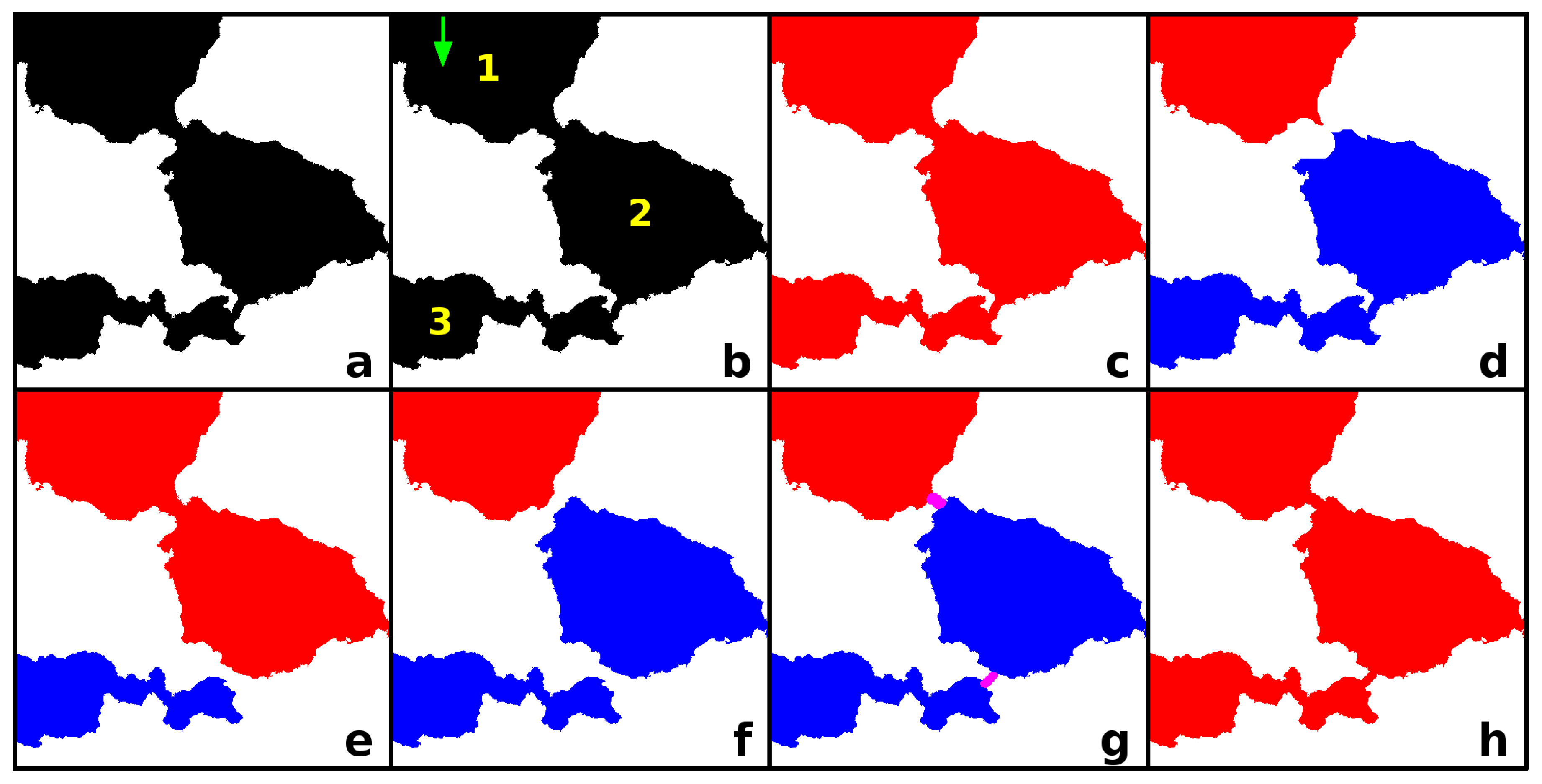
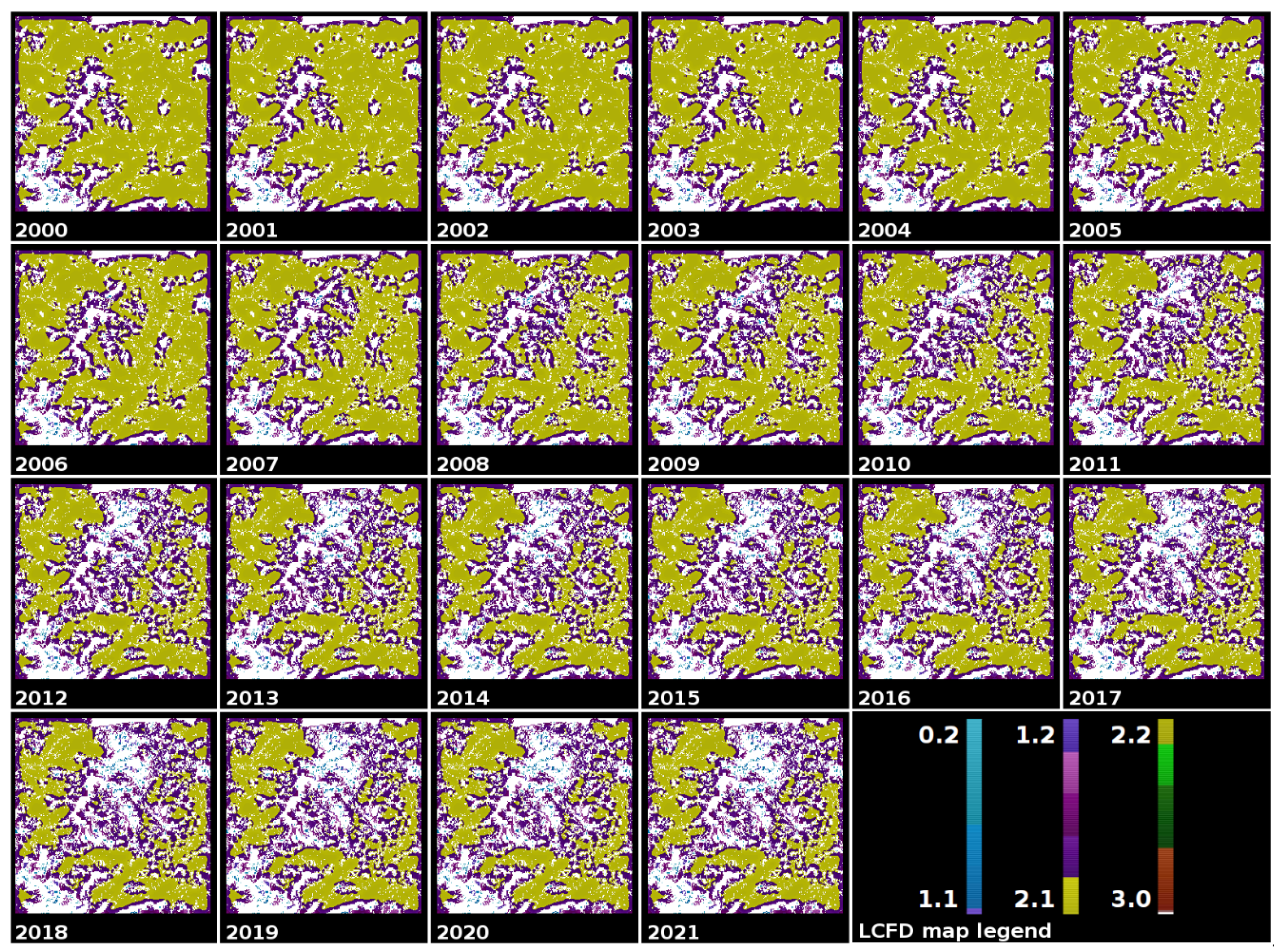
2.6. Local Connected Fractal Dimension (LCFD)

The local connected fractal dimension (LCFD) is a fractal index used to quantify local connectivity. It is expressed according to Equations (7) and (8):

$$M\left(ϵ\right)\propto F{ϵ}^{LCFD}$$

(7)

$$LCFD=\frac{log\left[M\left(ϵ\right)\right]}{log\left(ϵ\right)}$$

(8)

where F is a mass prefactor, and M(ε) is the number of locally connected pixels (an eight-neighbour connection) in a box ε [53,79].

The LCFD value is 1 if the object is a straight one-dimensional line and 2 if the object is two-dimensional and completely covered. The determination of connectivity is based on considering pixels within the 8 × 8 environment of the starter pixel as connected, following the basic rule for identifying connected sets within a given arbitrary distance around the base pixel.

LCFD estimation was performed using the FracLac plugin [80] for the Fiji/ImageJ2 2.14.0/1.54h [77]. In this analysis, binary images were imported into FracLac as a binary stack. The local connected fractal dimension option was selected with black as the background for the fractal connectivity analysis. The result included an average of all connectivity values per image.

2.7. Image Generation for Testing and Validating Succolarity

The aim of generating images was to evaluate and validate succolarity’s ability to quantify the degree of fragmentation, compaction, and interconnection. This evaluation aimed to assess succolarity’s performance in relation to directionality.

Firstly, five sets, each containing six images, were generated using the Fiji/ImageJ2 2.14.0/1.54h software [77]. The sets consisted of three isotropic images (black square, cross, and white square) as well as three anisotropic images (three-quarter square, half square, and quarter square). The images were generated at scales of 64 × 64, 128 × 128, 256 × 256, 512 × 512, and 1024 × 1024 pixels (Figure 2). This process aimed to assess the sensitivity of succolarity to variations in image scale, mirroring the approach taken in our fractal analysis. To prevent potential biases introduced by automatic resizing and other error sources, it was essential to ensure uniformity in scale (pixel size) and extent when comparing images for the fractal analysis. As highlighted by Loke and Chisholm (2022), this standardization applies to both algorithmically generated images and those derived from empirical data [81].

Secondly, the Image generator—Fractal HRM from ComsystanJ collection plugin [76] was used within the Fiji/ImageJ2 2.14.0/1.54h software to generate a hierarchically structured random map (HRM) image. The HRM image was created using a recursive algorithm inspired by the curdling and random trema generation method introduced by Plotnick [27,63]. HRMs are maps of pixels randomly assigned values of 0 or 1, with varying probability distributions in different regions. These maps can simulate landscapes with varying levels of clustering, fragmentation, and connectivity, achieved through the processes of curdling and random trema. It is important to note that two surfaces may share the same overall fill space and yet diverge in their degree of curdling, which denotes the clustering or nucleation of the filled space. The unfilled space is created through a random process called trema, which involves placing holes with a defined shape on the mathematical surface [25,26,63].

The HRM image for this experiment was generated at a scale of 512 × 512 pixels, corresponding to 262,144 pixels, with a fixed number of 512 rows and columns (M) (Figure 3a). The image falls under category s1, which is denoted as “high” (refer to [39] for comprehensive details). Specific probability values were assigned: p1 = 0.5 and p2 = p3 = 1. The variables p1, p2, and p3 represent the percentage of space occupied by HRM objects at different grain sizes, expressed as a fraction (e.g., 0.5 corresponds to 50%). Specifically, p1 corresponds to a grain size of 50 × 50 pixels, p2 to 5 × 5 pixels, and p3 corresponds to 1 × 1 pixel. These variations in grain size enable the examination of HRM objects at different scales within the fixed scale of the 512 × 512-pixel HRM image. The image produced is anisotropic, making it appropriate for a succolarity analysis in all four directions: t2d, d2t, l2r, and r2l (Figure 3b–e).

Thirdly, the HRM image was edited to enable more detailed tests of succolarity.

-

The first edit included adding a horizontal white line, four pixels thick, in the initial optimum of the image (Figure 3g; for better visualisation, the line is shown in yellow in the figure). When a barrier is completely impenetrable, fluid flow stops, and the black pixels beyond the barrier are not measured. This is because the barrier acts as an impermeable layer, blocking the virtual liquid above. A new concept, Δ succolarity, was introduced to quantify these black pixels located beyond the barrier. Together with the quantifiable pixels located in front of the barrier, they formed the potential succolarity, another proposed concept. The aim of this approach was to measure the effect of a continuous obstacle on the flow of virtual water. The evaluation focused on the four directions of analysis (t2d, d2t, l2r, and r2l) (Figure 3h–k), with a particular emphasis on t2d and d2t (Figure 3h,i). Figure 3h–k depict the four percolations limited by the presence of the barrier, corresponding to the four analysed directions. To aid visualization, the black pixels located beyond the barrier and thus not quantified are represented in grey.

-

In the second edit, the HRM image was framed by a white border that was 12 pixels wide (Figure 3f). The purpose of this edit was to measure succolarity when the image was completely impermeable to water (Figure 3l). In the presence of a white border, which acts as a continuous external obstacle in all four directions, all black pixels that could potentially allow percolation are considered “inactive”. This is because the border prevents virtual liquid from penetrating the image. In this scenario, these “inactive” black pixels represent both the potential and Δ succolarity, as their succolarity is equal to 0. These “inactive” black pixels are located beyond the image border (see Figure 3f) and are displayed in grey for clarity (see Figure 3l).

-

In the third edit, two black pixels that connected two patches in the original image were removed (as shown by the red line in Figure 3m and by the white in Figure 3n). Figure 3o–r show the four percolations corresponding to the four analysed directions. Two black pixels were removed, creating a small white barrier between the two patches. It is evident that breaking a connection between two patches deactivates some black pixels beyond the rupture of that connection. These pixels no longer facilitate “flow” and become “inactive” due to the obstacle created. To improve visualization, grey pixels located beyond the connection rupture and, therefore, not quantified represent these black pixels. The aim was to identify changes in succolarity when interconnections became obstacles (Figure 3o–r).

These second and third edits provided essential support for validating the two new concepts proposed in this study: potential succolarity and Δ succolarity.

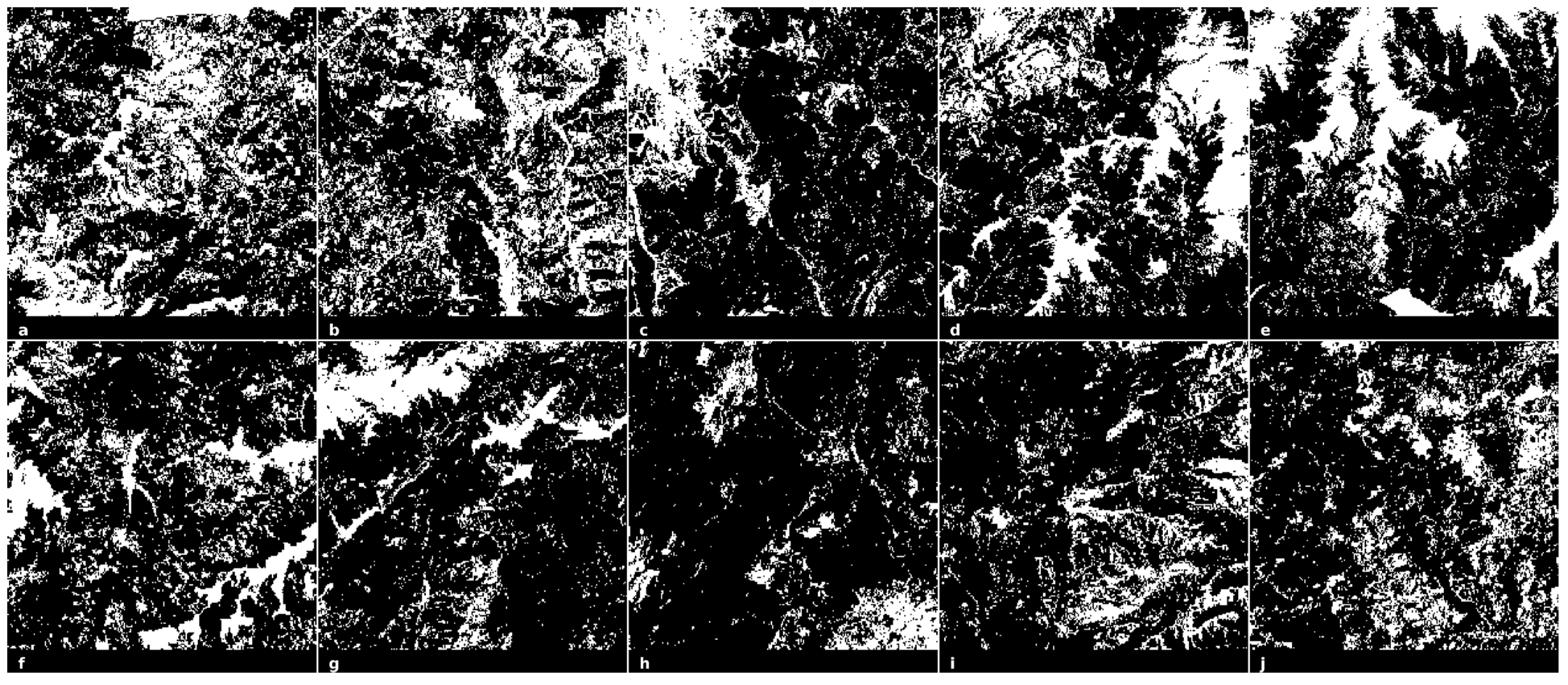
2.8. Tree Cover Images of the Romanian Carpathians Mountains

In the current research, the tree cover database for 2001–2021 from a previous research study (available as supplementary material [39] was used (https://static-content.springer.com/esm/art%3A10.1007%2Fs10980-023-01640-y/MediaObjects/10980_2023_1640_MOESM4_ESM.zip; accesed on 19 September 2023). The images were processed from the Global Land Analysis and Discovery database [74] (https://glad.earthengine.app/view/global-forest-change; accessed on 19 April 2022). The methodology for obtaining these images and preprocessing them to generate the final images is described in [39]. The study area is a significant geographical region with mountainous terrain forming a circular arc that stretches from the northern border with Ukraine to the southern border with Serbia (Figure 4).

Ten stacks of twenty-two images each were analysed, one image for each year of the analysed time interval, from 2000 to 2021. The ten stacks corresponded to the ten mountain groups of the Romanian Carpathians: the Northern Eastern Carpathians, Central Eastern Carpathians, Southern Eastern Carpathians, Bucegi, Făgăraș, Parâng, Retezat–Godeanu, Banat, Poiana Ruscă, and Apuseni mountain groups (Figure 5). The size of all the images was 1000 × 1000 pixels. Black pixels corresponded to forest cover and white pixels to non-forest or deforested areas for the succolarity analysis and the opposite for the FFI, FFDI, and LCFD analyses.

3. Results

This section presents the results of the succolarity analysis, focusing on the impact of the black patches’ sizes and their connectivity on the obtained values. Succolarity values, which range from 0 to 1, serve as a significant indicator for assessing image permeability. The importance of the interaction between white and black pixels is highlighted by the distinction between low and high succolarity. The variability in succolarity is revealed by exploring the dimensions and connections of black patches, providing a detailed perspective on how these features impact image permeability.

The study used test images from Figure 1 and Figure 2 to explore the capability of succolarity in quantifying the degree of fragmentation/compactness and connectivity of areas with black pixels that facilitate percolation against a background composed of white obstacle pixels. Additionally, the test images were analysed for comparison with three fractal indices: FFI, FFDI, and LCFD. After validation, succolarity was used to investigate the impact of deforestation on the density and connectivity of forest fragments over a 22-year period in ten mountainous regions of the Romanian Carpathians.

3.1. Invariance of Succolarity to Image Scale

This section explores the consistent behaviour of succolarity with respect to image scale. The analysis reveals that succolarity remains invariant across varying image scales, consistently presenting identical values irrespective of an image’s dimensions, whether these are 64 × 64, 128 × 128, 256 × 256, 512 × 512, or 1024 × 1024 pixels (refer to Figure 6a).

However, the three analysed fractal dimensions (FFI (Figure 6b), FFDI (Figure 6c), and LCDF (Figure 6d)) are sensitive to image size. The FFI values increase proportionally with image scale (ranging from 64 × 64 pixels to 1024 × 1024 pixels), which introduces a bias in the analysis. For example, the FFI for a half-square image with dimensions of 1024 × 1024 pixels is higher than the FFI for a quarter-square image with dimensions of 256 × 256 pixels. As a result, larger images, such as those with dimensions of 1024 × 1024 pixels, exhibit higher compactness values compared to smaller images, such as those with dimensions of 512 × 512 pixels, even if they have identical texture and structure. This difference is due to the larger number of pixels being analysed.

The FFDI values decrease as image dimensions increase, resulting in larger images (1024 × 1024) showing higher compactness and order values while maintaining uniform texture and structure. The LCDF values show a slight increase, from smaller image dimensions (64 × 64) to larger ones (1024 × 1024), indicating a slightly higher degree of connectivity while maintaining consistent texture and structure.

In the case of black images, which consist solely of foreground pixels, they achieve an FFI value of 1 and an FFDI value of 0, regardless of the image’s size. Conversely, white images consisting solely of background pixels yield an FFI score of 0 due to the absence of quantifiable pixels. As a result, there is no connectivity (LCDF = 0), making it impossible to calculate the informational dimension, resulting in the FFDI consistently being NaN.

It is important to note that, for the analyses of the FFI, the FFDI, and the LCDF, the images underwent inversion, with white being transformed into black and vice versa. However, to maintain consistency and comparability with succolarity, the image nomenclature was retained, even if the black images were converted to white and the white images to black. ConsystanJ assumes a black background and a white foreground for fractal dimension analyses. Therefore, an analysis of a black image without inversion would result in FFI = 0, while, for a white image, FFI = 1, because ComsystanJ for fractal dimension analyses assumes a black background and a white foreground.

3.2. Examination of Succolarity and FFI, FFDI, and LCFD Metrics for the Generated Images

This section conducts a comprehensive analysis using succolarity, FFI, FFDI, and LCFD metrics on both the generated images and those that underwent subsequent modifications. The objective is to gain valuable insights into the permeability, fractality, and directional characteristics inherent in each image, providing a deep understanding of their structural properties. The assessments examine both the baseline features and the impact of specific alterations, such as removing two pixels, adding a white line, and introducing a white border. The findings reveal subtle variations in connectivity, permeability, and structural attributes, providing a nuanced perspective on the intricate behaviour of the images under different modifications.

Figure 7 shows the results of the succolarity, FFI, FFDI, and LCFD analyses for the six test images in Figure 2a–f. Figure 7a demonstrates that, for the isotropic images (black square, cross, and white square), succolarity remains constant in all four directions. The black square has the maximum succolarity value of 1, indicating the total permeability of virtual water through all the black pixels. In contrast, the white square has a succolarity of 0, indicating impermeability due to the absence of black pixels. The cross image has a succolarity of 0.36, indicating water penetration only in two symmetric spots out of four, regardless of the direction.

For the anisotropic images, such as the three-quarter square, the half square, and the quarter square, succolarity remains consistent in three directions. However, in the fourth direction, where an obstacle is encountered (represented by white), succolarity becomes 0. Therefore, the three-quarter square has a succolarity of 0.75 in three directions, with l2r = 0; the half square has a succolarity of 0.5 in three directions, with l2r = 0; and the quarter square has a succolarity of 0.5 in three directions, with r2l = 0. These results highlight the ability of succolarity to distinguish differences in permeability and structure between images, which is relevant for percolation and fractality analyses.

Figure 7b displays the ratio of black pixels that allow water percolation to the total number of pixels. This ratio represents the potential succolarity, as per Equation (3). The potential succolarity values for the generated images are as follows: black square = 1; three-quarter square = 0.75; cross = 0.71; half square = 0.5; quarter square = 0.25; and white square = 0.

Figure 7c shows the Δ succolarity, which is the difference between succolarity (Figure 7a) and potential succolarity (Figure 7b), as defined in Equation (4). The isotropic images for the black square (all the pixels allowing percolation; potential succolarity is equal to succolarity) and the white square (no black pixel potentially allowing percolation) have a value of 0 in all directions, as there are no additional obstacles or fragmentations. For the cross, the value is 0.36 if the white barrier can be penetrated without being eliminated. The Δ succolarity for the anisotropic images indicates a potential interconnection in the l2r direction, leading to an increase in succolarity by 0.75 (three-quarter square) and 0.5 (half square). In the r2l, there is a potential interconnection that could increase succolarity by 0.25 (quarter square).

Figure 7d shows the FFI values for the six images. Unlike succolarity, FFI does not differentiate based on the analysis direction for both the isotropic and anisotropic images. FFI quantifies the degree of fragmentation/compactness, including isolated unconnected patches, unlike succolarity. The five images exhibit perfect geometric objects (square, rectangle); therefore, the FFI values range between 0.83 (cross) and 1 (black square). The FFI of the white square is 0, as it does not have any foreground pixels.

The FFDI analysis (Figure 7e) shows a similar situation, but it is inversely proportional to FFI. The minimum value is observed for the black square (0, indicating no fragmentation or disorder), and the maximum is 0.34 for the cross. The analysis of the white square cannot be conducted due to the absence of foreground pixels.

The analysis of LCFD (Figure 7f) produces similar results between the minimum value (1.991 for the quarter square) and the maximum value (1.997 for the black square). For the white square, LCFD is 0 due to a lack of connectivity. Therefore, LCFD has not proven to be useful in distinguishing the analysed images.

In Figure 8a, the HRM top image has a good connectivity between the black squares and exhibits relative isotropy with a succolarity of 0.5 in the r2l direction and 0.48 in the other three directions. The removal of two pixels (Figure 3h) results in a reduced connectivity in all four directions, with the most significant decrease observed in the r2l direction, from 0.5 to 0.11. The only direction that remains unchanged is d2t. Similarly, the introduction of a horizontal barrier in the first optimum (Figure 3h) leads to similar reductions in succolarity as the removal of two pixels, with the most significant decrease observed in the t2d direction, from 0.48 to 0.10. The direction that remains almost unchanged is l2r. When a white border is added around the image (Figure 3l), succolarity becomes 0 in all four directions, despite there being connectivity and fragmentation/compactness within the interior. This is because the virtual water cannot penetrate the image, reach the black pixels, and allow percolation.

The impact of removing two pixels, adding a white line, or including a white border on the ratio of black pixels to total pixels is minimal, as shown in Figure 8b. Figure 8c displays the results of the Δ succolarity analysis, which reflects the effects of these three modifications. However, for the image without two pixels and with a white interior barrier, succolarity is below 0.2 (almost 0.39 for images without two pixels in r2l and with a white interior barrier in t2d). In the original image, the Δ succolarity is approximately 0.01. In the case of the image with a white border, the Δ succolarity is 0.45. If the border were to be penetrated in one or more directions, the succolarity would increase from 0 to approximately 0.5. This implies a good potential for flow but requires the penetration of the border. The impact of the three adjustments on the FFI, the FFDI, and the LCFD for the barrier and border is negligible, with little variation observed when two pixels are removed (see Figure 8d–f). Figure 9a,c clearly illustrate the differences in directionality for the succolarity of the two image sets, while Figure 9b,d depict the Δ succolarity.

3.3. A Comprehensive Analysis of Forest Succolarity, Connectivity, and Fractality in the Romanian Carpathians

This section provides a detailed analysis of the dynamics of succolarity, connectivity, and fractality in the Romanian Carpathians. The aim is to examine the structural changes in the forested landscape, with a focus on variations in the compactness and connectivity of forest patches, particularly in response to deforestation and natural losses.

Figure 10 and Figure 11 display the local connectivity map for two mountain groups with opposing patterns. The northern group of the Eastern Carpathians is characterized by intense deforestation, which has caused both fragmentation and reduced connectivity between forest patches (Figure 10). In contrast, the Retezat–Godeanu group has experienced lower levels of deforestation, resulting in only minor fragmentation and reduced connectivity between forest patches (Figure 11).

Succolarity is an important metric as it indicates the level of fragmentation. Lower values suggest the presence of isolated and unconnected patches resulting from forest fragmentation.

Figure 12 shows the dynamics of tree cover across the 10 mountain groups, displaying the mean succolarity (Figure 12a) and the differences between the years 2000 and 2021 (Figure 12b). Four distinct patterns were identified:

-

The Western Carpathians (the Banat, Poiana Ruscă, and Apuseni mountain groups) exhibited high compactness and connectivity with minimal deforestation, avoiding significant fragmentation or isolation of forest patches.

-

The Parang and northern mountain groups displayed moderate compactness and connectivity with high dynamicity. Deforestation in Parang resulted in the creation of isolated forest patches, while the northern group experienced extensive deforestation, leading to both continuous fragmentation and reduced connectivity. The Bucegi and Retezat mountain groups were identified as having moderate compactness and connectivity, with reduced dynamicity. Despite being the second-most impacted group by deforestation, the central group had low connectivity and compactness before 2001.

-

Low compactness and connectivity (reduced dynamicity) were observed in the Fagaras and southern mountain groups, with minimal deforestation affecting only a few connectivity areas.

The differences in succolarity between 2000 and 2021 were most significant in the Northern Parang and central groups, indicating substantial fragmentation and connectivity loss (mean succolarity reduced by over 0.09). Moderate differences were observed in the Bucegi, Poiana Rusca, and Apuseni groups, with mean succolarity reductions ranging between 0.02 and 0.05. The Banat, southern, and Retezat groups exhibited the smallest differences, with mean succolarity reductions below 0.02. This suggests that deforestation has had a lesser impact on connectivity and fragmentation in these regions.

Succolarity analyses were conducted for the four directions of tree cover across the 10 mountain groups. The mean succolarity patterns and differences between 2000 and 2021 were revealed (Figure 13a–d and Figure 14a–d). In the r2l direction (Figure 13d), the central group has a succolarity value close to 0 because there is a barrier at the right edge of the image that lacks forests. Figure 14a–d show that the 10 groups are relatively isotropic, with differences in succolarity between 2000 and 2011 for the four directions. Notable variations are only observed in the r2l direction, where the central group has a succolarity of 0 (Figure 13d), indicating no connectivity loss due to deforestation, resulting in relatively discontinuous forest patches. Figure 13e,f highlight the spatial isotropy of forests across the 10 mountain groups and their potential and Δ succolarity. The central group is the only group that exhibits succolarity anisotropy, with the r2l direction being the differentiator. The analysis of forest area compactness and connectivity dynamics was complemented by the evaluation of fractal indices (FFI, FFDI, and LCFD).

Despite increased fragmentation and disorder (FFI, FFDI) and reduced local connectivity (LCFD) in the northern and central groups for the years 2020–2021, these groups still fall within the category of moderate or average succolarity (Figure 15). The presence of natural or deforestation-induced obstacles limits connectivity among forest patches, leading to fragmentation. Succolarity is an effective measure of the impact of connectivity disruption on fragmentation/compactness, as shown by the varied values between fractal parameters and succolarity. The Banat group is the most compact and connected, with a succolarity around 0.09, which is higher than that of the more fragmented Poiana Rusca group. Despite being less compact, the latter exhibits excellent interconnectivity among forest fragments.

In conclusion, the metrics of succolarity, connectivity, and fractality reveal the complex dynamics of forested areas in the Romanian Carpathians. This highlights the need for sustainable management practices to preserve the integrity of these invaluable ecosystems.

4. Discussion

The analysis of fragmentation and connectivity is crucial for several key reasons, as it provides essential information for biodiversity conservation, sustainable ecosystem management, and understanding the impact of human activities on the environment.

4.1. Succolarity and Fractal Indices

This section provides a detailed explanation of the results of our succolarity analysis, highlighting how the size and connectivity of the black patches have a significant impact on the values obtained.

This study uses test images from Figure 1 and Figure 2 to explore the potential of succolarity in quantifying fragmentation/compactness and connectivity. Furthermore, the results are juxtaposed with three fractal indices—FFI, FFDI, and LCFD—for a comprehensive understanding. These results are used as a basis for investigating the impact of deforestation on forest fragment density and connectivity over a 22-year period in ten mountain regions of the Romanian Carpathians.

Succolarity is a versatile tool for percolation analyses, especially in scenarios where the focus is on understanding how substances can traverse diverse pixel configurations. Succolarity, as a measure of percolation, quantifies only the capacity of a virtual liquid to flow through an image (black pixels), circumventing or being blocked by obstacles (white pixels).

The measurement of succolarity provides a concise assessment of permeability and connectivity, capturing variations in the virtual water flow across images and yielding valuable insights into structural properties. This metric is advantageous because it can distinguish between isotropic and anisotropic patterns [82,83] and functions as a robust tool for delineating the effects of wettability on flow capacity [84]. In the complex study of pore systems, succolarity emerges as a key method, traditionally used to characterise structural information [83,85].

The utility of succolarity transcends disciplines, with Ayad and Bakkali’s (2019) study demonstrating its effectiveness in identifying disturbances in the geoelectric images of a given area [86]. This correlation between disturbance rates and fractal values is particularly valuable in delineating phosphate deposits with different levels of risk. Similarly, Ref. [87] found a robust correlation between succolarity and permeability in natural gas hydrate samples.

Biological and medical applications of succolarity are exemplified by studies such as [88,89,90], which provide accurate descriptions of porosity, trabecular structural patterns, and vascular variations. Talu et al., (2020) investigated nanoscale topography using succolarity, highlighting its consistency in indicating high percolation [91].

Mah et al.’s, (2022) investigation of myenteric plexus interstitial cells of Cajal networks highlights the directional and regional variations captured by means of a succolarity analysis across mouse antrum regions [92].

Analyses conducted on test images (Figure 1 and Figure 2) have shown that it is possible to quantify those areas beyond obstacles that can be percolated if the obstacles can be penetrated, by introducing two new indices: potential succolarity (indicating how much the succolarity could increase if virtual percolating water managed to penetrate obstacles) and Δ succolarity (quantifying those pixels beyond obstacles that can still be included in percolation). The results obtained using potential succolarity and Δ succolarity provide a unique perspective on percolation and permeability. In situations where the succolarity is zero, these new concepts are relevant for distinguishing between a completely white image and an image with white margins that prevent virtual water from penetrating in certain directions. Potential succolarity and Δ succolarity emphasize the significance of “inactive” black pixels in the context of a white barrier or ruptured connections. This enhances our understanding of influences on the permeability of the analysed images. The concepts contribute to exploring the relationship between succolarity and permeability, improving comprehension of the results.

However, succolarity does not replace FFI or FFDI because it quantifies percolation through fragmentation/compaction in accordance with the presence or absence of connectivity, without quantifying the shape of objects (FFI) or spatial disorder (FFDI). Thus, if it is necessary to determine fragmentation or compaction in accordance with the shape of objects in images, FFI remains the fractal solution, and, if spatial disorder is also desired, FFDI remains a fractal solution.

The study of connectivity in fields as diverse as medical imaging, ecology, and urban planning has been greatly enhanced by the use of the LCFD. This index, derived from fractal analysis, serves as a valuable tool for quantifying the local connectivity of structures or networks, providing insights into the intricate complexities and interconnectivities within the systems being analysed. Originating from the work of Voss and Wyatt (1993) [53], who suggested its efficacy in aligning with human visual perception, LCFD has since found applications in diverse domains, providing a nuanced understanding of local connectivity within a broader framework. LCFD has been used in various domains. It has been applied to analyse digitised angiograms, revealing distinctions between normal and pathological retinas [79]. Furthermore, it has quantified local complexity at the epithelial–connective tissue interface, highlighting irregular regions in histological specimens [93]. In medical contexts, LCFD has identified circular configurations and increased density in blood vessels associated with female genital schistosomiasis [94]. Its effectiveness has been demonstrated in characterising the complexity of angiogenesis, with higher LCFD values corresponding to intricate processes of sprouting and fission in collateral vessels [95]. LCFD has explored changes in fractality in mouse embryonic lenses, correlating them with spatial protein expression patterns [96]. In urban planning, LCFD has effectively mapped urban connectivity, isolating areas with different connectivity dimensions [97]. The first study in which the local connected fractal dimension was applied in forestry was the analysis of the forests of the Apuseni Mountains [57]. The LCFD method has also been used to analyse deforestation processes in the Amazon. In the latter, it revealed differences between isolated patches and more complex connected regions [98].

Thus, the LCFD is a powerful analytical tool that crosses disciplinary boundaries. From detecting retinal pathology to dissecting urban connectivity and unravelling the complexity of forest ecosystems, the LCFD has proven its worth. Its ability to capture nuanced local interrelationships makes it an invaluable asset in diverse scientific endeavours and promises to continue to contribute to our understanding of complex systems and patterns.

Fractal fragmentation indices serve as valuable tools for assessing the impacts of deforestation at the regional and other spatial scales, providing insights into the complex dynamics of forest fragmentation. The FFI has been widely used to analyse the impact of deforestation at various scales. However, the FFDI is an improved index that incorporates the Rényi information dimension to provide a more comprehensive assessment of both fragmentation and spatial disorder within images. Despite their utility, these indices, which rely on a box-counting analysis, have a significant limitation—their sensitivity to an image’s scale [81]. The sensitivity of the FFI and the FFDI to image size presents a challenge, making results incomparable when analysing images of different scales.

In summary, succolarity has allowed the identification of directional differentiation and the role of barriers in the connectivity of natural or deforestation-induced forest fragments. Unlike succolarity, the FFI, the FFDI, and the LCFD are non-directional analyses and give identical results regardless of an image’s rotation (see Figure 7d–f). The LCFD has been shown to be insensitive to the presence of obstructions that disrupt connectivity.

The FFI only identifies the degree of fragmentation and compaction, whereas forest patches may or may not be connected, allowing or hindering connectivity. Similarly, the FFDI has the same limitation as the FFI in that it only indicates the general spatial arrangement of forest patches without taking into account barriers or connectivity.

The use of succolarity in this context overcomes the shortcomings or limitations of the three indicators analysed by providing information on fragmentation/compaction and connectivity, taking into account both direction and barriers. This approach provides a more comprehensive understanding of the complex dynamics of forest structures and their connectivity, taking into account directional variations and barriers in a way that the other indices do not.

4.2. The Limits of Succolarity

However, succolarity has certain limitations. The first limitation lies in the fact that its analysis is restricted to binary raster forest images, making it impossible to analyse vectorial, RGB, or grey-scale images. As a result, satellite image pre-processing is required, which includes forest extraction and its subsequent binarization. A second limitation arises from the binarization process, which can introduce artefacts. Ensuring an accurate binarization is crucial for reliable results. A third limitation relates to the way in which succolarity quantifies the degree of fragmentation and connectivity. The analysed image should not have forest-free edges (a white border), as shown in Figure 3f,l, because succolarity will automatically register a value of 0, even if there are fragmentation and connectivity beyond this border which could be quantified. To overcome this limitation, it is necessary to remove the white border using the crop function. As shown in Figure 6a, succolarity is not sensitive to image size, so the loss of an image’s edges will not affect the final analysis results, unlike other fractal analyses.

4.3. Analysis of Succolarity and Fractal Index in a Forest Analysis

Until now, the FFI was used to examine the fractal fragmentation of forests in various contexts. The results of this index showed a consistent trend of increased fractal fragmentation following deforestation [54,57,58,59,60,61,62,99,100,101].

This study presents, for the first time, the use of succolarity analysis to investigate and measure the impact of forest loss on the fragmentation, compaction, and connectivity of forested areas. Succolarity is a well-known method for analysing pore systems, characterizing permeability, and quantifying infiltration rates. However, it has the potential to provide valuable insights into the complex relationship between forest structure and connectivity. Furthermore, this study illustrates the fact that succolarity can be utilised beyond traditional boundaries, broadening the scope of its usefulness and providing a detailed comprehension of the diverse impacts of deforestation on forested areas.

More than that, this study provides compelling evidence for the viability of succolarity analysis and offers improved solutions for quantifying forest fragmentation, compaction, and connectivity in different directions. In this innovative approach, barriers are defined as either forested or deforested areas, while areas which allow infiltration are treated as being forested. The nuanced patterns revealed following deforestation highlight the importance of succolarity in capturing complex variations in forest structure.

This study demonstrates that fractal dimensions such as the FFI, the FFDI, and the LCDF are sensitive to image size, which can introduce biases in compactness analyses. To ensure comparability, any image analysis conducted on different images must be performed at the same scale.

In contrast, succolarity provides consistent values across different image scales. Succolarity maintains identical values from 64 × 64 to 1024 × 1024 pixels, indicating its invariance and robustness as a metric. This study offers insights into the reliability of succolarity as a metric for assessing permeability and connectivity in images of varying scales. This metric is advantageous because it can distinguish between isotropic and anisotropic patterns [82] and assess the potential for percolation. It captures variations in the virtual water flow across images, providing valuable insight into structural properties. In the case of the analysis of forest images, it provides information about the spatial effects generated by deforestation and the latter’s impact on the continuity of habitats.

Three distinct patterns were revealed in the decrease in succolarity following deforestation and natural forest loss, as shown in Figure 8b and Figure 13a–d. However, these patterns were not uniform across all areas. This study showed that extensive clear-cutting of forests in the northern group [61,62], in the central group [59], and even in the Parang group [66] mainly resulted in the fragmentation of compact forest areas and the disruption of connectivity. This led to a decrease of approximately 0.12 in succolarity over a 22-year study period. Deforestation has significantly reduced and fragmented the forests in the Carpathian Mountains [39]. As a result, many regions have become too small to support viable populations of species such as bears [102,103,104], wolves [105], or capercaillie [106] due to the increasing isolation of larger forested areas with suitable habitats. Therefore, the measurement of succolarity, as well as potential succolarity and Δ succolarity, can be a valuable tool in identifying areas where connectivity can be restored. This, in turn, allows for habitat recreation through reforestation.

Succolarity is a metric that measures the loss of connectivity between forest patches due to fragmentation. It improves upon existing indices by using metrics that account for directionality when quantifying fragmentation and connectivity. Analysing both fragmentation and connectivity is crucial for assessing the evolution of forest ecosystems. The obtained results are valuable for biodiversity conservation and ecological restoration.

A fragmentation and connectivity index, such as succolarity, can make a significant contribution to biodiversity conservation and ecological restoration by providing essential information and guidance for the sustainable management of forest ecosystems. Succolarity identifies critical areas where fragmentation is high and connectivity is low, providing guidance for focusing conservation efforts on those areas with the greatest impact. These data can also be used to prioritize conservation actions. In addition, the planning of ecological corridors to restore connectivity between fragmented forest patches can be guided by potential and delta succolarity measures.

Succolarity can also be used to assess changes in fragmentation and connectivity over different time periods, facilitating species movement and maintaining healthy genetic flow to strengthen biodiversity. This text provides a basis for monitoring the success of conservation and ecological restoration efforts and for adjusting strategies in real time. Succolarity can offer a comprehensive view of the condition of forest ecosystems, aiding in sustainable management, conservation of biodiversity, and restoration of ecology efforts.

4.4. Future Work

Future work should primarily focus on extending anisotropy analyses based on succolarity [82]. This includes identifying areas where the connectivity and consolidation of forest areas can be increased through networking, particularly afforestation efforts. This approach can facilitate both biodiversity conservation and ecological restoration. In addition, there is a need for studies that apply the current methodology to other forest areas affected by deforestation in different climatic zones (tropical forests, taiga) to ensure the adaptability and effectiveness of this approach in different ecosystems.

5. Conclusions

Succolarity is a versatile tool for percolation analyses, especially in scenarios where the focus is on understanding how substances can traverse diverse pixel configurations.

Succolarity emerges as an outstanding analytical tool in the study of Carpathian forests, offering advantages in the quantification of fragmentation, connectivity, and permeability. Its ability to discriminate between isotropic and anisotropic patterns, coupled with directional precision and invariance to image scale, makes it effective. This study highlights the robustness of succolarity in contrast to the sensitivity of the FFI and the FFDI to image scale, reinforcing succolarity as a fundamental measure for forest analysis. The integration of succolarity with traditional indices improves the overall understanding of complex forest dynamics. The application of succolarity in the Carpathians not only reveals new insights into structural evolution but also highlights its adaptability to different changes. This study demonstrates the reliability of succolarity in capturing intricate details of deforestation-induced connectivity disruption, providing valuable guidance for sustainable forest management.

In conclusion, our extensive research on succolarity, the local connected fractal dimension (LCFD), the fractal fragmentation index (FFI), and the fractal fragmentation and disorder index (FFDI) has not only deepened our understanding of structural complexity, permeability analysis, and forest fragmentation but has also introduced novel indices (potential and Δ succolarity) that promise increased precision in assessing environmental phenomena. As a method with proven efficacy in geological, biological, and medical fields, succolarity is a versatile analytical tool with the potential to identify intricate relationships within diverse systems.

References

1. Grebner, D.L.; Bettinger, P.; Siry, J.P.; Boston, K. Introduction to Forestry and Natural Resources, 2nd ed.; Academic Press: London, UK, 2022; ISBN 978-0-12-819076-0. [Google Scholar]
2. Jackson, H.B.; Fahrig, L. Habitat Loss and Fragmentation. In Encyclopedia of Biodiversity; Elsevier: Amsterdam, The Netherlands, 2013; pp. 50–58. ISBN 978-0-12-384720-1. [Google Scholar]
3. Dennis, R.L.H. A Decade of the Resource-Based Habitat Paradigm: The Semantics of Habitat Loss. In Encyclopedia of the Anthropocene; Elsevier: Amsterdam, The Netherlands, 2018; pp. 85–96. ISBN 978-0-12-813576-1. [Google Scholar]
4. Rogan, J.E.; Lacher, T.E. Impacts of Habitat Loss and Fragmentation on Terrestrial Biodiversity. In Reference Module in Earth Systems and Environmental Sciences; Elsevier: Amsterdam, The Netherlands, 2018; p. B9780124095489109133. ISBN 978-0-12-409548-9. [Google Scholar]
5. FAO (Ed.) Forest, Biodiversity and People; State of the World’s Forests; FAO: Rome, Italy, 2020; ISBN 978-92-5-132419-6. [Google Scholar]
6. Pan, Y.; Birdsey, R.A.; Fang, J.; Houghton, R.; Kauppi, P.E.; Kurz, W.A.; Phillips, O.L.; Shvidenko, A.; Lewis, S.L.; Canadell, J.G.; et al. A Large and Persistent Carbon Sink in the World’s Forests. Science 2011, 333, 988–993. [Google Scholar] [CrossRef]
7. Girona, M.M.; Aakala, T.; Aquilué, N.; Bélisle, A.-C.; Chaste, E.; Danneyrolles, V.; Díaz-Yáñez, O.; D’Orangeville, L.; Grosbois, G.; Hester, A.; et al. Challenges for the Sustainable Management of the Boreal Forest Under Climate Change. In Boreal Forests in the Face of Climate Change; Girona, M.M., Morin, H., Gauthier, S., Bergeron, Y., Eds.; Advances in Global Change Research; Springer International Publishing: Cham, Switzerland, 2023; Volume 74, pp. 773–837. ISBN 978-3-031-15987-9. [Google Scholar]
8. Marsh, L.K. The Nature of Fragmentation. In Primates in Fragments; Marsh, L.K., Ed.; Springer: Boston, MA, USA, 2003; pp. 1–10. ISBN 978-1-4757-3772-1. [Google Scholar]
9. Broadbent, E.N.; Asner, G.P.; Keller, M.; Knapp, D.E.; Oliveira, P.J.C.; Silva, J.N. Forest Fragmentation and Edge Effects from Deforestation and Selective Logging in the Brazilian Amazon. Biol. Conserv. 2008, 141, 1745–1757. [Google Scholar] [CrossRef]
10. Jha, C.S.; Goparaju, L.; Tripathi, A.; Gharai, B.; Raghubanshi, A.S.; Singh, J.S. Forest Fragmentation and Its Impact on Species Diversity: An Analysis Using Remote Sensing and GIS. Biodivers. Conserv. 2005, 14, 1681–1698. [Google Scholar] [CrossRef]
11. Liu, J.; Coomes, D.A.; Gibson, L.; Hu, G.; Liu, J.; Luo, Y.; Wu, C.; Yu, M. Forest Fragmentation in China and Its Effect on Biodiversity. Biol. Rev. 2019, 94, 1636–1657. [Google Scholar] [CrossRef]
12. Quinn, J.F.; Harrison, S.P. Effects of Habitat Fragmentation and Isolation on Species Richness: Evidence from Biogeographic Patterns. Oecologia 1988, 75, 132–140. [Google Scholar] [CrossRef]
13. Alerstam, T.; Hedenström, A.; Åkesson, S. Long-distance Migration: Evolution and Determinants. Oikos 2003, 103, 247–260. [Google Scholar] [CrossRef]
14. Laurance, W.F. Habitat Destruction: Death by a Thousand Cuts. In Conservation Biology for All; Sodhi, N.S., Ehrlich, P.R., Eds.; Oxford University Press: Oxford, UK, 2010; pp. 73–87. ISBN 978-0-19-955423-2. [Google Scholar]
15. Hanski, I. Habitat Loss, the Dynamics of Biodiversity, and a Perspective on Conservation. AMBIO 2011, 40, 248–255. [Google Scholar] [CrossRef] [PubMed]
16. Zambrano, J.; Garzon-Lopez, C.X.; Yeager, L.; Fortunel, C.; Cordeiro, N.J.; Beckman, N.G. The Effects of Habitat Loss and Fragmentation on Plant Functional Traits and Functional Diversity: What Do We Know so Far? Oecologia 2019, 191, 505–518. [Google Scholar] [CrossRef]
17. Harris, L.D.; Silva-Lopez, G. Forest Fragmentation and the Conservation of Biological Diversity. In Conservation Biology; Fiedler, P.L., Jain, S.K., Eds.; Springer: Boston, MA, USA, 1992; pp. 197–237. ISBN 978-1-4684-6428-3. [Google Scholar]
18. Haddad, N.M.; Brudvig, L.A.; Clobert, J.; Davies, K.F.; Gonzalez, A.; Holt, R.D.; Lovejoy, T.E.; Sexton, J.O.; Austin, M.P.; Collins, C.D.; et al. Habitat Fragmentation and Its Lasting Impact on Earth’s Ecosystems. Sci. Adv. 2015, 1, e1500052. [Google Scholar] [CrossRef] [PubMed]
19. Mortelliti, A.; Amori, G.; Boitani, L. The Role of Habitat Quality in Fragmented Landscapes: A Conceptual Overview and Prospectus for Future Research. Oecologia 2010, 163, 535–547. [Google Scholar] [CrossRef] [PubMed]
20. Wilson, M.C.; Chen, X.-Y.; Corlett, R.T.; Didham, R.K.; Ding, P.; Holt, R.D.; Holyoak, M.; Hu, G.; Hughes, A.C.; Jiang, L.; et al. Habitat Fragmentation and Biodiversity Conservation: Key Findings and Future Challenges. Landsc. Ecol. 2016, 31, 219–227. [Google Scholar] [CrossRef]
21. Rudnick, D.; Beier, P.; Cushman, S.; Dieffenbach, F.; Epps, C.W.; Gerber, L.; Hartter, J.; Jenness, J.; Kintsch, J.; Merenlender, A.M.; et al. The Role of Landscape Connectivity in Planning and Implementing Conservation and Restoration Priorities; Issues in Ecology; Ecological Society of America: Washington, DC, USA, 2012; Volume 16. [Google Scholar]
22. Zanella, L.; Borém, R.A.T.; Souza, C.G.; Alves, H.M.R.; Borém, F.M. Atlantic Forest Fragmentation Analysis and Landscape Restoration Management Scenarios. Nat. Conserv. 2012, 10, 57–63. [Google Scholar] [CrossRef]
23. Chen, S.; Wu, S.; Ma, M. Ecological Restoration Programs Reduced Forest Fragmentation by Stimulating Forest Expansion. Ecol. Indic. 2023, 154, 110855. [Google Scholar] [CrossRef]
24. Krummel, J.R.; Gardner, R.H.; Sugihara, G.; O’Neill, R.V.; Coleman, P.R. Landscape Patterns in a Disturbed Environment. Oikos 1987, 48, 321. [Google Scholar] [CrossRef]
25. Milne, B.T. Spatial Aggregation and Neutral Models in Fractal Landscapes. Am. Nat. 1992, 139, 32–57. [Google Scholar] [CrossRef]
26. Gardner, R.H.; O’Neill, R.V. Pattern, Process, and Predictability: The Use of Neutral Models for Landscape Analysis. In Quantitative Methods in Landscape Ecology: The Analysis and Interpretation of Landscape Heterogeneity; Springer: New York, NY, USA, 1991; pp. 289–307. [Google Scholar]
27. Plotnick, R.E.; Gardner, R.H.; O’Neill, R.V. Lacunarity Indices as Measures of Landscape Texture. Landsc. Ecol. 1993, 8, 201–211. [Google Scholar] [CrossRef]
28. Zuidema, P.A.; Sayer, J.A.; Dijkman, W. Forest Fragmentation and Biodiversity: The Case for Intermediate-Sized Conservation Areas. Environ. Conserv. 1996, 23, 290–297. [Google Scholar] [CrossRef]
29. With, K.A.; King, A.W. Extinction Thresholds for Species in Fractal Landscapes. Conserv. Biol. 1999, 13, 314–326. [Google Scholar] [CrossRef]
30. Heilman, G.E.; Strittholt, J.R.; Slosser, N.C.; Dellasala, D.A. Forest Fragmentation of the Conterminous United States: Assessing Forest Intactness through Road Density and Spatial Characteristics. BioScience 2002, 52, 411. [Google Scholar] [CrossRef]
31. Demetriou, D.; Stillwell, J.; See, L. A New Methodology for Measuring Land Fragmentation. Comput. Environ. Urban Syst. 2013, 39, 71–80. [Google Scholar] [CrossRef]
32. Li, B.-L.; Archer, S. Weighted Mean Patch Size: A Robust Index for Quantifying Landscape Structure. Ecol. Model. 1997, 102, 353–361. [Google Scholar] [CrossRef]
33. Arellano-Rivas, A.; De-Nova, J.A.; Munguía-Rosas, M.A. Patch Isolation and Shape Predict Plant Functional Diversity in a Naturally Fragmented Forest. J. Plant Ecol. 2016, 11, rtw119. [Google Scholar] [CrossRef]
34. Hein, S.; Pfenning, B.; Hovestadt, T.; Poethke, H.-J. Patch Density, Movement Pattern, and Realised Dispersal Distances in a Patch-Matrix Landscape—A Simulation Study. Ecol. Model. 2004, 174, 411–420. [Google Scholar] [CrossRef]
35. Wang, Z.; Yang, Z.; Shi, H.; Han, L. Effect of Forest Connectivity on the Dispersal of Species: A Case Study in the Bogda World Natural Heritage Site, Xinjiang, China. Ecol. Indic. 2021, 125, 107576. [Google Scholar] [CrossRef]
36. Kindlmann, P.; Burel, F. Connectivity Measures: A Review. Landsc. Ecol. 2008, 23, 879–890. [Google Scholar] [CrossRef]
37. Keeley, A.T.H.; Beier, P.; Jenness, J.S. Connectivity Metrics for Conservation Planning and Monitoring. Biol. Conserv. 2021, 255, 109008. [Google Scholar] [CrossRef]
38. Rivas, C.A.; Guerrero-Casado, J.; Navarro-Cerrillo, R.M. A New Combined Index to Assess the Fragmentation Status of a Forest Patch Based on Its Size, Shape Complexity, and Isolation. Diversity 2022, 14, 896. [Google Scholar] [CrossRef]
39. Peptenatu, D.; Andronache, I.; Ahammer, H.; Radulovic, M.; Costanza, J.K.; Jelinek, H.F.; Di Ieva, A.; Koyama, K.; Grecu, A.; Gruia, A.K.; et al. A New Fractal Index to Classify Forest Fragmentation and Disorder. Landsc. Ecol. 2023, 38, 1373–1393. [Google Scholar] [CrossRef]
40. Ma, D.; Stoica, A.D.; Wang, X.-L. Power-Law Scaling and Fractal Nature of Medium-Range Order in Metallic Glasses. Nat. Mater. 2009, 8, 30–34. [Google Scholar] [CrossRef]
41. Noss, R.F. Assessing and Monitoring Forest Biodiversity: A Suggested Framework and Indicators. For. Ecol. Manag. 1999, 115, 135–146. [Google Scholar] [CrossRef]
42. Sarkar, N.; Chaudhuri, B.B. An Efficient Approach to Estimate Fractal Dimension of Textural Images. Pattern Recognit. 1992, 25, 1035–1041. [Google Scholar] [CrossRef]
43. Sarkar, N.; Chaudhuri, B.B. An Efficient Differential Box-Counting Approach to Compute Fractal Dimension of Image. IEEE Trans. Syst. Man, Cybern. 1994, 24, 115–120. [Google Scholar] [CrossRef]
44. Jin, X.C.; Ong, S.H.; Jayasooriah. A Practical Method for Estimating Fractal Dimension. Pattern Recognit. Lett. 1995, 16, 457–464. [Google Scholar] [CrossRef]
45. Mayrhofer-Reinhartshuber, M.; Kainz, P.; Ahammer, H. Image Pyramids as a New Approach for the Determination of Fractal Dimensions. In Proceedings of the 2nd International Conference on Pattern Recognition Applications and Methods, Barcelona, Spain, 15–18 February 2013; pp. 239–243. [Google Scholar]
46. Mayrhofer-Reinhartshuber, M.; Ahammer, H. Pyramidal Fractal Dimension for High Resolution Images. Chaos 2016, 26, 073109. [Google Scholar] [CrossRef]
47. Allain, C.; Cloitre, M. Characterizing the Lacunarity of Random and Deterministic Fractal Sets. Phys. Rev. A 1991, 44, 3552–3558. [Google Scholar] [CrossRef]
48. Sengupta, K.; Vinoy, K.J. A New Measure of Lacunarity for Generalized Fractals and Its Impact in the Electromagnetic Behavior of Koch Dipole Antennas. Fractals 2006, 14, 271–282. [Google Scholar] [CrossRef]
49. Roy, A.; Perfect, E. Lacunarity Analyses of Multifractal and Natural Grayscale Patterns. Fractals 2014, 22, 1440003. [Google Scholar] [CrossRef]
50. Peleg, S.; Naor, J.; Hartley, R.; Avnir, D. Multiple Resolution Texture Analysis and Classification. IEEE Trans. Pattern Anal. Mach. Intell. 1984, PAMI-6, 518–523. [Google Scholar] [CrossRef] [PubMed]
51. Ahammer, H. Higuchi Dimension of Digital Images. PLoS ONE 2011, 6, e24796. [Google Scholar] [CrossRef]
52. Ahammer, H.; Sabathiel, N.; Reiss, M.A. Is a Two-Dimensional Generalization of the Higuchi Algorithm Really Necessary? Chaos 2015, 25, 073104. [Google Scholar] [CrossRef]
53. Voss, R.F.; Wyatt, J.C.Y. Multifractals and the Local Connected Fractal Dimension. In Applications of Fractals and Chaos; Crilly, A.J., Earnshaw, R.A., Jones, H., Eds.; Springer: Berlin/Heidelberg, Germany, 1993; pp. 171–192. ISBN 978-3-642-78099-8. [Google Scholar]
54. Andronache, I.C.; Ahammer, H.; Jelinek, H.F.; Peptenatu, D.; Ciobotaru, A.-M.; Draghici, C.C.; Pintilii, R.D.; Simion, A.G.; Teodorescu, C. Fractal Analysis for Studying the Evolution of Forests. Chaos Solitons Fractals 2016, 91, 310–318. [Google Scholar] [CrossRef]
55. Ahammer, H.; DeVaney, T.T.J.; Tritthart, H.A. How Much Resolution Is Enough?: Influence of Downscaling the Pixel Resolution of Digital Images on the Generalised Dimensions. Phys. D Nonlinear Phenom. 2003, 181, 147–156. [Google Scholar] [CrossRef]
56. Amigó, J.; Balogh, S.; Hernández, S. A Brief Review of Generalized Entropies. Entropy 2018, 20, 813. [Google Scholar] [CrossRef]
57. Andronache, I.; Marin, M.; Fischer, R.; Ahammer, H.; Radulovic, M.; Ciobotaru, A.-M.; Jelinek, H.F.; Di Ieva, A.; Pintilii, R.-D.; Drăghici, C.-C.; et al. Dynamics of Forest Fragmentation and Connectivity Using Particle and Fractal Analysis. Sci. Rep. 2019, 9, 12228. [Google Scholar] [CrossRef] [PubMed]
58. Ciobotaru, A.-M.; Andronache, I.; Ahammer, H.; Radulovic, M.; Peptenatu, D.; Pintilii, R.-D.; Drăghici, C.-C.; Marin, M.; Carboni, D.; Mariotti, G.; et al. Application of Fractal and Gray-Level Co-Occurrence Matrix Indices to Assess the Forest Dynamics in the Curvature Carpathians—Romania. Sustainability 2019, 11, 6927. [Google Scholar] [CrossRef]
59. Ciobotaru, A.-M.; Andronache, I.; Ahammer, H.; Jelinek, H.F.; Radulovic, M.; Pintilii, R.-D.; Peptenatu, D.; Drăghici, C.-C.; Simion, A.-G.; Papuc, R.-M.; et al. Recent Deforestation Pattern Changes (2000–2017) in the Central Carpathians: A Gray-Level Co-Occurrence Matrix and Fractal Analysis Approach. Forests 2019, 10, 308. [Google Scholar] [CrossRef]
60. Diaconu, D.; Andronache, I.; Pintilii; Bretcan, P.; Simion, A.G.; Draghici, C.-C.; Gruia, K.A.; Grecu, A.; Marin, M.; Peptenatu, D. Using Fractal Fragmentation and Compaction Index in Analysis of the Deforestation Process in Bucegi Mountains Group, Romania. Carpathian J. Earth Environ. Sci. 2019, 14, 431–438. [Google Scholar] [CrossRef]
61. Drăghici, C.C.; Andronache, I.; Ahammer, H.; Peptenatu, D.; Pintilii, R.-D.; Ciobotaru, A.-M.; Simion, A.G.; Dobrea, R.C.; Diaconu, D.C.; Vișan, M.-C.; et al. Spatial Evolution of Forest Areas in the Northern Carpathian Mountains of Romania. Acta Montan. Slovaca 2017, 22, 95–106. [Google Scholar]
62. Pintilii, R.-D.; Andronache, I.; Diaconu, D.C.; Dobrea, R.C.; Zeleňáková, M.; Fensholt, R.; Peptenatu, D.; Drăghici, C.-C.; Ciobotaru, A.-M. Using Fractal Analysis in Modeling the Dynamics of Forest Areas and Economic Impact Assessment: Maramures, County, Romania, as a Case Study. Forests 2017, 8, 25. [Google Scholar] [CrossRef]
63. Mandelbrot, B.B. The Fractal Geometry of Nature, 3rd ed.; W. H. Freeman and Comp.: New York, NY, USA, 1983. [Google Scholar]
64. de Melo, R.H.C.; Conci, A. Succolarity: Defining a Method to Calculate This Fractal Measure. In Proceedings of the 2008 15th International Conference on Systems, Signals and Image Processing, Bratislava, Slovakia, 25–28 June 2008; pp. 291–294. [Google Scholar]
65. de Melo, R.H.C.; Conci, A. How Succolarity Could Be Used as Another Fractal Measure in Image Analysis. Telecommun. Syst. 2013, 52, 1643–1655. [Google Scholar] [CrossRef]
66. Simion, A.G.; Andronache, I.; Ahammer, H.; Marin, M.; Loghin, V.; Nedelcu, I.D.; Popa, C.M.; Peptenatu, D.; Jelinek, H.F. Particularities of Forest Dynamics Using Higuchi Dimension. Parâng Mountains as a Case Study. Fractal Fract. 2021, 5, 96. [Google Scholar] [CrossRef]
67. Volk, X.K.; Gattringer, J.P.; Otte, A.; Harvolk-Schöning, S. Connectivity Analysis as a Tool for Assessing Restoration Success. Landsc. Ecol. 2018, 33, 371–387. [Google Scholar] [CrossRef]
68. Cotovelea, A.; Sofletea, N.; Ionescu, G.; Ionescu, O. Genetic Approaches for Romanian Brown Bear (Ursus Arctos) Conservation. Bull. Transilv. Univ. Bras. Ser. II For. Wood Ind. Agric. Food Eng. 2013, 6, 19–26. [Google Scholar]
69. Gînscă, C.; Stoica, B.; Neruja, M.L. Managing Human-Bear Conflicts in Brașov and Harghita Counties, Romania. AES Bioflux 2021, 13, 21–25. [Google Scholar]
70. Morales-González, A.; Ruiz-Villar, H.; Ordiz, A.; Penteriani, V. Large Carnivores Living alongside Humans: Brown Bears in Human-Modified Landscapes. Glob. Ecol. Conserv. 2020, 22, e00937. [Google Scholar] [CrossRef]
71. Penteriani, V.; López-Bao, J.V.; Bettega, C.; Dalerum, F.; del Mar Delgado, M.; Jerina, K.; Kojola, I.; Krofel, M.; Ordiz, A. Consequences of Brown Bear Viewing Tourism: A Review. Biol. Conserv. 2017, 206, 169–180. [Google Scholar] [CrossRef]
72. Stăncioiu, P.T.; Micu, I.; Stăncioiu, N.H.; Dănilă, G. Why Would Romanian Carnivores Be at a Crossroads? Bucov. For. 2019, 19, 159–167. [Google Scholar] [CrossRef]
73. Stăncioiu, P.T.; Dutcă, I.; Bălăcescu, M.C.; Ungurean, Ș.V. Coexistence with Bears in Romania: A Local Community Perspective. Sustainability 2019, 11, 7167. [Google Scholar] [CrossRef]
74. Hansen, M.C.; Potapov, P.V.; Moore, R.; Hancher, M.; Turubanova, S.A.; Tyukavina, A.; Thau, D.; Stehman, S.V.; Goetz, S.J.; Loveland, T.R.; et al. High-Resolution Global Maps of 21st-Century Forest Cover Change. Science 2013, 342, 850–853. [Google Scholar] [CrossRef]
75. De Melo, R.H.C.; De A. Vieira, E.; Conci, A. Characterizing the Lacunarity of Objects and Image Sets and Its Use as a Technique for the Analysis of Textural Patterns. In Advanced Concepts for Intelligent Vision Systems; Blanc-Talon, J., Philips, W., Popescu, D., Scheunders, P., Eds.; Lecture Notes in Computer Science; Springer: Berlin/Heidelberg, Germany, 2006; Volume 4179, pp. 208–219. ISBN 978-3-540-44630-9. [Google Scholar]
76. Ahammer, H.; Reiss, M.A.; Hackhofer, M.; Andronache, I.; Radulovic, M.; Labra-Spröhnle, F.; Jelinek, H.F. ComsystanJ: A Collection of Fiji/ImageJ2 Plugins for Nonlinear and Complexity Analysis in 1D, 2D and 3D. PLoS ONE 2023, 18, e0292217. [Google Scholar] [CrossRef]
77. Schindelin, J.; Arganda-Carreras, I.; Frise, E.; Kaynig, V.; Longair, M.; Pietzsch, T.; Preibisch, S.; Rueden, C.; Saalfeld, S.; Schmid, B.; et al. Fiji: An Open-Source Platform for Biological-Image Analysis. Nat. Methods 2012, 9, 676–682. [Google Scholar] [CrossRef] [PubMed]
78. Baker, G.L.; Gollub, J.P. Chaotic Dynamics: An Introduction, 2nd ed.; Cambridge University Press: Cambridge, UK, 1996; ISBN 978-0-521-47106-0. [Google Scholar]
79. Landini, G.; Murray, P.I.; Misson, G.P. Local Connected Fractal Dimensions and Lacunarity Analyses of 60 Degrees Fluorescein Angiograms. Investig. Ophthalmol. Vis. Sci. 1995, 36, 2749–2755. [Google Scholar]
80. Karperien, A. FracLac for ImageJ 2013. Available online: https://www.scirp.org/reference/referencespapers?referenceid=2094424 (accessed on 14 November 2023).
81. Loke, L.H.L.; Chisholm, R.A. Measuring Habitat Complexity and Spatial Heterogeneity in Ecology. Ecol. Lett. 2022, 25, 2269–2288. [Google Scholar] [CrossRef] [PubMed]
82. Xia, Y.; Cai, J.; Perfect, E.; Wei, W.; Zhang, Q.; Meng, Q. Fractal Dimension, Lacunarity and Succolarity Analyses on CT Images of Reservoir Rocks for Permeability Prediction. J. Hydrol. 2019, 579, 124198. [Google Scholar] [CrossRef]
83. Xia, Y.; Cai, J.; Wei, W. Fractal Structural Parameters from Images: Fractal Dimension, Lacunarity, and Succolarity. In Modelling of Flow and Transport in Fractal Porous Media; Elsevier: Amsterdam, The Netherlands, 2021; pp. 11–24. ISBN 978-0-12-817797-6. [Google Scholar]
84. Liritzis, I.; Andronache, I.; Stevenson, C. A Novel Approach to Documenting Water Diffusion in Ancient Obsidian Artifacts via the Complexity Analysis of Microscope Images. J. Archaeol. Sci. 2024, 161, 105896. [Google Scholar] [CrossRef]
85. Zou, S.; Xu, P.; Xie, C.; Deng, X.; Tang, H. Characterization of Two-Phase Flow from Pore-Scale Imaging Using Fractal Geometry under Water-Wet and Mixed-Wet Conditions. Energies 2022, 15, 2036. [Google Scholar] [CrossRef]
86. Ayad, A.; Bakkali, S. Fractal Assessment of the Disturbances of Phosphate Series Using Lacunarity and Succolarity Analysis on Geoelectrical Images (Sidi Chennane, Morocco). Complexity 2019, 2019, 9404567. [Google Scholar] [CrossRef]
87. Bian, H.; Xia, Y.; Lu, C.; Qin, X.; Meng, Q.; Lu, H. Pore Structure Fractal Characterization and Permeability Simulation of Natural Gas Hydrate Reservoir Based on CT Images. Geofluids 2020, 2020, 6934691. [Google Scholar] [CrossRef]
88. N’Diaye, M.; Degeratu, C.; Bouler, J.-M.; Chappard, D. Biomaterial Porosity Determined by Fractal Dimensions, Succolarity and Lacunarity on Microcomputed Tomographic Images. Mater. Sci. Eng. C 2013, 33, 2025–2030. [Google Scholar] [CrossRef]
89. Sangeetha, S.; Sujatha, C.M.; Manamalli, D. Characterization of Trabecular Architecture in Femur Bone Radiographs Using Succolarity. In Proceedings of the 2013 39th Annual Northeast Bioengineering Conference, Syracuse, NY, USA, 5–7 April 2013; pp. 225–226. [Google Scholar]
90. Ichim, L.; Dobrescu, R. Characterization of Tumor Angiogenesis Using Fractal Measures. In Proceedings of the 2013 19th International Conference on Control Systems and Computer Science, Bucharest, Romania, 29–31 May 2013; pp. 345–349. [Google Scholar]
91. Ţălu, Ş.; Abdolghaderi, S.; Pinto, E.P.; Matos, R.S.; Salerno, M. Advanced Fractal Analysis of Nanoscale Topography of Ag/DLC Composite Synthesized by RF-PECVD. Surf. Eng. 2020, 36, 713–719. [Google Scholar] [CrossRef]
92. Mah, S.A.; Avci, R.; Du, P.; Vanderwinden, J.-M.; Cheng, L.K. Deciphering Stomach Myoelectrical Slow Wave Conduction Patterns via Confocal Imaging of Gastric Pacemaker Cells and Fractal Geometry. In Proceedings of the 2022 44th Annual International Conference of the IEEE Engineering in Medicine & Biology Society (EMBC), Glasgow, UK, 11–15 July 2022; pp. 3514–3517. [Google Scholar]
93. Landini, G.; Rippin, J.W. How important is tumour shape? Quantification of the epithelial-connective tissue interface in oral lesions using local connected fractal dimension analysis. J. Pathol. 1996, 179, 210–217. [Google Scholar] [CrossRef]
94. Holmen, S.; Galappaththi-Arachchige, H.N.; Kleppa, E.; Pillay, P.; Naicker, T.; Taylor, M.; Onsrud, M.; Kjetland, E.F.; Albregtsen, F. Characteristics of Blood Vessels in Female Genital Schistosomiasis: Paving the Way for Objective Diagnostics at the Point of Care. PLoS Negl. Trop. Dis. 2016, 10, e0004628. [Google Scholar] [CrossRef] [PubMed]
95. Ooi, Y.C.; Laiwalla, A.N.; Liou, R.; Gonzalez, N.R. Angiographic Structural Differentiation between Native Arteriogenesis and Therapeutic Synangiosis in Intracranial Arterial Steno-Occlusive Disease. AJNR Am. J. Neuroradiol. 2016, 37, 1086–1091. [Google Scholar] [CrossRef]
96. Sijilmassi, O.; López Alonso, J.-M.; Del Río Sevilla, A.; Barrio Asensio, M.D.C. Multifractal Analysis of Embryonic Eye Tissues from Female Mice with Folic Acid Deficiency. Part II: Local Connected Fractal Dimension Analysis. Chaos Solitons Fractals 2020, 138, 109887. [Google Scholar] [CrossRef]
97. Swaid, B.; Bilotta, E.; Pantano, P.; Lucente, R. Thresholding Urban Connectivity by Local Connected Fractal Dimensions and Lacunarity Analyses. In Proceedings of the 13th European Conference on Artificial Life (ECAL 2015), York, UK, 20–24 July 2015. [Google Scholar]
98. Urgilez-Clavijo, A.; Rivas-Tabares, D.A.; Martín-Sotoca, J.J.; Tarquis Alfonso, A.M. Local Fractal Connections to Characterize the Spatial Processes of Deforestation in the Ecuadorian Amazon. Entropy 2021, 23, 748. [Google Scholar] [CrossRef]
99. Andronache, I.; Fensholt, R.; Ahammer, H.; Ciobotaru, A.-M.; Pintilii, R.-D.; Peptenatu, D.; Drăghici, C.-C.; Diaconu, D.C.; Radulović, M.; Pulighe, G.; et al. Assessment of Textural Differentiations in Forest Resources in Romania Using Fractal Analysis. Forests 2017, 8, 54. [Google Scholar] [CrossRef]
100. Diaconu, D.C.; Papuc, R.M.; Peptenatu, D.; Andronache, I.; Marin, M.; Dobrea, R.C.; Drăghici, C.C.; Pintilii, R.-D.; Grecu, A. Use of Fractal Analysis in the Evaluation of Deforested Areas in Romania. In Advances in Forest Management under Global Change; Zhang, L., Ed.; IntechOpen: Rijeka, Croatia, 2020. [Google Scholar]
101. Pintilii, R.-D.; Andronache, I.C.; Simion, A.-G.; Draghici, C.-C.; Peptenatu, D.; Ciobotaru, A.-M.; Dobrea, R.-C.; Papuc, R.-M. Determining Forest Fund Evolution by Fractal Analysis (Suceava-Romania). Urban. Archit. Constr. 2016, 7, 31–42. [Google Scholar]
102. Fernández, N.; Selva, N.; Yuste, C.; Okarma, H.; Jakubiec, Z. Brown Bears at the Edge: Modeling Habitat Constrains at the Periphery of the Carpathian Population. Biol. Conserv. 2012, 153, 134–142. [Google Scholar] [CrossRef]
103. Mikoláš, M.; Tejkal, M.; Kuemmerle, T.; Griffiths, P.; Svoboda, M.; Hlásny, T.; Leitão, P.J.; Morrissey, R.C. Forest Management Impacts on Capercaillie (Tetrao urogallus) Habitat Distribution and Connectivity in the Carpathians. Landsc. Ecol. 2017, 32, 163–179. [Google Scholar] [CrossRef]
104. Iosif, R.; Pop, M.I.; Chiriac, S.; Sandu, R.M.; Berde, L.; Szabó, S.; Rozylowicz, L.; Popescu, V.D. Den Structure and Selection of Denning Habitat by Brown Bears in the Romanian Carpathians. Ursus 2020, 2020, 1–13. [Google Scholar] [CrossRef]
105. Sin, T.; Gazzola, A.; Chiriac, S.; Rîșnoveanu, G. Wolf Diet and Prey Selection in the South-Eastern Carpathian Mountains, Romania. PLoS ONE 2019, 14, e0225424. [Google Scholar] [CrossRef] [PubMed]
106. Stăncioiu, P.T.; Niță, M.D.; Fedorca, M. Capercaillie (Tetrao urogallus) Habitat in Romania—A Landscape Perspective Revealed by Cold War Spy Satellite Images. Sci. Total Environ. 2021, 781, 146763. [Google Scholar] [CrossRef]
Figure 1. The interconnection scenario among three hypothetical forest patches, which are similar to three lakes. The figure demonstrates how succolarity quantifies the degree of fragmentation and connectivity of forest patches, the effects of the disappearance of connectivity, and the effects of creating corridors that connect forest patches (similar to the creation of channels connecting lakes): (a). Original image: (b). Identify the three connected forest patches (1, 2, and 3) and establish the analysis direction as top-to-bottom using the green arrow. (c). Highlight connectivity through percolation (indicated by the red colour) in all three patches as they are connected. (d). The effect of the disruption of connectivity between forest patches 1 and 2 means that percolation is allowed only in patch 1 (red colour) and is blocked in patches 2 and 3 (blue colour). (e). The effect of the disruption of connectivity between forest patches 2 and 3 leads to percolation being allowed only in patches 1 and 2 (red colour) and being blocked in patch 3 (blue colour). (f). The impact of disrupted connectivity between forest patches 1 and 2 and between patches 2 and 3 is demonstrated by percolation only being allowed in patch 1 (red colour) and blocked in patches 2 and 3 (blue colour). (g). To address this, connectivity corridors are created between unconnected patches, specifically between patch 1 and 2 and between patch 2 and 3. (h). As a result, connectivity highlighted by percolation is once again present in all three patches, as shown in (c), due to the establishment of connecting corridors.
Land 13 00138 g001
Figure 2. Images generated for succolarity testing and validation: (a). black square; (b). three-quarter square; (c). half square; (d). cross; (e). quarter square; and (f). white square. The images were generated at scales of 64 × 64, 128 × 128, 256 × 256, 512 × 512, and 1024 × 1024 pixels.
Land 13 00138 g002
Figure 3. Hierarchically structured random map (HRM) images generated and edited for succolarity testing and validation: (ae). original image; (a). the HRM image is generated using ComsystanJ, with assigned probability values of p1 = 0.5 and p2 = p3 = 1; (be). visualisation of percolation in the four directions of analysis ((b). top-to-down; (c). down-to-top; (d). left-to-right; and (e). right-to-left); (f). encircled by an unbroken barrier (yellow border); (g). a barrier line has been added (yellow); (hk). visualisation of percolation in the four directions of analysis for an HRM image with a barrier line added ((h). top-to-down; (i). down-to-top; (j). left-to-right; and (k). right-to-left); (l). visualisation of percolation for HRM image encircled by an unbroken barrier; (m). HRM image with two pixels removed in a connection area (the red line indicates the area of the removed connectivity); (n). HRM image with two pixels removed in a connection area; and (or). visualisation of percolation on the four directions of analysis for an HRM image with two pixels removed in a connection area ((o). top-to-down; (p). down-to-top; (q). left-to-right; and (r). right-to-left). The images display black pixels that enable percolation, allowing virtual water to flow. White pixels represent obstacles, while grey pixels are located beyond the obstacles and are unreachable by virtual water (they are not included in the quantification of succolarity but indicate the potential for percolation if water penetrated the obstacle).
Land 13 00138 g003
Figure 4. The geographic location of the Romanian Carpathians mountains: (A) northern group of Eastern Carpathians; (B) central group of Eastern Carpathians; (C) southern group of Eastern Carpathians; (D) Bucegi Mountains group; (E) Făgăraș Mountains group; (F) Parâng Mountains group; (G) Retezat–Godeanu Mountains group; (H) Banat Mountains; (I) Poiana Ruscă Mountains; and (J) Apuseni Mountains.
Land 13 00138 g004
Figure 5. Examples of binary images of tree cover from 2021: (a) northern group of Eastern Carpathians; (b) central group of Eastern Carpathians; (c) southern group of Eastern Carpathians; (d) Bucegi Mountains group; (e) Făgăraș Mountains group; (f) Parâng Mountains group; (g) Retezat–Godeanu Mountains group; (h) Banat Mountains; (i) Poiana Ruscă Mountains; and (j) Apuseni Mountains. The dimension of all the images is 1000 × 1000 pixels. White pixels correspond to forest cover and black pixels correspond to non-forest cover. The accompanying images are 1000 × 1000 pixels and use black pixels to represent forest cover and white pixels to represent non-forest cover.
Land 13 00138 g005
Figure 6. The influence of image scale on the analysis of succolarity, FFI, FFDI, and LCFD. The images analysed are those represented in Figure 1 and are analysed at scales of 64 × 64, 128 × 128, 256 × 256, 512 × 512, and 1024 × 1024 pixels. The results indicate that only succolarity is invariant to an image’s scale (a), allowing for the easy comparison of results obtained from images of different scales. In contrast to succolarity (a), FFI (b) and LCFD (d) values increase proportionally with image scale, while FFDI (c) values decrease proportionally with image scale, making them sensitive to changes in image scale. It is important to note that for a black image, regardless of image scale, FFI has a maximum value and minimum FFDI (maximum compression), and for a white image, regardless of image scale, FFI has a maximum value and minimum FFDI (maximum fragmentation).
Land 13 00138 g006
Figure 7. The results of the fractal analysis of the images in Figure 1. The analysis includes the following indices: (a). succolarity; (b). potential succolarity (a new index); (c). Δ succolarity (another new index); (d). FFI; (e). FFDI; and (f). LCFD. The scale of the images is 1024 × 1024 pixels. The results indicate that only succolarity can distinguish between isotropic images (black square, cross, and white square) and anisotropic images (three-quarter square, half square, and quarter square).
Land 13 00138 g007
Figure 8. The results of the fractal analysis of the HRM images in Figure 3. The analysis includes the following indices: (a). succolarity; (b). potential succolarity (a new index); (c). Δ succolarity (another new index); (d). FFI; (e). FFDI; and (f). LCFD. The scale of the images is 512 × 512 pixels. The results show that only succolarity can be used to determine directionality, as the fractal dimensions analysed have been found to be insensitive to the direction of analysis.
Land 13 00138 g008
Figure 9. Analysis of succolarity and Δ succolarity according to the four directions of analysis (top-to-down, down-to-top, left-to-right, and right-to-left): (a). succolarity for the images in Figure 1; (b). Δ succolarity for the images in Figure 1; (c). succolarity for the images in Figure 3; and (d). Δ succolarity for the images in Figure 3.
Land 13 00138 g009
Figure 10. The local connectivity maps for the northern group of the Eastern Carpathians from 2000 to 2021. The maps depict maximum connectivity in yellow (LCFD = 2), reduced connectivity in purple (LCFD between 1 and 2), and very low connectivity in blue (LCFD < 1). Areas without forests or deforested zones are shown in white. The maps highlight the reduction in connectivity due to deforestation activities over the specified period.
Land 13 00138 g010
Figure 11. The local connectivity maps for the Retezat–Godeanu mountain group from 2000 to 2021. The maps depict maximum connectivity in yellow (LCFD = 2), reduced connectivity in purple (LCFD between 1 and 2), and very low connectivity in blue (LCFD < 1). Areas without forests or deforested zones are shown in white. Compared to Figure 10, the smaller-scale deforestation activities resulted in a slight reduction in compactness and connectivity.
Land 13 00138 g011
Figure 12. Patterns of forest loss effects on tree cover in the 10 mountain groups of the Romanian Carpathians, identified via the analysis of (a). mean succolarity and (b). differences in succolarity between 2000 and 2021.
Land 13 00138 g012
Figure 13. Patterns of forest loss effects on tree cover in the 10 mountain groups of the Romanian Carpathians, depending on the direction of analysis, identified by means of an analysis of succolarity: (a). top-to-down; (b). down-to-top; (c). left-to-right; (d). right-to-left; (e). potential succolarity; and (f). Δ succolarity.
Land 13 00138 g013
Figure 14. Patterns of forest loss effects on tree cover in the 10 mountain groups of the Romanian Carpathians, depending on the direction of analysis, identified by means of an analysis of differences in succolarity between 2000 and 2021: (a). top-to-down; (b). down-to-top; (c). left-to-right; (d). right-to-left; (e). potential succolarity; and (f). Δ succolarity.
Land 13 00138 g014
Figure 15. Patterns of forest loss effects on tree cover in the 10 mountain groups of the Romanian Carpathians identified via an analysis of the following: (a). succolarity; (b). FFI; (c). FFDI; and (d). LCFD.
Land 13 00138 g015
Disclaimer/Publisher’s Note: The statements, opinions and data contained in all publications are solely those of the individual author(s) and contributor(s) and not of MDPI and/or the editor(s). MDPI and/or the editor(s) disclaim responsibility for any injury to people or property resulting from any ideas, methods, instructions or products referred to in the content.