

Sample Size Optimization for Digital Soil Mapping: An Empirical Example
by
 , , and
Daniel D. Saurette
1,2,
Richard J. Heck
1,
Adam W. Gillespie
1,
Aaron A. Berg
3 and
and
Asim Biswas
1,*
1
School of Environmental Sciences, University of Guelph, 50 Stone Rd East, Guelph, ON N1G 2W1, Canada
2
Ontario Ministry of Agriculture, Food and Rural Affairs, 1 Stone Rd West, Guelph, ON N1G 2Y4, Canada
3
Department of Geography, Environment & Geomatics, University of Guelph, 50 Stone Rd East, Guelph, ON N1G 2W1, Canada
*
Author to whom correspondence should be addressed.
Land 2024, 13(3), 365; https://doi.org/10.3390/land13030365
Submission received: 16 February 2024
/
Revised: 12 March 2024
/
Accepted: 12 March 2024
/
Published: 14 March 2024
(This article belongs to the Special Issue Predictive Soil Mapping Contributing to Sustainable Soil Management)
Abstract
:In the evolving field of digital soil mapping (DSM), the determination of sample size remains a pivotal challenge, particularly for large-scale regional projects. We introduced the Jensen-Shannon Divergence (DJS), a novel tool recently applied to DSM, to determine optimal sample sizes for a 2790 km2 area in Ontario, Canada. Utilizing 1791 observations, we generated maps for cation exchange capacity (CEC), clay content, pH, and soil organic carbon (SOC). We then assessed sample sets ranging from 50 to 4000 through conditioned Latin hypercube sampling (cLHS), feature space coverage sampling (FSCS), and simple random sampling (SRS) to calibrate random forest models, analyzing performance via concordance correlation coefficient and root mean square error. Findings reveal DJS as a robust estimator for optimal sample sizes—865 for cLHS, 874 for FSCS, and 869 for SRS, with property-specific optimal sizes indicating the potential for enhanced DSM accuracy. This methodology facilitates a strategic approach to sample size determination, significantly improving the precision of large-scale soil mapping. Conclusively, our research validates the utility of DJS in DSM, offering a scalable solution. This advancement holds considerable promise for improving soil management and sustainability practices, underpinning the critical role of precise soil data in agricultural productivity and environmental conservation.
1. Introduction
The advent of digital soil mapping (DSM) has revolutionized the field of pedology, transitioning from conventional soil survey methods characterized by intensive ground inspections to leveraging advanced computational techniques. This shift has necessitated a reevaluation of sampling intensity and design, pivotal for the accurate representation of soil properties across vast landscapes. Historically, the century-long tradition of soil surveys in Canada is anchored in the survey intensity level (SIL) framework, which guides sampling intensity, methods, and the scale of soil map publications [1]. SIL classifications span from detailed (SIL1) to exploratory (SIL5), with the majority of surveys conducted at broad reconnaissance (SIL4, ~1:125,000 scale), reconnaissance (SIL3, ~1:50,000 scale), or detailed levels (SIL2, ~1:20,000 scale) [2]. Inspection density, crucial for project-specific needs, ranged widely from 5–50 inspections/km2 for SIL2 to 0.1–1 inspections/km2 for SIL3, standardized as 0.2 to 2 inspections per cm2 of map area to maintain scale independence [2]. Finally, the customary sample design was transect sampling, adjusting transect proximity based on the required detail level.
The shift to DSM has redefined sampling strategies and the soil-landscape model, integrating environmental covariates, machine learning, and high-performance computing. This evolution enables pedologists to use technology for model development and validation, offering a chance to refine sampling methods for enhanced model accuracy. However, despite progress in DSM, challenges persist, particularly in defining effective sampling designs and intensities for optimal algorithm performance [3,4]. Regarding sample design, much emphasis has been placed on strategies that create a sample plan representative of the environmental covariates, commonly referred to as feature space sampling. Among the feature space sampling designs, conditioned Latin hypercube sampling (cLHS) [5] has been widely used within the DSM community [6]. The cLHS seeks to reproduce the marginal distributions of the population with the sample design [7]. More recently, Brus [6] elaborated on feature space coverage sampling (FSCS) using hard k-means, where the k-means algorithm is used to cluster raster cells from the environmental covariates, and the number of clusters is equal to the number of samples required. The sampling locations are selected by choosing the raster cells with the shortest Euclidean distance to the centroid of the clusters [6]. These methods have gained popularity for their ability to mirror population distributions and strategically select sampling locations. Yet, these methods still struggle with determining the right sample size, highlighting a gap in DSM methodology that needs addressing.
The importance of sample size extends well beyond the concept of creating maps of soil properties and classes as baseline information (i.e., soil resource inventory). Techniques to estimate optimal sample size are critical to supporting soil management, crop productivity, and environmental conservation. Several applications include the prediction of crop yields [8,9], spatial variability of soil properties at the farm scale [10,11], and precision agriculture prescriptions [12,13] in agricultural systems. Sample size plays a critical role in predictive modeling of aboveground biomass and species distribution in forest systems [14,15] and in the calibration of models to predict soil properties from spectroscopy data [16,17] in soil science. Therefore, robust estimates of the optimal sample size are needed to support the sustainability and management of resources across many sectors and disciplines.
Wadoux et al. [4] reported an average sampling size and intensity of 1000 samples and 0.24 samples/km2, respectively, in their review of the DSM literature, and Chen et al. [18] reported a range from 1 to 0.0001 samples/km2 from an analysis of 244 DSM studies published between 2003 and 2021 that were >10,000 km2. Comparing the average intensity to a conventional survey, the average DSM project today correlates to a conventional Canadian soil survey of SIL3. Digital soil mapping studies that are specifically concerned with selecting an optimal sample size for machine learning are sparse, and few techniques exist to determine a recommended sample size for any of the commonly used sampling algorithms. Malone et al. [19] applied the Kullback-Leibler Divergence (DKL) to a 1 km2 field-scale study area and estimated an optimal sampling size of 110 using covariates at 10-m spatial resolution. In a study of soil carbon, Saurette et al. [3] found optimal sample sizes of 124 and 133 using the DKL and Jensen–Shannon Divergence (DJS), respectively, for a 0.26 km2 field in southwestern Ontario using predictors at 5-m resolution. More recently, Khan et al. [20] introduced the Bhattacharyya distance to DSM and applied it to determine an optimal sample size of 50 (1.1 inspections/km2) for a 44.8 km2 study area with environmental covariates at 5-m resolution and reported that this distance metric overcomes limitations with data binning observed with the DKL and DJS. Stumpf et al. [21] determined an optimal sample size of 30 (7.1/km2) for their 4.2 km2 study area, where they predicted three different sand separates, and Brungard and Boettinger [22] used visual inspection of boxplots to determine an optimal sample size ranging from 200 to 300 (0.67 to 1 inspection/km2) for a 300 km2 study area with 30-m environmental covariates. In all these studies, the relationship between the optimal sample size and the size of the study area, or the resolution of the environmental covariates, shows no clear trend. Another concern is that most studies only assess the optimal sample size with respect to a single soil property; however, most DSM studies focus on multiple soil properties, and the relationship between optimal sample size and model performance for multiple soil properties needs to be determined. In addition, the study areas are all relatively small, with the largest being only 300 km2. Finally, to validate an optimal sample size determined from an evaluation of the environmental covariates, the dependent variable(s) should be modeled, and the performance of those models assessed over an increasing sample size to confirm the suitability of the sample size [3], which is not the case in the majority of studies. It is not enough to simply optimize feature space coverage and conclude that this is the optimal sample size.
To reiterate, there remains a critical research gap in DSM with regards to tools and techniques for the determination of an optimal sample size, as most existing research focuses on the optimal sampling locations without providing insight with regards to sample size. The objective of this study is to examine the feasibility of using divergence metrics for sample size optimization for a regional DSM project. Divergence metrics originate from information theory and are used to compare two probability distribution functions. The DKL, or relative entropy, is an indication of the quantity of information between two probability distribution functions that is identical, with a value of zero indicating equality [23]. In DSM, to develop the best predictive model from the environmental covariates, the goal is to minimize the divergence between the covariates of the sample plan and the study area, ensuring all information contained in the covariates is available for model calibration. Saurette et al. [3] highlighted the limitations of the DKL, first that the measure is non-symmetrical and second that it is unbound, and proposed the DJS, which overcomes these limitations. Therefore, in this study, we test the DJS for the Ottawa Soil Survey project (2790 km2) study area using an empirical (synthetic) dataset consisting of four different soil properties: cation exchange capacity (CEC), clay content, pH, and soil organic carbon (SOC), for the 0–15 cm depth interval. Predictive models are then trained to validate the sample sizes determined by the divergence metrics. This work directly addresses limitations identified by Saurette et al. [3], including the applicability of divergence metrics for projects larger than field-scale, for a larger number of environmental predictors, and for more than one soil property. Our research addresses a critical gap in the DSM literature by applying divergence metrics to optimize sample sizes for regional DSM projects and evaluating the relationship between sample size and model performance for multiple soil properties in larger study areas. This approach seeks to establish a more systematic and reliable method for DSM, moving beyond feature space coverage to validate sample sizes that truly improve soil mapping accuracy and efficiency.
2. Materials and Methods
2.1. Conceptual Workflow
In a typical DSM workflow, environmental covariates are selected to represent factors of the scorpan model [24] based on a priori information, i.e., the environmental covariates are known to influence the spatial distribution of target soil properties or classes. To better evaluate a sampling algorithm and techniques to determine an optimal sample size for the sampling algorithm, it is beneficial to work on an empirical (synthetic) dataset where every raster cell in the study area has values for the environmental covariates and the response variables. The following steps are outlined in detail below and in Figure 1. First, we generate surfaces for four soil properties with geostatistical modeling using soil sample data. We then draw samples from the environmental covariate rasters and compare the distribution of each covariate in the sample plan to that of the full covariate (population) of the study area using the DJS across an increasing sample size. For each sample plan, we then extract the target soil property values and train a random forest (RF) model. The DJS of the sample plans are then compared to the model performance across the increasing sample sizes to determine an optimal sample size. If the sample plan metrics and the model performance metrics converge at a given sample size, this would indicate that these tools could then be applied to real study areas for determining sample size based solely on the environmental covariates.
2.2. Study Area, Sample Locations, and Soil Properties
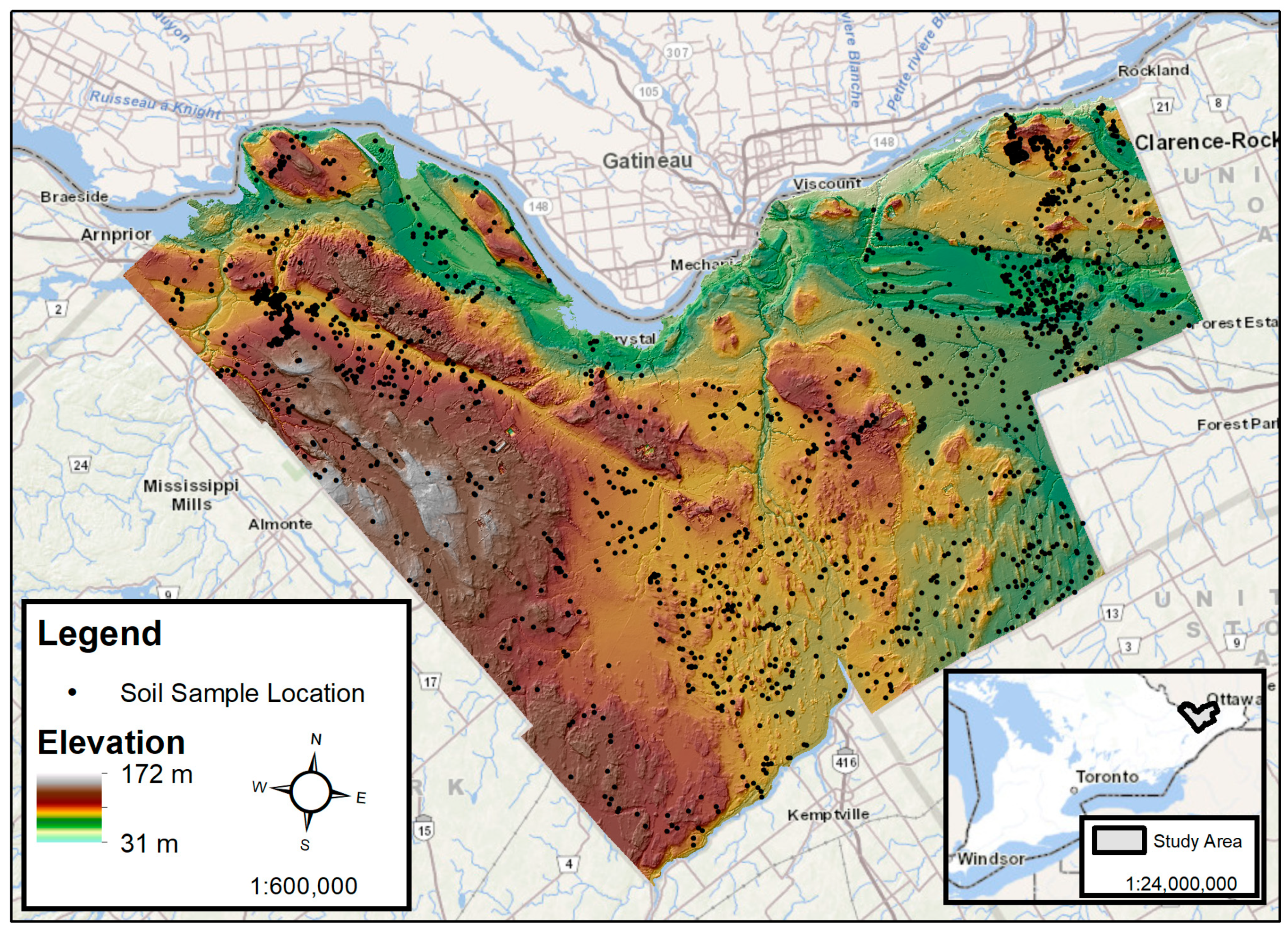
The study area is the City of Ottawa, Canada, which was formed by the amalgamation of Carleton County and the City of Ottawa and is approximately 2790 km2 (Figure 2). The study area is complex both in terms of bedrock geology and surficial (quaternary) geology. Bedrock is mainly of the Paleozoic era, dominated by dolomite and limestone [25]. The southwest portion of the study area is dominated by limestone plains and thin till veneers over bedrock [25]. The central and eastern areas were mostly inundated by the Champlain Sea after continental deglaciation and exhibit various landforms and deposits, such as clay plains, beach ridges, sand deposits, and organic deposits in depressional areas. For a detailed description of the soils, quaternary, and bedrock geology in the study area, see Schut and Wilson [25], Bélanger et al. [26], and MacDonald and Harrison [27].
In total, 1791 soil profiles were described and sampled during the years 2015–2019. Sample locations were identified using a combination of sample points selected using the cLHS algorithm, expert opinion sampling (dense sampling) in two pilot areas evaluated during the early stages of the project (2015), and opportunistic sampling when cLHS locations were inaccessible.
Four soil properties were selected for this study: CEC, clay content, soil pH, and SOC. Clay content was determined using the pipette method with hydrogen peroxide pre-treatment for the removal of organic matter [28]. Cation exchange capacity was determined using the barium chloride extraction method with a buffered 0.5 M solution [29]. Soil pH was determined using the saturated paste method using a 1:1 ratio of soil to 0.01 M calcium chloride solution [30]. Soil organic carbon was determined using the LECO CN828 Elemental analyzer. Total carbon was determined by combusting a soil sample, while inorganic carbon was determined by first ashing a sample at 475 °C for three hours to remove organic carbon and then combusting in the LECO analyzer. Soil organic carbon was calculated as the difference [31].
The equal area quadratic spline [32] approach was used to harmonize each soil profile from the field-described horizon thicknesses to standard depth intervals (0–15 cm, 15–30 cm, 30–60 cm, and 60–100 cm) using the ‘easpline’ function from the ithir package [33]. Only the 0–15 cm depth interval was used for this study.
2.3. Environmental Covariates
A total of 71 continuous covariates and 3 categorical covariates were considered for inclusion in the predictive models (Table 1). Most of the covariates (55) were LiDAR-derived using WhiteboxTools via the whitebox package [34,35] and SAGA-GIS implemented in the rsaga package [36,37] from a digital terrain model at 10-m spatial resolution. Six continuous covariates were gamma-radiometric data [38], while three others were the mean, standard deviation, and maximum of a Google Earth Engine time-series of normalized difference vegetation index (NDVI) images generated from Sentinel-2 imagery representing the growing season (June to September) for a four-year period (2017–2020). The final seven continuous covariates were Euclidean distance fields, which were used to provide spatial context to the predictive model computed in the onsoilsurvey package [39]. Specifically, distance fields were calculated from each raster cell to the northeast, southeast, southwest, and northwest corners of the raster grid, to the maximum X and maximum Y coordinates, and to the middle of the raster grid [40]. The three categorical covariates were quaternary geology (6 classes) [41], bedrock geology (4 classes) [42], and soil order (5 classes) [25,43]. One-hot encoding was used for the categorical covariates [44,45]. Details for each of the covariates are outlined in Table 1.
Covariate reduction is recommended to simplify predictive models and mitigate overfitting caused by the collinearity of the predictors [4,61]. Therefore, the variance inflation factor (VIF) technique was applied to the continuous covariates [62]. The VIF (Equation (1)) calculates how much of the variability from an environmental covariate can be explained by the remaining covariates in the regression model [63]:
where rj2 is the coefficient of determination from fitting a linear regression between the jth independent variable and all other independent variables. The process is run sequentially using the ‘oss.seqVIF’ function in the onsoilsurvey package [39] until only covariates above a selected threshold remain. Thresholds for VIF analysis commonly reported in the literature are five and ten [64,65]. The lower cutoff of five was selected for this analysis to be more conservative and retain fewer covariates, given the large number of covariates at the onset of the analysis. As a result, 44 of the 71 continuous covariates were retained as predictors for modeling, and to these were added the 15 one-hot encoded rasters generated from the categorical predictors. All covariates retained for modeling are in bolded font in Table 1.
2.4. Kriging
Soil property maps (synthetic data) were generated using geostatistical interpolation. Inverse-distance weighted interpolation and universal and ordinary kriging using spherical and exponential models were tested using the gstat package [66]. Ordinary kriging with an exponential model performed the best across all soil properties. As a first step, the point data were thinned in ESRI’s ArcMap software (version 10.8) using the Identical Tool with a minimum spacing set to 500 m. This was conducted to reduce the clustering of sample locations in areas where more intensive field work was conducted and to match the grid resolution at which the kriging model was applied. The remaining points were then evaluated for normal distribution using the ‘transformTukey’ function from the rcompanion package [67], which showed SOC, CEC, and clay as requiring transformation. All three were transformed using a power function: SOC was raised to the power of 0.175, and CEC and clay were each raised to the power of 0.350, based on the output from the ‘transformTukey’ function. The ordinary kriging with exponential models were then fitted to the variograms. Models were then applied to the raster grid of the study area at 500 m spatial resolution. The three transformed soil properties (SOC, CEC, and clay) were then backtransformed to natural values (the inverse of their respective power functions). All four soil property rasters were then resampled to the same 10-m grid of the environmental covariates with a bilinear interpolation.
2.5. Sample Plans and Divergence Metrics
Three sampling algorithms were used to create sample plans: the cLHS [5,68], the FSCS [6], and simple random sampling (SRS). Given the computing constraints of running the cLHS and the FSCS algorithms on the entire study area (~28 million raster cells), an initial test was conducted using SRS to determine an adequate subset of the covariate raster cells that would be representative of the study area. For this test, we computed the DJS [3,69] between sample plans of increasing size and the full covariates (population) until the divergence was minimized and leveled off based on visual inspection (Figure S1). Simple random sampling was then used to draw a random sample (n = 200,000) from the covariates to be used for subsequent analysis.
From the subset created by SRS, an external validation dataset (n = 1000) was selected using the cLHS algorithm and used exclusively for validation of the predictive models. We selected this validation sample size because it represents 25% of the largest calibration sample size, which falls between 20% and 30%, which is a typical range for validation in DSM. From the remaining data (n = 199,000), five independent sample plans were created at each of 25 different sample sizes, ranging from 50 to 4000 samples for each of the three sampling algorithms. Finally, the DJS was computed between each sample plan created and the full data used for creating the sample plans (n = 199,000) using the ‘oss.jsd’ function of the onsoilsurvey package [39]. The overall DJS for a sample plan is computed by calculating the DJS between the sample plan and the population for each environmental covariate individually. Then, the mean DJS of all the covariates is calculated to represent the DJS for the sample plan.
2.6. Predictive Modeling
For each sample plan, the sample locations were used to extract the values of the four target soil properties from the kriging outputs. The sample plans were then used to calibrate a RF model [70], and each model was validated with the external validation dataset. The RF models were trained using the caret package [71], with tuning parameters set to their defaults (ntree = 500 and mtry = # predictors0.5). For each sample size and sampling algorithm, the mean of Lin’s concordance correlation coefficient (CCC) [72] and root mean square error (RMSE) of the five repeated plans were calculated to evaluate model performance.
2.7. Optimal Calibration Sample Size
The goal is to determine an optimal sample size using only the environmental covariates; hence, we first determined the optimal sample size based on the DJS using a rule of diminishing returns [3,19]. The DJS was plotted as a function of sample size, and a cumulative distribution function was calculated from the data. To ensure adequate feature space coverage of the covariates, the location where the cumulative distribution function reaches 95% was used to select the optimal sample size [3,19].
To determine the optimal sample size based on the model performance metrics, the unit-invariant knee technique [73] was selected. This technique identifies the knee point, or elbow point, in the curve fitted through a plot of the performance metrics (CCC and RMSE) as a function of sample size [11]. This is in contrast with the approach described in Saurette et al. [3], where the cumulative distribution function was used to assess sample size based on model performance metrics. However, while Saurette et al. [3] were trying to optimize model performance (i.e., 95% of the cumulative distribution function of CCC or RMSE), in this study we seek to identify the best trade-off between sample size and model performance, or where the return on investment of collecting more samples peaks and additional sampling is no longer justified by the improvements in model performance metrics.
Finally, RF models were trained for each of the four soil properties, with the optimal sample sizes determined from the DJS for each of the three sampling algorithms. Quantile regression forest was applied using the quantregForest package [74,75] to generate 90% prediction interval maps by generating predictions for the 95th and 5th quantiles and subtracting the rasters. While RF estimates the conditional mean of the response variable, quantile regression forest retains the full conditional distribution [74,76] and allows the prediction of any desired quantile around the mean.
3. Results and Discussion
3.1. Soil Properties and Kriged Surfaces
Clay content ranged from 0 to 83% throughout the study area (Table 2). This wide range of values is expected based on the complex quaternary geology of the site, which contains marine clay plains and beach ridges from the intrusion of the Champlain Sea during deglaciation, sandy and gravelly glaciofluvial outwash deposits, and morainal deposits. The predicted surfaces of the four target soil properties are provided in Figure 3. Cation exchange capacity (0.25 to 103.70 cmol+/kg) and soil pH (3.3 to 7.6) generally follow the same spatial patterns as the clay content, where coarser soils are associated with more acidic pH and lower cation exchange capacity, while fine-textured soils tend to have both higher pH and cation exchange capacity (Figure 3).
All four properties were modeled with universal kriging and exponential models. The variograms are shown in Figure S2, and the model parameters are in Table 3. Cation exchange capacity and SOC had similar ranges (5553 m and 5215 m, respectively). Soil pH had the largest range, 11,331 m, highlighting the major bedrock and surficial deposits in the study area. The southern half of the study area exhibits high pH values, and these areas are aligned with limestone bedrock with thin drift (till) in the southwest and morainal deposit in the southeast [26,27]. The area of lower pH in the northwest is aligned with an acidic Precambrian bedrock outcrop, while the northeast corner is associated with sandy outwash materials [25,27].
3.2. Optimal Sample Size—Divergence Metrics
The DJS for all three sampling algorithms (cLHS, SRS, and FSCS) showed a very similar exponential decay as a function of increasing sample size (Figure 4). The exponential decrease is expected since, as sample size increases, more data is selected to approximate the probability distribution of the population (covariates) with the sample plan. The maximum DJS for all three sampling algorithms was 0.33 at the smallest sample size tested, which was 50 samples. The DJS is bound between 0 and 1, which indicates that with as few as 50 samples, the sampling algorithms were able to approximate the covariates successfully. The exponential decay functions fitted with non-linear least squares regression tend to level off at approximately 2000 sample points for all three algorithms, and all three fitted curves are slightly above the true values of the DJS (Figure 4). Something interesting about this result is that the cLHS and the FSCS algorithms did not have an advantage over SRS at the smaller sample sizes (i.e., smaller values of DJS), given that these algorithms are designed to sample in feature space and are regarded as superior to SRS in many studies [14,77,78,79]. Finally, when using a cumulative distribution function of the DJS to determine the optimal sample size, all three algorithms determined a similar optimal size (865, 869, and 874 samples for the cLHS, SRS, and FSCS, respectively). The final sample sizes from the three algorithms being quite similar is not unexpected. As sample size increases, the likelihood of approximating the cumulative distribution function increases, and at a given point (e.g., optimal size), additional samples no longer improve the sample plan.
3.3. Optimal Sample Size—Learning Curves
The model performance metrics as a function of sample size (learning curves) from the external validation of the RF models are provided in Figure 5 for CEC. Plots for clay, pH, and SOC are provided in Supplementary Materials (Figures S3–S5). Concordance increased quickly, while RMSE decreased quickly, as a function of sample size. This aligns with similar studies that show model performance metrics improve quickly at smaller sample sizes and then gradually level off [12,20]. In general, the sample plans selected with cLHS and FSCS outperformed those created with SRS in terms of both performance metrics at smaller sample sizes. As the sample size increased, the difference in the performance metrics decreased and became less significant. The diminishing height of the boxplots and whiskers with increasing sample size demonstrated the higher variability of the sample plans at smaller sample sizes (Figure 5), a trend that was observed in similar studies [11,80].
The optimal sample size, as identified using the unit invariant knee, varied by soil property and by sampling algorithm (Table 4). For CEC, the FSCS sampling reached the optimum at 800 samples (0.29 samples/km2, CCC = 0.74, RMSE = 3.03), while the cLHS optimized sample size was 900 samples (0.32 samples/km2, CCC = 0.76, RMSE = 2.93) and the SRS optimized at 1000 samples (0.36 samples/km2, CCC = 0.76, RMSE = 2.95). CEC was the only soil property where the optimal sample size was identical using both CCC and RMSE. Despite the CCC and RMSE being slightly better using the cLHS and SRS plans, the difference would hardly justify collecting an additional 100–200 samples. For clay content, the FSCS resulted in the largest optimal sample sizes based on CCC (900 samples, CCC = 0.66) and RMSE (1400 samples, 0.50 samples/km2, RMSE = 4.37%), while the cLHS and SRS plans resulted in much smaller optimal sample sizes (600–700 samples, or 0.22 to 0.25 samples/km2) but with similar performance metrics (CCC = 0.65 and RMSE = 4.76 for cLHS and CCC = 0.62 and RMSE = 4.89 for SRS). For pH, the optimal sample sizes ranged from 500 to 900 samples (0.18 to 0.32 samples/km2) based on the CCC (0.89) and RMSE (0.18) using the cLHS, and from 500 samples based on the CCC (0.88) to 800 samples based on the RMSE (0.19) for the SRS (0.18 to 0.29 samples/km2). For the FSCS, the optimal sample sizes based on the CCC (0.90) and RMSE (0.20) were both 700 (or 0.25 samples/km2). Finally, the optimal sample sizes based on both the CCC and RMSE for the SOC predictions were 1000 when using the cLHS (0.36 samples/km2, CCC = 0.66, RMSE = 0.32) and 1400 (0.50 samples/km2, CCC = 0.71, RMSE = 0.30) when using the FSCS. The optimal sample size for SOC when using SRS ranged between 1200 samples (0.43 samples/km2, CCC = 0.68) and 1600 (0.57 samples/km2, RMSE = 0.28). The sampling density for optimizing the predictions of SOC is significantly higher than that reported by Shao et al. [81], who found rapid and moderate improvement in model performance up to a sampling density of 0.09 samples/km2 and 0.24 samples/km2, respectively, yet significantly lower than the sampling densities reported by Safaee et al. [82], who reported improved model performance up to a sample density of 12 samples/km2. The optimal calibration sample sizes required to predict the four different soil properties are quite variable, especially in the case of SOC, and likely a result of a combination of factors, including the spatial variability of the response variable and the relationship between the dependent variable and the explanatory covariates. Safaee et al. [82] attributed poorer model performance in predicting SOM to the intensity and complexity of land use management and the masking effect this had on the relationship of SOM with landscape properties.
Since DSM projects are often designed with the goal of predicting several soil properties, it is useful to summarize the size of the optimal sample plans by soil property and by sampling algorithm to better understand the implications of these factors when designing a project. Summarizing (median) by soil property, the optimal sample size increased in the order of soil pH (700) = clay (700) < CEC (900) < SOC (1300). As stated above, this is likely linked to the relationship of the soil properties to the explanatory covariates. Summarizing by sampling algorithm across all soil properties, the optimal sample size increased in the order FSCS (850) < cLHS (900) = SRS (900), highlighting how little difference there is in the optimal sample size when using these three techniques. In fact, the median CCC associated with these optimal sample sizes across all soil properties was 0.73 for FSCS, 0.72 for SRS, and 0.71 for cLHS, again showing there is little difference between the performance of the models trained using sampling plans developed from the three sampling algorithms. Numerous studies have observed this same trend, where model performance is more dependent on the size of the calibration dataset, and less sensitive to the sampling algorithm used to create the sample plan. For example, Bouasria et al. [14] showed minimal difference in RF model performance when comparing sample plans developed from cLHS and SRS to predict aboveground biomass, and Loiseau et al. [83] noted no substantial difference in quantile RF predictions of sand, silt, and clay between SRS and cLHS sample plans. Schmidinger et al. [12] noted higher RMSE and lower CCC with SRS compared to cLHS and FSCS at smaller sample sizes, whereas the differences decreased as sample sizes increased until all three sampling designs showed the same performance. To the contrary, Ma et al. [82] showed that the overall accuracy of soil class prediction with RF was better with FSCS than it was with cLHS and SRS. In this study, whether CCC or RMSE was used to calculate the optimal sample size with the unit invariant knee, the range was the same as for the sampling algorithms (CCC = 850, RMSE = 900).
3.4. Optimal Sample Size—Overall
The optimal sample sizes for each algorithm based on the DJS computed from the covariates (865, 874, and 869 samples for the cLHS, FSCS, and SRS, respectively) are remarkably close to the optimal sample sizes based on model performance (900, 900, and 850 samples for the cLHS, SRS, and FSCS, respectively). This agrees with the findings of Saurette et al. [3], who confirmed this using a field-scale example of total organic carbon modeling for a 26-ha field in Ontario. This finding suggests two further outcomes: first, that divergence metrics are stable and reliable for estimating the optimal sample size for DSM, and second, that the use of divergence metrics for determining the optimal sample size is not affected by the size of the study area. The reason for this is that the DJS relies only on the probability distribution functions of the covariates; therefore, it is not sensitive to the overall size of the total pool of potential sample locations (i.e., total raster cells in the study area). The optimal sample sizes are equivalent to 0.31–0.32 inspections/km2, which is slightly higher than the average sampling intensity reported in Wadoux et al. [4] of 0.24 inspections/km2, and which is closer to the low end of the range for sampling intensity in the conventional Canadian SIL3 soil survey (0.1–1 inspections/km2).
3.5. Final Random Forest Predictions and Uncertainty
The optimal sample sizes for each sampling algorithm (based on the DJS) were then used to create a final calibration dataset to train RF models. The predictions for the four target soil properties using the cLHS sampling algorithm are shown in Figure 6, while those for FSCS and SRS are shown in Figures S6 and S7. When compared to the surfaces created by kriging (Figure 3), which were the synthetic data used for the sampling plan development, the RF predictions (Figure 6) exhibit the same spatial patterns across the study area. This demonstrates that the RF models calibrated with the optimal sample sizes determined using the DJS were successful in predicting the spatial variability of each of the target soil properties. In all cases, the maps generated from the RF models using the covariates generally have sharper boundaries that are tied to the underlying covariates. For example, in the northeast corner of the study area, a large outwash area is more discernible in the RF outputs than in the kriging outputs. These observations are consistent with the outputs of the RF models, for which FSCS and SRS were used to draw the sample plan.
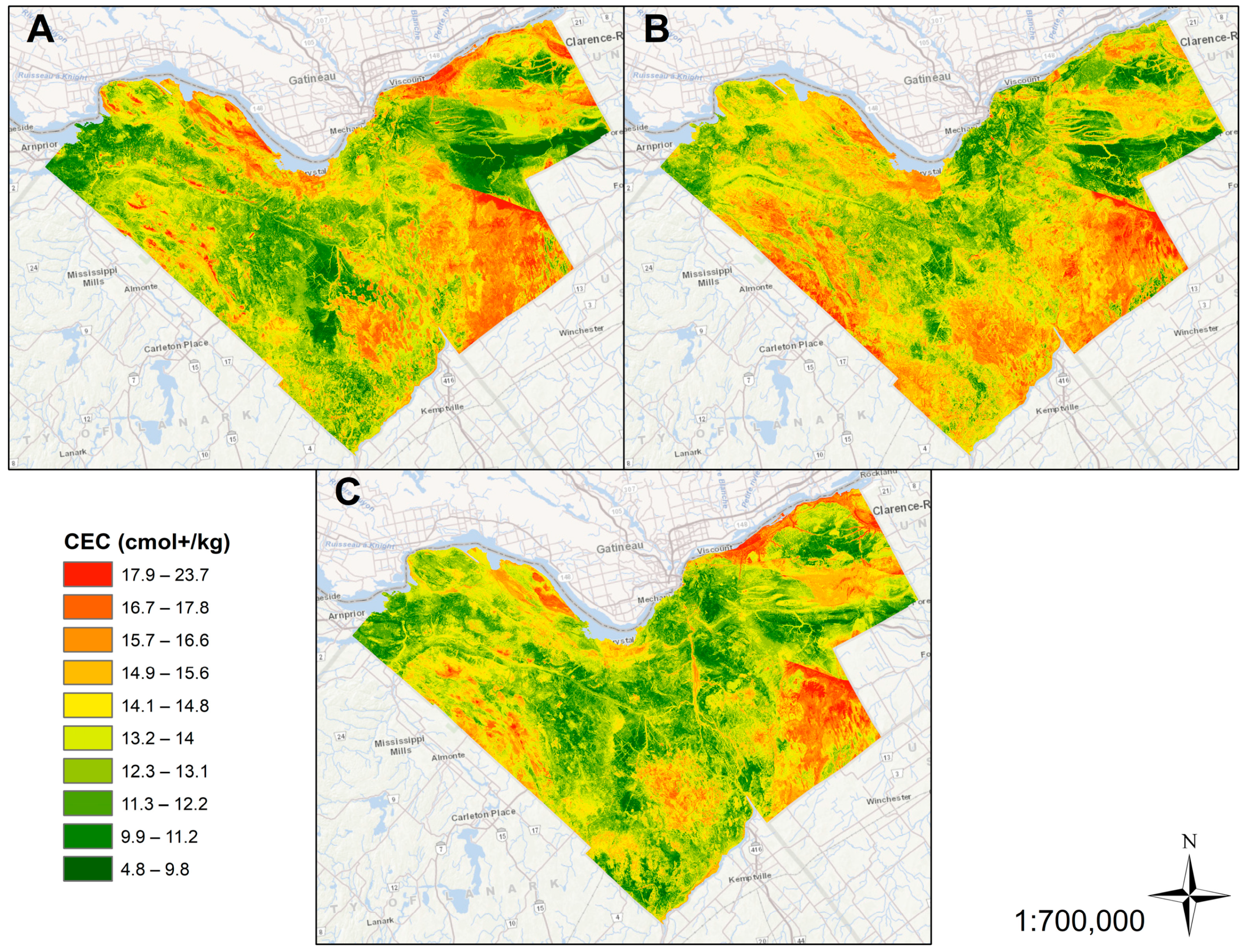
In general, the uncertainty maps show similar spatial patterns, regardless of the sampling algorithm used to select the optimal sample plan (Figure 7). The prediction interval maps for CEC are provided in Figure 7, while the maps for clay, pH, and SOC are provided in the Supplementary Materials (Figures S8–S10). The 90% prediction interval for CEC ranged from 5.8 to 23.7 cmol+/kg. Uncertainty was highest in the southeast corner of the map for all three sampling algorithms. This portion of the map has fine to moderately fine sediments of varying thickness overlying loamy, calcareous glacial till; the complex materials may contribute to the uncertainty. The prediction interval maps for the cLHS (Figure 7A) and the SRS (Figure 7C) sampling algorithms show higher uncertainty than the FSCS (Figure 7B) in the northern border of the map, which follows the Ottawa River. The median prediction interval widths were 13.5, 14.6, and 13.3 cmol+/kg for the cLHS, FCS, and SRS sampling algorithms, respectively. Based on the visual review and the median prediction intervals, there were no important differences. These trends are also apparent in the prediction interval maps for the other three soil properties (Figures S8–S10). It should be noted, however, that several studies have demonstrated that the use of ensemble modeling approaches can be leveraged to balance the outcomes of different machine learning algorithms [84,85,86]. Given some localized differences in the uncertainty of the predictions, an ensemble approach may be beneficial for this study area; however, this was out of the scope of the current research.
Overall, the investigation has yielded pivotal insights into the pedological nuances of determining optimal sample sizes through the lens of divergence metrics, notably the DJS. We found that even minimal sample sizes could effectively approximate the distributions of environmental covariates, challenging the traditional emphasis on specific feature space sampling methods. This insight led us to understand that the choice of sampling algorithm—whether cLHS, FSCS, or SRS—had minimal impact on the model’s performance at smaller sample sizes. Instead, we recognized that the optimal sample size is intricately linked to the spatial variability of soil properties and their interaction with DSM model performance. Thus, this study significantly advanced the field of DSM, particularly the strategic determination of sample sizes. We observed that integrating pedological expertise with advanced statistical methods can be crucial for accurately capturing the complexity of soil landscapes. Our work underscores the need for a nuanced approach to DSM, where pedologists can use divergence metrics to refine sampling strategies, thereby enhancing the accuracy of soil property predictions. This methodology not only propels pedological science forward but also has implications for land management practices. It provides a scientifically robust basis for decisions impacting soil health, agricultural productivity, and environmental sustainability. By marrying conventional pedology with modern computational techniques, we pave the way for future soil science endeavors to tackle the challenges of sustainable land use and conservation more effectively.
In this study, we examined the optimal sample size for a single depth interval, whereas in many DSM projects, soil properties are predicted for several standardized depth intervals [87,88,89]. The impact of considering additional depths is not clear. Studies have shown that model performance deteriorates with depth and have attributed this to a weakened relationship between the environmental covariates and the soil properties at depth [89]. This is certainly valid given the predominance of terrain derivatives and remotely sensed data used to generate environmental covariates in DSM, which reflect the surface properties of the study area. Soils generally become more homogeneous with depth as the parent material is approached, and the effect of the interaction of soil with the surface environment decreases (e.g., less organic matter incorporation, less water infiltration, etc.). These two factors—poorer model performance at depth and loss of a relationship between covariates and soil properties—suggest that additional sampling may not enhance DSM models for depth intervals below the surface. Despite this, the sampling requirements for several depth intervals may influence the optimal calibration sample size, and this should be explored.
4. Conclusions
In our research, we explored the effectiveness of the DJS in identifying the optimal calibration sample size for mapping four soil properties across a 2790 km2 area. We applied this method alongside three prevalent sampling strategies—cLHS, FSCS, and SRS—to validate the robustness of the DJS-derived sample size estimates. Through the calibration of RF models and the assessment of model performance against sample size using CCC and RMSE metrics, we pinpointed the optimal balance as indicated by the unit invariant knee. Our findings reveal a remarkable consistency in optimal calibration sample sizes across the sampling strategies (865 for cLHS, 874 for FSCS, and 869 for SRS), closely aligning with the sample sizes derived from model performance metrics (850–900 samples) for the soil properties studied. This consistency extends the work of Saurette et al. [3], scaling the application from a field-scale study to a significantly larger area, thereby confirming the utility of DJS in broader DSM contexts. Our conclusion is clear: the DJS emerges as a dependable metric for determining optimal calibration sample sizes in DSM, warranting its inclusion among the essential tools for DSM sampling design, thereby enhancing the precision and reliability of soil property mapping at scale.
Supplementary Materials
The following supporting information can be downloaded at: https://www.mdpi.com/article/10.3390/land13030365/s1, Figure S1. Jensen–Shannon Divergence (DJS) as a function of sample size for the 44 continuous covariates retained after the variance inflation factor covariate reduction. Sample plans were generated from the full covariate rasters using simple random sampling. Subplot A shows the DJS across all sample sizes, while subplot B highlights the DJS for sample sizes ≥6400. Codes for the covariates are provided for completeness despite the overlap, which prevents identifying them individually. Figure S2. Experimental semivariograms with fitted exponential model (solid line) for the four target soil properties: cation exchange capacity (A), clay content (B), soil pH (C), and soil organic carbon (D). Note that the kriging was performed on transformed values for cation exchange capacity, clay, and soil organic carbon; therefore, the semivariances presented along the ordinate are transformed units. Figure S3. Change in the concordance and root mean square error (RMSE) with increasing sample size from the external validation of the random forest models trained with sample plans developed using conditioned Latin hypercube sampling (cLHS), feature space coverage sampling (FSCS), and simple random sampling (SRS) for clay content. The solid (orange) vertical line, dashed (blue) vertical line, and dotted (green) vertical line identify the optimal sample size based on the unit invariant knee for the cLHS, FSCS, and SRS sampling algorithms, respectively. Figure S4. Change in the concordance and root mean square error (RMSE) with increasing sample size from the external validation of the random forest models trained with sample plans developed using conditioned Latin hypercube sampling (cLHS), feature space coverage sampling (FSCS), and simple random sampling (SRS) for soil pH. The solid (orange) vertical line, dashed (blue) vertical line, and dotted (green) vertical line identify the optimal sample size based on the unit invariant knee for the cLHS, FSCS and SRS sampling algorithms, respectively. Figure S5. Change in the concordance and root mean square error (RMSE) with increasing sample size from the external validation of the random forest models trained with sample plans developed using conditioned Latin hypercube sampling (cLHS), feature space coverage sampling (FSCS), and simple random sampling (SRS) for soil organic carbon. The solid (orange) vertical line, dashed (blue) vertical line, and dotted (green) vertical line identify the optimal sample size based on the unit invariant knee for the cLHS, FSCS, and SRS sampling algorithms, respectively. Figure S6. Random forest predictions of (A) cation exchange capacity (CEC), (B) clay content, (C) soil pH, and (D) soil organic carbon (SOC) for the Ottawa Study area using a sample plan created with feature space coverage sampling and the overall optimal sample size of 874 sample locations. Figure S7. Random forest predictions of (A) cation exchange capacity (CEC), (B) clay content, (C) soil pH, and (D) soil organic carbon (SOC) for the Ottawa Study area using a sample plan created with simple random sampling and the overall optimal sample size of 869 sample locations. Figure S8. Prediction interval maps (90%) for clay content generated using quantile regression forest for the optimal sample sizes based on the Jenson-Shannon Divergence for conditioned Latin hypercube sampling (A), feature space coverage sampling (B), and simple random sampling (C) algorithms. Figure S9. Prediction interval maps (90%) for soil pH generated using quantile regression forest for the optimal sample sizes based on the Jenson-Shannon Divergence for conditioned Latin hypercube sampling (A), feature space coverage sampling (B), and simple random sampling (C) algorithms. Figure S10. Prediction interval maps (90%) for soil organic carbon (SOC) generated using quantile regression forest for the optimal sample sizes based on the Jenson-Shannon Divergence for conditioned Latin hypercube sampling (A), feature space coverage sampling (B), and simple random sampling (C) algorithms.
Author Contributions
Conceptualization, D.D.S. and A.B.; Software, D.D.S.; Writing—Original Draft, D.D.S.; Writing—Review and Editing, D.D.S., A.A.B., R.J.H., A.W.G., and A.B.; Supervision—A.B. All authors have read and agreed to the published version of the manuscript.
Funding
This research was funded by the Natural Science and Engineering Research Council (NSERC) of Canada, which supported and funded this project through an NSERC Postgraduate Scholarship—Doctoral (PGS-D) to D.D.S. and through grant RGPIN-2020-05017 to A.B.
Data Availability Statement
The data presented in this study are available on request from the corresponding author. The datasets presented in this article are not readily available because the data are part of an ongoing study. Requests to access the datasets should be directed to Daniel Saurette at [email protected].
Acknowledgments
The authors would like to thank the Ontario Ministry of Agriculture, Food and Rural Affairs for contributing the data collected in the Ottawa Soil Survey project, without which this research would not be possible. The authors also thank the field pedologists, interns, and summer students for their considerable efforts in the execution of the field program.
Conflicts of Interest
The authors declare no conflicts of interest.
References
- Mapping Systems Working Group. A Soil Mapping System for Canada: Revised.; Land Resource Research Institute, Research Branch, Agriculture Canada: Ottawa, ON, Canada, 1981; p. 94. [Google Scholar]
- Expert Committee on Soil Survey. Soil Survey Handook; Coen, G.M., Ed.; Land Resource Research Centre, Research Branch, Agriculture Canada: Ottawa, ON, Canada, 1987; Volume 1, ISBN 0-662-15374-X. [Google Scholar]
- Saurette, D.D.; Heck, R.J.; Gillespie, A.W.; Berg, A.A.; Biswas, A. Divergence Metrics for Determining Optimal Training Sample Size in Digital Soil Mapping. Geoderma 2023, 436, 116553. [Google Scholar] [CrossRef]
- Wadoux, A.M.J.-C.; Minasny, B.; McBratney, A.B. Machine Learning for Digital Soil Mapping: Applications, Challenges and Suggested Solutions. Earth-Sci. Rev. 2020, 210, 103359. [Google Scholar] [CrossRef]
- Minasny, B.; McBratney, A.B. A Conditioned Latin Hypercube Method for Sampling in the Presence of Ancillary Information. Comput. Geosci. 2006, 32, 1378–1388. [Google Scholar] [CrossRef]
- Brus, D.J. Sampling for Digital Soil Mapping: A Tutorial Supported by R Scripts. Geoderma 2019, 338, 464–480. [Google Scholar] [CrossRef]
- Biswas, A.; Zhang, Y. Sampling Designs for Validating Digital Soil Maps: A Review. Pedosphere 2018, 28, 1–15. [Google Scholar] [CrossRef]
- Tiedeman, K.; Chamberlin, J.; Kosmowski, F.; Ayalew, H.; Sida, T.; Hijmans, R.J. Field Data Collection Methods Strongly Affect Satellite-Based Crop Yield Estimation. Remote Sens. 2022, 14, 1995. [Google Scholar] [CrossRef]
- Jeong, J.H.; Resop, J.P.; Mueller, N.D.; Fleisher, D.H.; Yun, K.; Butler, E.E.; Timlin, D.J.; Shim, K.-M.; Gerber, J.S.; Reddy, V.R.; et al. Random Forests for Global and Regional Crop Yield Predictions. PLoS ONE 2016, 11, e0156571. [Google Scholar] [CrossRef]
- Castro-Franco, M.; Costa, J.L.; Peralta, N.; Aparicio, V. Prediction of Soil Properties at Farm Scale Using a Model-Based Soil Sampling Scheme and Random Forest. Soil Sci. 2015, 180, 74–85. [Google Scholar] [CrossRef]
- Saurette, D.D.; Berg, A.A.; Laamrani, A.; Heck, R.J.; Gillespie, A.W.; Voroney, P.; Biswas, A. Effects of Sample Size and Covariate Resolution on Field-Scale Predictive Digital Mapping of Soil Carbon. Geoderma 2022, 425, 116054. [Google Scholar] [CrossRef]
- Schmidinger, J.; Schröter, I.; Bönecke, E.; Gebbers, R.; Ruehlmann, J.; Kramer, E.; Mulder, V.L.; Heuvelink, G.B.M.; Vogel, S. Effect of Training Sample Size, Sampling Design and Prediction Model on Soil Mapping with Proximal Sensing Data for Precision Liming. Precis. Agric. 2024. [Google Scholar] [CrossRef]
- Whelan, B.M.; McBratney, A.B.; Viscarra Rossel, R.A. Spatial Prediction for Precision Agriculture. In Proceedings of the Third International Conference on Precision Agriculture, Minneapolis, MN, USA, 23–26 June 1996; ASA, CSSA, and SSSA Books. pp. 331–342, ISBN 978-0-89118-257-3. [Google Scholar]
- Bouasria, A.; Bouslihim, Y.; Gupta, S.; Taghizadeh-Mehrjardi, R.; Hengl, T. Predictive Performance of Machine Learning Model with Varying Sampling Designs, Sample Sizes, and Spatial Extents. Ecol. Inform. 2023, 78, 102294. [Google Scholar] [CrossRef]
- Wisz, M.S.; Hijmans, R.J.; Li, J.; Peterson, A.T.; Graham, C.H.; Guisan, A.; NCEAS Predicting Species Distributions Working Group. Effects of Sample Size on the Performance of Species Distribution Models. Divers. Distrib. 2008, 14, 763–773. [Google Scholar] [CrossRef]
- Ng, W.; Minasny, B.; Malone, B.; Filippi, P. In Search of an Optimum Sampling Algorithm for Prediction of Soil Properties from Infrared Spectra. PeerJ 2018, 6, 5722. [Google Scholar] [CrossRef]
- Ng, W.; Minasny, B.; Mendes, W.D.S.; Demattê, J.A.M. The Influence of Training Sample Size on the Accuracy of Deep Learning Models for the Prediction of Soil Properties with Near-Infrared Spectroscopy Data. SOIL 2020, 6, 565–578. [Google Scholar] [CrossRef]
- Chen, S.; Arrouays, D.; Leatitia Mulder, V.; Poggio, L.; Minasny, B.; Roudier, P.; Libohova, Z.; Lagacherie, P.; Shi, Z.; Hannam, J.; et al. Digital Mapping of GlobalSoilMap Soil Properties at a Broad Scale: A Review. Geoderma 2022, 409, 115567. [Google Scholar] [CrossRef]
- Malone, B.P.; Minansy, B.; Brungard, C. Some Methods to Improve the Utility of Conditioned Latin Hypercube Sampling. PeerJ 2019, 7, e6451. [Google Scholar] [CrossRef] [PubMed]
- Khan, A.; Aitkenhead, M.; Stark, C.R.; Ehsan Jorat, M. Optimal Sampling Using Conditioned Latin Hypercube for Digital Soil Mapping: An Approach Using Bhattacharyya Distance. Geoderma 2023, 439, 116660. [Google Scholar] [CrossRef]
- Stumpf, F.; Schmidt, K.; Behrens, T.; Schönbrodt-Stitt, S.; Buzzo, G.; Dumperth, C.; Wadoux, A.; Xiang, W.; Scholten, T. Incorporating Limited Field Operability and Legacy Soil Samples in a Hypercube Sampling Design for Digital Soil Mapping. J. Plant Nutr. Soil Sci. 2016, 179, 499–509. [Google Scholar] [CrossRef]
- Brungard, C.W.; Boettinger, J.L. Conditioned Latin Hypercube Sampling: Optimal Sample Size for Digital Soil Mapping of Arid Rangelands in Utah, USA. In Digital Soil Mapping: Bridging Research, Environmental Application, and Operation; Boettinger, J.L., Howell, D.W., Moore, A.C., Hartemink, A.E., Kienast-Brown, S., Eds.; Springer: Dordrecht, The Netherlands, 2010; pp. 67–75. ISBN 978-90-481-8863-5. [Google Scholar]
- Garrido, A. About Some Properties of the Kullback-Leibler Divergence. Adv. Model. Optim. 2009, 11, 8. [Google Scholar]
- McBratney, A.; Mendonça Santos, M.L.; Minasny, B. On Digital Soil Mapping. Geoderma 2003, 117, 3–52. [Google Scholar] [CrossRef]
- Schut, L.W.; Wilson, E.A. The Soils of the Regional Municipality of Ottawa-Carleton; Ontario Institute of Pedology, Research Branch, Agriculture and Agri-Food Canada, Ontario Ministry of Agriculture and Food, Department of Land Resource Science, University of Guelph: Guelph, ON, Canada, 1987; p. 118. [Google Scholar]
- Bélanger, J.R.; Moore, A.; Prégent, A.; Richard, H. Surficial Geology—Ottawa, Ontario-Quebec (31G/5); Geological Survey of Canada: Ottawa, ON, Canada, 1995. [Google Scholar]
- MacDonald, G.; Harrison, J.E. Generalized Bedrock Geology, Ottawa-Hull, Ontario and Quebec; Government of Canada: Matane, QC, Canada, 1979. [Google Scholar]
- Sheldrick, B.H.; Wang, C. Particle Size Distribution. In Soil Sampling and Methods of Analysis; Lewis Publishers: Boca Raton, FL, USA; Canadian Society of Soil Science: Pinawa, MB, Canada, 1993; pp. 499–507. [Google Scholar]
- Rhoades, J.D. Cation Exchange Capacity. In Methods of Soil Analysis. Part 2. Chemical and Microbiological Properties; Page, A.L., Miller, R.H., Keeney, D.R., Eds.; American Society of Agronomy, Inc. Soil Science Society of America, Inc.: Madison, WI, USA, 1982; pp. 149–157. ISBN 978-0-89118-977-0. [Google Scholar]
- McKeague, J.A. (Ed.) Manual on Soil Sampling and Methods of Analysis, 2nd ed.; Subcommittee on Methods of Analysis of the Canada Soil Survey Committee, Canadian Society of Soil Science: Pinawa, MB, Canada, 1978. [Google Scholar]
- Kalembasa, S.J.; Jenkinson, D.S. A Comparative Study of Titrimetric and Gravimetric Methods for the Determination of Organic Carbon in Soil. J. Sci. Food Agric. 1973, 24, 1085–1090. [Google Scholar] [CrossRef]
- Bishop, T.F.A.; McBratney, A.B.; Laslett, G.M. Modelling Soil Attribute Depth Functions with Equal-Area Quadratic Smoothing Splines. Geoderma 1999, 91, 27–45. [Google Scholar] [CrossRef]
- Malone, B.P. Ithir: Soil Data and Some Useful Associated Functions. R Package Version 1.0. 2018. Available online: https://bitbucket.org/brendo1001/ithir/src/master/ (accessed on 15 February 2024).
- Lindsay, J. WhiteboxTools User Manual; University of Guelph: Guelph, ON, Canada, 2018; p. 234. [Google Scholar]
- Wu, Q.; Brown, A. Whitebox: “WhiteboxTools” R Frontend. R Package Version 2.2.0. 2022. Available online: https://CRAN.R-project.org/package=whitebox (accessed on 15 February 2024).
- Brenning, A.; Bangs, D.; Becker, M. RSAGA: SAGA Geoprocessing and Terrain Analysis. R Package Version 1.4.0. 2022. Available online: https://CRAN.R-project.org/package=RSAGA (accessed on 15 February 2024).
- Conrad, O.; Bechtel, B.; Bock, M.; Dietrich, H.; Fischer, E.; Gerlitz, L.; Wehberg, J.; Winchmann, V.; Böhner, J. System for Automated Geoscientific Analyses (SAGA) v.2.1.4. Geosci. Model Dev. 2015, 8, 1991–2007. [Google Scholar] [CrossRef]
- Natural Resources Canada. Geoscience Data Repository for Geophysical Data. In Magnetic-Radiometric-EM Datasets; Natural Resources Canada: Ottawa, ON, Canada, 2019. [Google Scholar]
- Saurette, D.D. Onsoilsurvey: Making PDSM in Ontario Better. R package version 0.0. 0.9000. 2021. Available online: https://github.com/newdale/onsoilsurvey (accessed on 15 February 2024).
- Behrens, T.; Schmidt, K.; Rossel, R.A.V.; Gries, P.; Scholten, T.; MacMillan, R.A. Spatial Modelling with Euclidean Distance Fields and Machine Learning. Eur. J. Soil Sci. 2018, 69, 757–770. [Google Scholar] [CrossRef]
- Ontario Geological Survey. Surficial Geology of Southern Ontario. Miscellaneous Release—Data-128-REV. 2010. Available online: https://www.geologyontario.mndm.gov.on.ca/mndmfiles/pub/data/imaging/MRD128-REV//MRD128-REV_metadata.pdf? (accessed on 15 February 2024).
- Ontario Geological Survey. 1:250,000 Scale Bedrock Geology of Ontario. Miscellaneous Release—DATA 126—Revision 1. 2011. Available online: https://www.geologyontario.mndm.gov.on.ca/mndmfiles/pub/data/records/MRD126-REV1.html (accessed on 15 February 2024).
- Ontario Ministry of Agriculture, Food and Rural Affairs Ontario Soil Survey Complex. 2019. Available online: https://www.arcgis.com/home/item.html?id=a0eec61f72334bf7b4fc85d2f67456bd (accessed on 15 February 2024).
- Kuhn, M.; Johnson, K. Applied Predictive Modeling; Springer: New York, NY, USA, 2013; ISBN 978-1-4614-6848-6. [Google Scholar]
- Kuhn, M. The Caret Package. Available online: https://topepo.github.io/caret/ (accessed on 1 September 2023).
- Freeman, T.G. Calculating Catchment Area with Divergent Flow Based on a Regular Grid. Comput. Geosci. 1991, 17, 413–422. [Google Scholar] [CrossRef]
- Koethe, R.; Lehmeier, F. SARA—System Zur Automatischen Relief-Analyse, User Manual, 2nd ed.; University of Goettingen: Göttingen, Germany, 1996. [Google Scholar]
- Zevenbergen, L.W.; Thorne, C.R. Quantitative Analysis of Land Surface Topography. Process. Landf. 1987, 12, 47–56. [Google Scholar] [CrossRef]
- Desmet, P.J.J.; Govers, G. A GIS Procedure for Automatically Calculating the USLE LS Factor on Topographical;Ly Complex Landscape Units. J. Soil Water Conserv. 1996, 51, 427–433. [Google Scholar]
- Gallant, J.C.; Dowling, T.I. A Multiresolution Index of Valley Bottom Flatness for Mapping Depressional Areas. Water Resour. Res. 2003, 39, 1347–1359. [Google Scholar] [CrossRef]
- Böhner, J.; Selige, T. Spatial Prediction of Soil Attributes Using Terrain Analysis and Climate Regionalisation. In SAGA—Analysis and Modelling Aplications; Boehner, J., McCloy, K.R., Strobl, J., Eds.; Goettinger Geographische Abhandlungen: Göttingen, Germany, 2006; Volume 115, pp. 13–28. [Google Scholar]
- Weiss, A. Topographic Position and Landforms Analysis. In Proceedings of the ESRI User Conference, San Diego, CA, USA, 9–13 July 2001. [Google Scholar]
- McKenzie, N.; Gessler, P.; Ryan, P.; O”Connell, D. The Role of Terrain Analysis in Soil Mapping. In Terrain Analysis: Principals and Applications; Wilson, J.P., Gallant, J.C., Eds.; John Wiley and Sons Inc.: Hoboken, NJ, USA, 2000. [Google Scholar]
- Moore, I.D.; Grayson, R.B.; Lasdon, A.R. Digital Terrain Modelling: A Review of Hydrological, Geomorphological, and Biological Applications. Hydrol. Process. 1991, 5, 3–30. [Google Scholar] [CrossRef]
- Böhner, J.; Antonic, O. Land-Surface Parameters Specific to Topo-Climatology. In Geomorphometry—Concepts, Software, Aplications. Developments in Soil Science.; Hengl, T., Reuter, H., Eds.; Elsevier: Amsterdam, The Netherlands, 2009; Volume 33, pp. 195–226. [Google Scholar]
- Böhner, J.; Koethe, R.; Conrad, O.; Gross, J.; Ringeler, A.; Selige, T. Soil Regionalisation by Means of Terrain Analysis and Process Parameterisation. In Soil Classification 2001; European Soil Bureau: Luxembourg, 2002; pp. 213–222. [Google Scholar]
- Guisan, A.; Weiss, S.B.; Weiss, A.D. GLM versus CCA Spatial Modeling of Plant Species Distribution. Plant Ecol. 1999, 143, 107–122. [Google Scholar] [CrossRef]
- Riley, S.J.; De Gloria, S.D.; Elliot, R. A Terrain Ruggedness That Quantifies Topographic Heterogeneity. Intermt. J. Sci. 1999, 5, 23–27. [Google Scholar]
- Beven, K.J.; Kirkby, M.J. A Physically-Based Variable Contributing Area Model of Basin Hydrology. Hydrol. Sci. Bull. 1979, 24, 43–69. [Google Scholar] [CrossRef]
- Rodriguez, F.; Maire, E.; Courjault-Rad’e, P.; Darrozes, J. The Black Top Hat Function to a DEM: A Tool to Estimate Recent Incision in a Mountainous Watershed. Geophys. Res. Lett. 2002, 29, 9-1–9-4. [Google Scholar] [CrossRef]
- Ferhatoglu, C.; Miller, B.A. Choosing Feature Selection Methods for Spatial Modeling of Soil Fertility Properties at the Field Scale. In Proceedings of the 30th International Conference on Advances in Geographic Information Systems, Seattle, WA, USA, 1–4 November 2022; Association for Computing Machinery: New York, NY, USA, 2022. [Google Scholar]
- Neter, J.; Wasserman, W.; Kutner, M.H. Applied Linear Regresion Models; Richard D Irwin, Inc.: Honeywood, IL, USA, 1983; ISBN 0-256-02547-9. [Google Scholar]
- Craney, T.A.; Surles, J.G. Model-Dependent Variance Inflation Factor Cutoff Values. Qual. Eng. 2002, 14, 391–403. [Google Scholar] [CrossRef]
- Pourghasemi, H.R.; Yousefi, S.; Kornejady, A.; Cerdà, A. Performance Assessment of Individual and Ensemble Data-Mining Techniques for Gully Erosion Modeling. Sci. Total Environ. 2017, 609, 764–775. [Google Scholar] [CrossRef] [PubMed]
- O’brien, R.M. A Caution Regarding Rules of Thumb for Variance Inflation Factors. Qual. Quant. 2007, 41, 673–690. [Google Scholar] [CrossRef]
- Pebesma, E.J. Multivariable Geostatistics in S: The Gstat Package. Comput. Geosci. 2004, 30, 683–691. [Google Scholar] [CrossRef]
- Mangiafico, S.S. Rcompanion: Functions to Support Extension Education Program Evaluation. Version 2.4.35. Rutgers Cooperative Extension. New Brunswick, New Jersey. 2023. Available online: https://CRAN.R-project.org/package=rcompanion (accessed on 15 February 2024).
- Roudier, P. Clhs: A R Package for Conditioned Latin Hypercube Sampling. 2011. Available online: https://cran.r-project.org/web/packages/clhs/index.html (accessed on 15 February 2024).
- Lin, J. Divergence Measures Based on the Shannon Entropy. IEEE Trans. Inf. Theory 1991, 37, 145–151. [Google Scholar] [CrossRef]
- Breiman, L. Random Forests. Mach. Learn. 2001, 45, 5–32. [Google Scholar] [CrossRef]
- Kuhn, M. Caret: Classification and Regression Training. R Package Version 6.0-92. 2022. Available online: https://cran.r-project.org/web/packages/caret/index.html (accessed on 15 February 2024).
- Lin, L.I.-K. A Concordance Correlation Coefficient to Evaluate Reproducibility. Biometrics 1989, 45, 255. [Google Scholar] [CrossRef]
- Christopoulos, D.T. Introducing Unit Invariant Knee (UIK) As an Objective Choice for Elbow Point in Multivariate Data Analysis Techniques. SSRN Electron. J. 2016, 1, 7. [Google Scholar] [CrossRef]
- Meinhausen, N. Quantile Regression Forests. J. Mach. Learn. Res. 2006, 7, 983–999. [Google Scholar]
- Meinhausen, N. quantregForest: Quantile Regression Forests. Version 1.3-7. 2017. Available online: https://cran.r-project.org/web/packages/quantregForest/quantregForest.pdf (accessed on 15 February 2024).
- Kasraei, B.; Heung, B.; Saurette, D.D.; Schmidt, M.G.; Bulmer, C.E.; Bethel, W. Quantile Regression as a Generic Approach for Estimating Uncertainty of Digital Soil Maps Produced from Machine-Learning. Environ. Model. Softw. 2021, 144, 105139. [Google Scholar] [CrossRef]
- Ma, T.; Brus, D.J.; Zhu, A.-X.; Zhang, L.; Scholten, T. Comparison of Conditioned Latin Hypercube and Feature Space Coverage Sampling for Predicting Soil Classes Using Simulation from Soil Maps. Geoderma 2020, 370, 114366. [Google Scholar] [CrossRef]
- Wadoux, A.M.J.-C.; Brus, D.J.; Heuvelink, G.B.M. Sampling Design Optimization for Soil Mapping with Random Forest. Geoderma 2019, 355, 113913. [Google Scholar] [CrossRef]
- Wadoux, A.M.J.-C.; Brus, D.J. How to Compare Sampling Designs for Mapping? Eur. J. Soil Sci. 2021, 72, 35–46. [Google Scholar] [CrossRef]
- Ramezan, C.A.; Warner, T.A.; Maxwell, A.E.; Price, B.S. Effects of Training Set Size on Supervised Machine-Learning Land-Cover Classification of Large-Area High-Resolution Remotely Sensed Data. Remote Sens. 2021, 13, 368. [Google Scholar] [CrossRef]
- Shao, S.; Su, B.; Zhang, Y.; Gao, C.; Zhang, M.; Zhang, H.; Yang, L. Sample Design Optimization for Soil Mapping Using Improved Artificial Neural Networks and Simulated Annealing. Geoderma 2022, 413, 115749. [Google Scholar] [CrossRef]
- Safaee, S.; Libohova, Z.; Kladivko, E.J.; Brown, A.; Winzeler, E.; Read, Q.; Rahmani, S.; Adhikari, K. Influence of Sample Size, Model Selection, and Land Use on Prediction Accuracy of Soil Properties. Geoderma Reg. 2024, 36, e00766. [Google Scholar] [CrossRef]
- Loiseau, T.; Arrouays, D.; Richer-de-Forges, A.C.; Lagacherie, P.; Ducommun, C.; Minasny, B. Density of Soil Observations in Digital Soil Mapping: A Study in the Mayenne Region, France. Geoderma Reg. 2021, 24, e00358. [Google Scholar] [CrossRef]
- Taghizadeh-Mehrjardi, R.; Hamzehpour, N.; Hassanzadeh, M.; Heung, B.; Ghebleh Goydaragh, M.; Schmidt, K.; Scholten, T. Enhancing the Accuracy of Machine Learning Models Using the Super Learner Technique in Digital Soil Mapping. Geoderma 2021, 399, 115108. [Google Scholar] [CrossRef]
- Chen, S.; Mulder, V.L.; Heuvelink, G.B.M.; Poggio, L.; Caubet, M.; Román Dobarco, M.; Walter, C.; Arrouays, D. Model Averaging for Mapping Topsoil Organic Carbon in France. Geoderma 2020, 366, 114237. [Google Scholar] [CrossRef]
- Sylvain, J.-D.; Anctil, F.; Thiffault, É. Using Bias Correction and Ensemble Modelling for Predictive Mapping and Related Uncertainty: A Case Study in Digital Soil Mapping. Geoderma 2021, 403, 115153. [Google Scholar] [CrossRef]
- Arrouays, D.; Grundy, M.G.; Hartemink, A.E.; Hempel, J.W.; Heuvelink, G.B.M.; Hong, S.Y.; Lagacherie, P.; Lelyk, G.; McBratney, A.B.; McKenzie, N.J.; et al. Chapter Three—GlobalSoilMap: Toward a Fine-Resolution Global Grid of Soil Properties. In Advances in Agronomy; Sparks, D.L., Ed.; Academic Press: Cambridge, MA, USA, 2014; Volume 125, pp. 93–134. ISBN 0065-2113. [Google Scholar]
- Hengl, T.; Mendes de Jesus, J.; Heuvelink, G.B.M.; Ruiperez Gonzalez, M.; Kilibarda, M.; Blagotić, A.; Shangguan, W.; Wright, M.N.; Geng, X.; Bauer-Marschallinger, B.; et al. SoilGrids250m: Global Gridded Soil Information Based on Machine Learning. PLoS ONE 2017, 12, e0169748. [Google Scholar] [CrossRef] [PubMed]
- Poggio, L.; de Sousa, L.M.; Batjes, N.H.; Heuvelink, G.B.M.; Kempen, B.; Ribeiro, E.; Rossiter, D. SoilGrids 2.0: Producing Soil Information for the Globe with Quantified Spatial Uncertainty. SOIL 2021, 7, 217–240. [Google Scholar] [CrossRef]
Figure 1.
Flowchart of the workflow utilized in this study showing the sampling of the environmental covariates, the repeated (five times) sample plans of increasing size selected with conditioned Latin hypercube (cLHS), feature space coverage sampling (FSCS), and simple random sampling (SRS), the calibration and external validation of the random forest models for cation exchange capacity (CEC), clay content, pH, and soil organic carbon (SOC), and the minimization of the Jensen–Shannon divergence. Detailed steps are explained in Section 2.3, Section 2.4, Section 2.5, Section 2.6 and Section 2.7.

Figure 2.
Map of the Ottawa study area in eastern Ontario, Canada, with elevation from the digital terrain model (DTM) and small dots representing the 1791 soil sampling locations. The DTM is draped over a hillshade with 10× exaggeration to highlight the topography and landforms. Inset map shows the location of the study site in relation to southern Ontario, Canada.

Figure 3.
Kriged surfaces of (A) cation exchange capacity (CEC), clay content (B), soil pH (C), and (D) soil organic carbon (SOC) with thinned sample locations (black dots) for the Ottawa study area.
Figure 3.
Kriged surfaces of (A) cation exchange capacity (CEC), clay content (B), soil pH (C), and (D) soil organic carbon (SOC) with thinned sample locations (black dots) for the Ottawa study area.

Figure 4.
Exponential decay of the Jensen–Shannon divergence (DJS) and cumulative distribution function for determining optimal sample size as a function of sample size for the conditioned Latin hypercube sampling algorithm (A,D), simple random sampling (B,E), and feature space coverage sampling algorithm (C,F). Solid lines in plots (A–C) show the curve fitted uses non-linear least to square the DJS to the points that represent the DJS at the various sample sizes. Vertical solid lines in plots (D–F) highlight the optimal sample size determined where the cumulative distribution function reached 95%.

Figure 5.
Change in the concordance and root mean square error (RMSE) with increasing sample size from the external validation of the random forest models trained with sample plans developed using conditioned Latin hypercube sampling (cLHS), feature space coverage sampling (FSCS), and simple random sampling (SRS) for cation exchange capacity. The solid (orange) vertical line, dashed (blue) vertical line, and dotted (green) vertical line identify the optimal sample size based on the unit invariant knee for the cLHS, FSCS, and SRS sampling algorithms, respectively.

Figure 6.
Random forest predictions of (A) cation exchange capacity (CEC), (B) clay content, (C) soil pH, and (D) soil organic carbon (SOC) for the Ottawa Study area using a sample plan created with conditioned Latin hypercube sampling and the overall optimal sample size of 865 sample locations.
Figure 6.
Random forest predictions of (A) cation exchange capacity (CEC), (B) clay content, (C) soil pH, and (D) soil organic carbon (SOC) for the Ottawa Study area using a sample plan created with conditioned Latin hypercube sampling and the overall optimal sample size of 865 sample locations.

Figure 7.
Prediction interval maps (90%) for cation exchange capacity (CEC) generated using quantile regression forest for the optimal sample sizes based on the Jenson-Shannon Divergence for conditioned Latin hypercube sampling (A), feature space coverage sampling (B), and simple random sampling (C) algorithms.


Table 1.
Names of the environmental covariates, abbreviations for the environmental covariates, and citations for the algorithms used for the study site at Ottawa, Ontario, Canada.
Table 1.
Names of the environmental covariates, abbreviations for the environmental covariates, and citations for the algorithms used for the study site at Ottawa, Ontario, Canada.
| Covariate Type | Covariate Name | Abbreviation | Reference |
|---|---|---|---|
| Topography | Elevation | dem | n/a |
| Catchment area 1 | catch | Freeman [46] | |
| Convergence Index | conv | Koethe and Lehmeier [47] | |
| Deviation from Mean Elevation (4 neighborhood sizes: 3, 150, 2000 and 6000) | deme3 | Lindsay [34] | |
| deme150 | |||
| deme2000 | |||
| deme6000 | |||
| Difference from Mean Elevation (4 neighborhood sizes: 3, 150, 2000 and 6000) | dime3 | Lindsay [34] | |
| dime150 | |||
| dime2000 | |||
| dime6000 | |||
| Eastness (sin[aspect]) | eastness | n/a | |
| Elevation Percentile (4 neighborhood sizes: 3, 150, 2000 and 6000) | ep3 | Lindsay [34] | |
| ep150 | |||
| ep2000 | |||
| ep6000 | |||
| General Curvature | gcurv | Zevenbergen and Thorne [48] | |
| Analytical Hillshading | hill | Zevenbergen and Thorne [48] | |
| Impoundment Size Index | isi | Lindsay [34] | |
| ISI Dam Height | isi_dam_height | Lindsay [34] | |
| Topographic (LS) Factor | ls | Desmet and Govers [49] | |
| Max Difference from Mean Elevation (3 ranges for search neighborhoods: 3–150, 150–2000, 2000–6000) | mdm150 | Lindsay [34] | |
| mdm2000 | |||
| mdm6000 | |||
| Max Difference from Mean Elevation (3 ranges for search neighborhoods: 3–150, 150–2000, 2000–6000) | mdms150 | Lindsay [34] | |
| mdms2000 | |||
| mdms6000 | |||
| Max Elevation Deviation (3 ranges for search neighborhoods: 3–150, 150–2000, 2000–6000) | med150 | Lindsay [34] | |
| med2000 | |||
| med6000 | |||
| Max Elevation Deviation Scale (3 ranges for search neighborhoods: 3–150, 150–2000, 2000–6000) | meds150 | Lindsay [34] | |
| meds2000 | |||
| meds6000 | |||
| Multi Resolution Ridge Top Flatness | mrrtf | Gallant and Dowling [50] | |
| Multi Resolution Valley Bottom Flatness | mrvbf | Gallant and Dowling [50] | |
| Mid Slope Position | msp | Böhner and Selige [51] | |
| Multiscale Topographic Position Index | mstpi | Weiss [52] | |
| Normalized Height | normh | Böhner and Selige [51] | |
| Northness (cos[aspect]) | northness | n/a | |
| Plan Curvature | plan | Zevenbergen and Thorne [48] | |
| Profile Curvature | pro | Zevenbergen and Thorne [48] | |
| Relative Slope Position | rsp | Weiss [52] | |
| Slope Length | slen | McKenzie et al. [53] | |
| Slope Height | slopeh | Böhner and Selige [51] | |
| Slope Gradient | sloper | Zevenbergen and Thorne [48] | |
| Stream Power Index | spi | Moore et al. [54] | |
| Standardized Height | stanh | Böhner and Selige [51] | |
| Skyview Factor | svf | Böhner and Antonic [55] | |
| SAGA Wetness Index | swi | Böhner et al. [56] | |
| Total Curvature | tcurv | Zevenbergen and Thorne [48] | |
| Topographic Position Index | tpi | Guisan et al. [57] | |
| Terrain Ruggedness Index | tri | Riley et al. [58] | |
| Topographic Wetness Index | twi | Beven and Kirby [59]; Moore et al. [54] | |
| Valley Depth | vdepth | Rodriguez et al. [60] | |
| Visible Sky | vis | Böhner and Antonic [55] | |
| Geology | Radiometric thorium | radTh | Natural Resources Canada [38] |
| Radiometric uranium:potassium | radUK | ||
| Radiometric uranium | radU | ||
| Radiometric potassium | radK | ||
| Radiometric thorium:potassium | radThK | ||
| Radiometric uranium:thorium | radUTh | ||
| Quaternary Geology | Surficial_geo (6) | Ontario Geological Survey [41] | |
| Bedrock Geology | Bedrock_geo (4) | Ontario Geological Survey [42] | |
| Vegetation | Maximum of Normalized Difference Vegetation Index | ott_NDVI_max | Sentinel 2 Multi Spectral Instrument, Level-2A, via Google Earth Engine |
| Median of Normalized Difference Vegetation Index | ott_NDVI_median | ||
| Standard Deviation of Normalized Difference Vegetation Index | ott_NDVI_sd | ||
| Soil | Soil Order | Soil Order (5) | Ontario Ministry of Agriculture, Food and Rural Affairs [43] |
| Distance Metrics | Euclidean Distance Fields (distance to middle, NE, SE, SW, NW, max X, max Y) | distmid | Behrens et al. [40] |
| distne | |||
| distse | |||
| distsw | |||
| distnw | |||
| distx | |||
| disty |
1 Bolded records are those retained after the variance inflation factor analysis.
Table 2.
Descriptive statistics (minimum, mean, median, maximum, standard deviation (SD), skewness (skew), and kurtosis) for the four soil properties in the 0–15 cm depth interval after applying the equal area spline.
Table 2.
Descriptive statistics (minimum, mean, median, maximum, standard deviation (SD), skewness (skew), and kurtosis) for the four soil properties in the 0–15 cm depth interval after applying the equal area spline.
| Property | Min | Mean | Median | Max | SD | Skew | Kurtosis |
|---|---|---|---|---|---|---|---|
| Cation exchange capacity (cmol+/kg) | 0.25 | 20.43 | 19.17 | 103.70 | 12.38 | 1.29 | 3.64 |
| Clay content (%) | 0.00 | 26.14 | 22.77 | 83.10 | 16.18 | 0.73 | −0.15 |
| pH | 3.33 | 5.81 | 5.79 | 7.60 | 0.87 | −0.06 | −0.72 |
| Soil organic carbon (%) | 0.02 | 3.23 | 2.56 | 23.10 | 2.44 | 3.13 | 13.66 |
Table 3.
Kriging model parameters used to create the synthetic data for the four target soil properties. Note that the kriging was performed on transformed values for cation exchange capacity, clay, and soil organic carbon; therefore, the nugget and partial sill are presented here in transformed units.
| Property | Model Type | Nugget | Partial Sill | Range (m) |
|---|---|---|---|---|
| Cation exchange capacity | Exponential | 0.22 | 0.20 | 5553 |
| Clay content | Exponential | 0.13 | 0.32 | 1706 |
| pH | Exponential | 0.41 | 0.44 | 11,331 |
| Soil organic carbon | Exponential | 0.013 | 0.004 | 5215 |
Table 4.
Summary of optimal sample size and the corresponding value of the performance metrics for the four soil properties (cation exchange capacity—CEC; clay; pH; soil organic carbon—SOC) and three sampling algorithms (conditioned Latin Hypercube Sampling—cLHS; feature space coverage sampling—FSCS; simple random sampling—SRS).
| Soil Property | Sampling Algorithm | Optimal Sample Size and Corresponding Performance Metric | |||
|---|---|---|---|---|---|
| Sample Size | Concordance | Sample Size | Root Mean Square Error | ||
| CEC | cLHS | 900 | 0.76 | 900 | 2.93 |
| FSCS | 800 | 0.74 | 800 | 3.03 | |
| SRS | 1000 | 0.76 | 1000 | 2.95 | |
| Clay | cLHS | 700 | 0.65 | 700 | 4.76 |
| FSCS | 900 | 0.66 | 1400 | 4.37 | |
| SRS | 600 | 0.62 | 700 | 4.89 | |
| pH | cLHS | 500 | 0.89 | 900 | 0.18 |
| FSCS | 700 | 0.90 | 700 | 0.20 | |
| SRS | 500 | 0.88 | 800 | 0.19 | |
| SOC | cLHS | 1000 | 0.66 | 1000 | 0.32 |
| FSCS | 1400 | 0.71 | 1400 | 0.30 | |
| SRS | 1200 | 0.68 | 1600 | 0.28 | |
Disclaimer/Publisher’s Note: The statements, opinions and data contained in all publications are solely those of the individual author(s) and contributor(s) and not of MDPI and/or the editor(s). MDPI and/or the editor(s) disclaim responsibility for any injury to people or property resulting from any ideas, methods, instructions or products referred to in the content. |
© 2024 by the authors. Licensee MDPI, Basel, Switzerland. This article is an open access article distributed under the terms and conditions of the Creative Commons Attribution (CC BY) license (https://creativecommons.org/licenses/by/4.0/).
Share and Cite
MDPI and ACS Style
Saurette, D.D.; Heck, R.J.; Gillespie, A.W.; Berg, A.A.; Biswas, A. Sample Size Optimization for Digital Soil Mapping: An Empirical Example. Land 2024, 13, 365. https://doi.org/10.3390/land13030365
AMA Style
Saurette DD, Heck RJ, Gillespie AW, Berg AA, Biswas A. Sample Size Optimization for Digital Soil Mapping: An Empirical Example. Land. 2024; 13(3):365. https://doi.org/10.3390/land13030365
Chicago/Turabian StyleSaurette, Daniel D., Richard J. Heck, Adam W. Gillespie, Aaron A. Berg, and Asim Biswas. 2024. "Sample Size Optimization for Digital Soil Mapping: An Empirical Example" Land 13, no. 3: 365. https://doi.org/10.3390/land13030365
Note that from the first issue of 2016, this journal uses article numbers instead of page numbers. See further details here.