Article

Differentiated Impacts of Land-Use Changes on Landscape and Ecosystem Services under Different Land Management System Regions in Sanjiang Plain of China from 1990 to 2020

1
School of Geography and Tourism, Qufu Normal University, Rizhao 276826, China
2
Key Laboratory of Land Surface Pattern and Simulation, Institute of Geographic Sciences and Natural Resources Research, Chinese Academy of Sciences, Beijing 100101, China
3
Center for Land Studies, Qufu Normal University, Rizhao 276826, China
4
School of Geography, Nanjing Normal University, Nanjing 210046, China
5
China Center for Resources Satellite Data and Application, Beijing 100094, China
6
China Siwei Surveying and Mapping Technology Co., Ltd., Beijing 100086, China
*
Author to whom correspondence should be addressed.
Land 2024, 13(4), 437; https://doi.org/10.3390/land13040437
Submission received: 2 March 2024 / Revised: 26 March 2024 / Accepted: 28 March 2024 / Published: 29 March 2024

Abstract

:
Currently, impacts of rapid cropland reclamation and its intense structural changes in internal paddy-upland on ecosystem service are insufficient in Sanjiang Plain, China. Further, land management systems of Sanjiang Plain consist of state-owned and private farms; however, exploring the impact of different land management systems on “land use–landscape–ecosystem service” is still lacking. To reveal this issue, the integrated methodology of “land dynamic tracking–landscape index–improved ecosystem service assessment” was established. Results are displayed below: From 1990 to 2020, land use was featured by decreases in forest (−3308.62 km2), grassland (−6030.86 km2), waters (−475.81 km2), and unused land (−3037.27 km2), with a slight increase in constructed land (+403.25 km2) and a rapid increase in cropland (+12,447.56 km2). Although nearly equal increments of cropland on state-owned and private farms (i.e., 6156.70 km2 vs. 6290.86 km2) were monitored, different cropland structure changes were still revealed, namely a drastic expansion of paddy fields (13,788.32 km2) and an acute decrease in upland crops (−7631.62 km2) on state-owned farms, but both a slight increments in paddy fields (5920.08 km2) and upland crops (370.78 km2) on private farms. For landscape, private farms were more fragmented (SHDI = +0.63%), causing a decrease in aggregation (AI = −0.56%) and a more complex shape (LSI = +23.3%), by contrast, state-owned farms displayed an increased integrity (SHDI = −9.88%), along with an increase in aggregation (AI = +0.43%) and simplified shape (LSI = −13.30%). Evaluated ecosystem service value changed from 338.62 to 296.25 billion yuan from 1990 to 2020, a loss rate of 12.58% in Sanjiang Plain. Then, a new finding showed a higher loss rate on state-owned than private farms (i.e., 30.15% vs. only 6.18%). This study revealed differentiated processes of “land use–landscape–ecosystem service” in different land management system regions in China, providing new findings in the fields of land management system, ecological landscape, and environment.

1. Introduction

Land cover is the essential carrier of human activities, carrying significant functions such as agricultural production, daily life, and ecological health [1,2,3]. With the acute development of the socio-economy, urban-rural expansion, and industrial progress [4], human beings strengthened the exploited intensity of land use, bringing about drastic changes in land spatial complexity at the local, regional, and global scales [5,6]. The features of remote-sensing images such as color, texture, and patch size can always be used for land classification through automatic classification and manual visualization technology, obtaining the land size, shape, and spatial patch arrangement data. These produced land-use data are input into the landscape model to calculate the landscape index value, which can analyze the ecological landscape changes in fragmentation, dominance, marginality, connectivity, aggregation, and diversity [7]. These changes further affect the ecological environment closely related to human survival, such as the carbon cycle, hydrology, energy transmission, biodiversity, and climate warming [8,9,10,11]. In view of the complexity of land-use changes and the variability of feedback from land environment changes to human activities, conducting the continuous monitoring of land pattern and its spatiotemporal dynamic change characteristics has always been a hot issue for scholars [12,13]. A combination of land-use changes and land management property/ownership systems to comprehensively explore the “land–landscape–ecological environment” has become a hot research direction. Scientific research on this topic is meaningful for improving the understanding of the dynamic changes in land ownership systems and their feedback science with the earth system, as well as the coordinated development between human and environment.
For the identification and monitoring research of land-use types, early scholars often relied on topographic maps and manual surveying [14,15], but these methods were both time-consuming and labor-intensive. With the development of technology and remote-sensing satellite monitoring methods, the geographical mapping from remote sensing satellites has begun to popularize [16], such as 1 km resolution global MODIS land-use data and 300 m resolution global ESA land-use data [17,18]. But, for the monitoring of land change in some areas, their relatively low spatial resolution and single classification system often increased the uncertain errors [19]. In 1972, the Landsat TM remote-sensing satellite was launched, followed by Landsat ETM+ satellite in 1999, and a series of land satellites such as Landsat OLI 8 and 9 in 2013 and after, respectively, which provided basic data for starting 30 m land mapping, such as global land 30 m from the China Bureau of Surveying and Mapping [20]. In addition, the extensive applications of the cloud platform, big data, and remote-sensing algorithms further promoted the production of high-precision 10 m land data worldwide [21,22]. At the national scale, the Chinese Academy of Sciences created multi-period national land-use dataset in the 1980s, 1990, 1995, 2000, 2005, 2008, 2010, 2013, 2015, 2018, and 2020 based on the combination of Landsat and high-resolution satellite images [23]. The land classification system of this dataset was rich, including 6 first-order land types and 25 s-order land types. So many types of land classification can provide a variety of land class choices for the study of land use and their ecological environmental effects. At the local or regional scales, sub-meter geographic mapping relying on SPOT, QUICKbird, and Gaofen series satellites also came into being [24,25], but the excessive manpower consumption and low accuracy in the automatic classification of high-resolution remote-sensing images limit its promotion in some regions. In China, the land-use data from Chinese Academy of Sciences are widely used. Many scholars have also proved that this set of data had good data accuracy and land monitoring results in the study of local, regional, and national scales in China [6,26]. Therefore, land spatiotemporal heterogeneity monitoring and analysis in this study were also according to this set of data.
Land-use changes also alter the structure, function, process, and spatial pattern of an ecosystem, and further brings about the changes in total amount and its components of ecosystem services [27]. Under the background of drastic land-use changes such as urbanization, industrialization, rural expansion, cultivated land reclamation, and desertification, the impacts of ecosystem service changes on the environment and the feedback of environmental changes to human beings themselves are receiving increasing attention [27,28]. Therefore, exploring the effect of the time series of land-use changes to ecosystem services, such as the supply service, regulation service, support service, and cultural service, has become a hot issue in regional ecological environment evaluation research. In terms of ecosystem service measurement, Costanza first put forward the basic principles and methods [29]. Subsequently, a large number of scholars carried out extensive research on this method [27,28]. Chinese scholars are also actively exploring the methodology of an ecosystem service assessment, which is applicable to the region of China [30], considering characteristics of China’s land-use spatial distribution, vegetation species, biodiversity, climate, and so on. An equivalent factor method proposed by Xie Gaodi is then often used for the calculation of Chinese ecosystem services [31,32]. This method sufficiently investigates the actual conditions of China’s ecosystem distribution and assigns equivalent factor values to different ecological types in different regions in China. But, it defines the ecosystem service value provided by construction land as desert ecosystems, which often leads to an underestimation. This study addresses this issue from the perspective of field investigation and remote-sensing satellite. By conducting remote-sensing classification and manual research on construction land, ecosystem service assessments from construction land can reflect the real values.
The studies of remote-sensing data and ecosystem service valuation methods on the changes in landscape and ecosystem services are widely investigated. Specifically, the applications of remote sensing in ecosystem service research present a growth trend. According to the author’s investigation of 5920 articles, 211 were found to meet the criteria of using remote sensing to assess and/or valuate ecosystem services [33], such as how remote sensing supports mangrove ecosystem service valuation: a case study in Ca Mau province, Vietnam [34]. Then, the multitemporal remote-sensing images method is popular and approached for the estimation of ecosystem services in Zhoushan Island, China [35]; also, a similar investigation has been conducted in Tianjin, the northeast of North China [36], Belgium, Luxembourg, Netherlands, India, and the United States [37]. Further, the studies of remote-sensing data on changes in landscape and ecosystem services together are also popular, such as the remote sensing for mapping ecosystem services to support the changes in the arid rural landscape of the Baviaanskloof Hartland Bawarea Conservancy, South Africa [38], and using high-resolution remote-sensing images to explore the spatial relationship between landscape patterns and ecosystem service values in regions of urbanization, such as Agartala Municipal Council, India [39].
In China, the rapid increase in population and the sustained economic development over the past half century have led to the drastic land-use changes, such as acute expansion of urban land and cultivated land. The reclamation of cultivated land in China mainly occurred in Northeast China in the past few decades. Sanjiang Plain, the northeast region of Northeast China, is the significant focus region for land-use changes. In the early days, Sanjiang Plain was featured by sparsely populated and extensive marshland; large areas are remained as pristine surface vegetation, called “North China barren land” [40]. The ecosystem was almost undisturbed by human activities and may display the better ecosystem services in this region. Driven by the national food security strategy, large-scale cultivated land was carried out after the mid-1950s to meet the food demand for population growth [41]. Sanjiang Plain, with sufficient water sources, flat terrain, suitable accumulated temperature, and a unique land management system, has become a strategic grain reserve base in China, earning the reputation of “North China Granary” [42]. During this period, a large amount of land cover types that were featured by high ecosystem service values such as forest land, grassland, and wetland, due to the large-scale construction of settlements, lost the acute expansion of cultivated land and other activities. According to relevant research, land reclamation and internal structure conversion of cultivated land in Sanjiang Plain were very slow before 1990, which became violent after 1990 [43,44]. Drastic land-use changes may obviously alter landscape and ecosystem services. Therefore, this study focuses on the effect of intense land-use reclamation activities on landscape and ecosystem services in the region of Sanjiang Plain after 1990, Northeast China.
The land management property/ownership system in China consists of two models [45,46]. One model is that the land-use right belongs to the collective, and the local government has the authority to manage the lands (i.e., private farms). Agricultural planting under this model is guided by farmers, and these farmers can carry out all agricultural activities, such as the selection of crop planting types, crop production, sales, and so on. Another land management model is that the land management authority belongs to the central agricultural department (i.e., state-owned farms) [46,47]. In this model, land use and crop planting rely more on the annual planting plan of the central agricultural department or the state administration of agricultural reclamation. For example, land management systems of Sanjiang Plain include state-owned farms and private farms. On state-owned farms (i.e., the total land area of 3.42 × 10⁴ km2), farm managers/workers are the implementing agents and can set annual land-use plans. Agricultural production in this region is more mechanized, specialized, and large-scale, promoting land-use efficiency per unit area. While on private farms (i.e., the total land area of 7.45 × 10⁴ km2), the farmers have the right to use the land. This means that farmers can decide the crop planting types without a unified annual plan. The scale of agricultural production is relatively low, and the development of agriculture is also relatively slow on private farms. Therefore, from the perspective of state-owned farms, its crop cultivation is mainly based on the national planting plan, which can regulate the structure and proportion of crops in China’s grain market through planting different food crops, so as to avoid the lack of a certain crop or some crops [48], which shows the significant function of state-owned farms in regulating crop planting types in Chinese agricultural market.
Over the years, the different land management systems in Sanjiang Plain inevitably lead to differentiated evolutions in land-use spatial patterns, thus forming differentiated ecological landscape and ecosystem services. To date, the comparative study on the impacts of the time series of land-use changes on ecological landscapes and ecosystem services under the differentiated land management regimes is still lacking. Focusing on this scientific issue, a new study is conducted on the differentiated effects of land-use change on landscape and ecosystem services under differentiated land management systems over the past 30 years. This scientific issue is divided into the following contents: (1) we try to reveal the time series of long-term land change patterns and capture new land-cover evolution characteristics in different land management system regions, using the land data in the years of 1990, 2000, 2010, and 2020; (2) we compare ecological landscapes under different land management system at patch-type scale and at landscape scale through ecological indicators to understand the new laws of landscape evolution differentiation in these two regions; and (3) regarding the different ecosystem services under different land management system regions, we improve the ecosystem service evaluation method to measure the values of Sanjiang Plain and compared their differences in state-owned farms and private farms. We expect this investigation will provide new findings on land management systems, landscape, and ecosystem services.

2. Materials and Methods
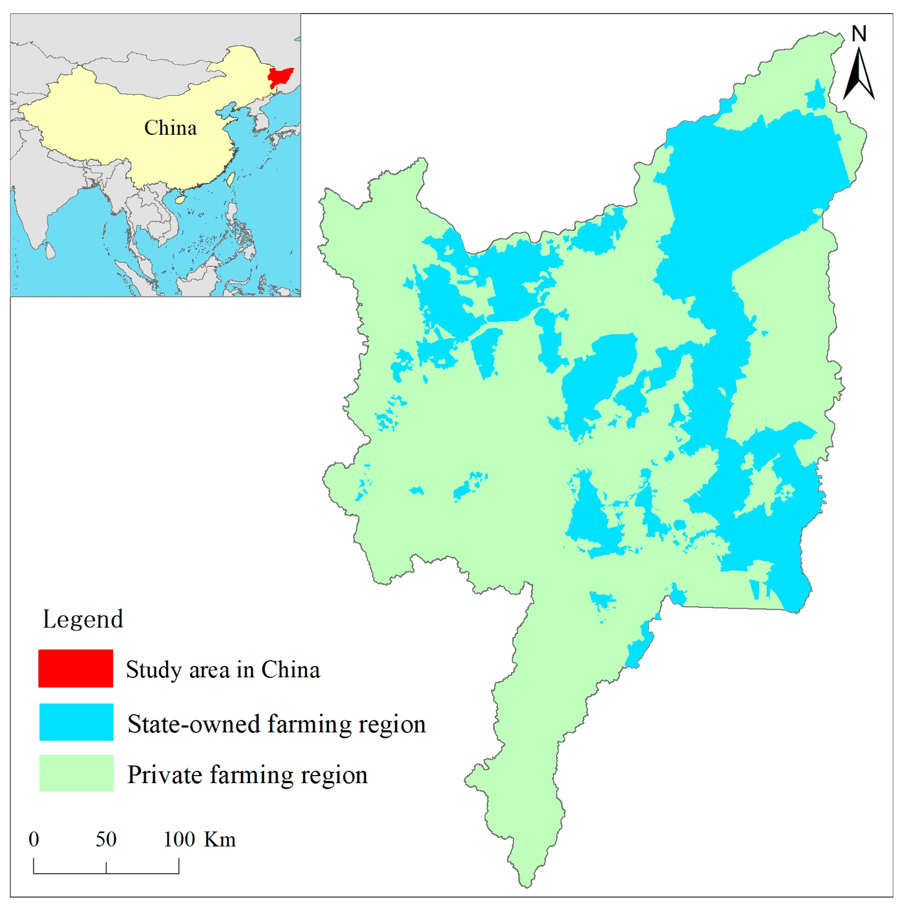
2.1. Study Area

Sanjiang Plain is located in the northeast region of China (Figure 1), with latitudes of 43°–48° N and longitudes of 129°–135° E. The terrain of this region is mainly plain with an average altitude of 60 m. It has a continental monsoon climate. The lowest temperature occurs in January and highest temperature occurs in July. The natural vegetation of Sanjiang Plain is dominated by marshy meadows. The wet and marsh plants mainly include a small leaf chapter, marsh willow, moss grass, and reeds. Among them, the moss grass marsh is the most widely distributed, accounting for about 85% of the total area of the marsh, followed by the reed marsh. The soil types of Sanjiang Plain are mainly black soil, white pulp soil, meadow soil, marsh soil, etc., and meadow soil and marsh soil are the most widely distributed. The color of the land surface is mainly covered by black soil with high organic matter content. Sanjiang Plain has sufficient water resources, and the main rivers include Heilongjiang River, Wusuli River, and Songhua River. Natural conditions such as flat terrain, unique black soil, and abundant water resources make it suitable for agricultural development. At the same time, land management systems of Sanjiang Plain (Figure 1) include state-owned farms (i.e., the total land area of 3.42 × 10⁴ km2) and private farms (i.e., the total land area of 7.45 × 10⁴ km2) [47]. The Sanjiang Plain is also a typical area of China’s commodity grain production base and land management system, acting as the pioneers in the reform of China’s arable land-planting structure and land management system. Therefore, the government departments at different levels (i.e., central and local governments) have been implementing a variety of agricultural policies and water conservancy engineering in this region to support food security and the development of high-quality rice/corn. This region has also become one of the hotspots in land research in China.

2.2. Research Data and Methods

2.2.1. Data Collection and Processing

In this section, all the basic data required in this study mainly include three parts, including land-use data, statistical data, and other data. For the obtaining of land-use data, the time of land data in 1990, 2000, 2010, and 2015 were obtained from the data platform of the Institute of Geographic Sciences and Resources, Chinese Academy of Sciences (website: https://www.resdc.cn/, accessed on 13 July 2022), wherein the format of land data was a vector, which can effectively improve the calculation accuracy comparing with a raster format. To check the accuracy of land-use data in the study area, Landsat TM/ETM+/OLI satellite images (Table 1) in 1990, 2000 2010, 2015, and 2020 were downloaded from the United States Geological Survey, USGS (website: http://glovis.usgs.gov/ on 13 July 2022). These images were synthesized with false color synthesis method on the ENVI platform. Then, human–computer interactive visual interpretation inspection for each period of images was applied using professional geoscience knowledge, such as the spot size, color, and texture characteristics, of land types from remote-sensing images, to correct potentially inaccurate land-use patches. After that, we overlapped the 2015 vector land-use data onto the 2020 Landsat image to obtain the 2020 land-use data of Sanjiang Plain through the method of manual digitization on the ArcGIS 10.8 software platform Finally, the method of stratified random sampling was applied for the first-level land type validation in 1990, 2000, 2010, and 2020 using the remote-sensing satellite imagery (i.e., Landsat images and high-resolution Google satellite).
For the land-use classification system, the land data used in this study contained six first-land class types, including cultivated land, forest land, grassland, waters, construction land, and unused lands. On the basis of six first-land class types, the land-use classification system was further divided into 25 s-land class types, including paddy fields, upland crops, woodland, shrub wood, sparse woods, other forest land, high and medium density grassland, low density grassland, rivers, lakes, reservoirs, ponds, tidal flats and beaches, permanent glacier and snow, urban land, rural land, industrial and mining land, bare rock land sandy land, wetland, bare land, gobi, saline alkali land, etc.
For statistical data, it was mainly from the statistical yearbook of Heilongjiang Province (i.e., a provincial-level administrative unit in China covering the entire Sanjiang Plain) and its subordinate cities and counties, state-owned farms, local archival materials, etc. Main statistical indicators include the main crop sowing area, the main crop yield, grain net profit, etc.
Other relevant data include administrative division data and the boundary of different land management system regions, which were obtained from the academic research institution, namely the Institute of Geographic Sciences and Natural Resources, Chinese Academy of Sciences.

2.2.2. Land-Use Dynamics Tracking Techniques and Dynamic Degree

(1) Land dynamic tracking technique is a better method for studying the trajectory of land-use change in multiple time periods (Figure 2). This method cannot only track the changing process of all types of land use, but it can also track the source and destination of a certain land component or the differential change, thereby revealing the mechanism of land time and space change trajectory [47,49].
(2) Dynamic degree of land use is a quantitative measure of the degree of change in the quantity of a certain type of land use within a certain time range or in multiple time periods, in which large values indicate drastic changes and small values indicate relatively slow changes. The core formula is as follows:
K = S j S i S i × 1 T × 100 %
where K represents the rate of change, S i and S j are the areas, and T is the whole research period.

2.2.3. Landscape Pattern Analysis

Landscape index highly concentrates the information of land-use landscape in the process of the different land-use change. It can display the composition, spatial distribution, and changes in different landscape structure, which is a quantitatively reliable method and is widely applied in academic surveys [50]. Due to the large correlation among multiple landscape indexes, more indexes may be redundant and fewer indexes cannot express all information. Therefore, landscape index screening is needed to express all research content using the least number of landscape indexes. In this study, we select as few landscape indexes as possible to comprehensively express landscape objectives, including the research objectives of landscape comprehensive changes, the dominance, the aggregation, the degree of edge variation in landscape type, and the degree of adjacency of the different landscape types. The survey objectives of these five perspectives can generally express the evolution process of land landscape. To find the universal landscape index that matches these research objectives, we searched for academic literature [51,52], and used the user guide document of landscape. Finally, the Shannon’s Diversity Index, Largest Patch Index, Aggregation Index, Landscape Shape Index, and Interspersion and Juxtaposition Index are selected, wherein Shannon’s Diversity Index reflects the comprehensive regularity of different patches or landscapes (i.e., fragmentation or integrity). The Largest Patch Index refers to the percentage of the largest patch in the total area, reflecting the degree of advantage in landscape change. The Aggregation Index reflects the degree of interconnection between patches of the same type. The Landscape Shape Index reflects the shape dispersion and regularity of edge landscape shape variation. The Interspersion and Juxtaposition Index reflects the distribution and parallel distribution of different landscape types and shows the interaction between different types. These indexes were calculated in the landscape metrics model and class metrics model on Fragstats4.2 Software Platform (Table 2), respectively.

2.2.4. The Valuation of the Ecosystem Services

Methodology of the ecosystem service equivalent factor evaluation model proposed from Xie Gaodi has been widely used in academic research [31,32,53,54,55,56]. Core elements of this evaluation model include an ecological classification system, an equal factor table, and the factor value. After statistical analysis, these statistical results are linked to the land-use attribute table, forming a spatialized map of ecosystem service values.
For the first core element (i.e., an ecological classification system), Xie Gaodi’s research provides a classification of ecosystems. In this study, we use the land-use data of the Chinese Academy of Sciences due to the better accuracy and richer land classifications. We compare the meanings of different land types in these two land classification systems. After one-to-one correspondence between the land types of two classification systems, Table 3 is obtained.
In Table 3, we make some improvements in construction land. In Xie’s research, Construction land is set as a desert system. This setting may imply an underestimation of ecosystem services for construction land (i.e., urban, rural, and industrial). Starting from this point, we mainly use high-resolution satellites to classify construction land to obtain the sub-construction land types. We fully consider the actual situation of construction land in Sanjiang Plain and divide the construction land into different sub-types such as buildings, forests, and grasslands. After that, these land-use categories are merged into different ecosystems, such as forest ecosystems, grassland ecosystems, desert ecosystems, etc. Then, the ecosystem service measurement of construction land was close to the real surface cover values.
The next question is how to classify and verify construction land. Before this, the first step is to reasonably determine the internal land classification system for construction land. As we all know, there are various land types within the construction land, including buildings, roads, squares, lawns, green trees on both sides of roads, park vegetation areas, as well as bare soil. The surface area of buildings, roads, and squares without vegetation coverage can be regarded as impervious surface area. The lawns, green trees on both sides of roads, and parks are merged into forest land and grassland. Bare soil can be regarded as bare land. Therefore, the construction land in Sanjiang Plain was divided into a total number of four types of land covers, covering impervious surface area, forest land, grassland, and bare soil.
After that, the internal classification of construction land is implemented. To accurately classify construction land, high resolution satellite images accompanied by a resolution of 0.5 m on professional and paid platforms (website: https://www.91weitu.com/ on 13 July 2022) are downloaded, and the automatic classification technology is used on the Envi platform. Then, we obtain the land-use maps within the construction land. To ensure classification quality, human computer interaction visual inspection is applied to correct incorrect land patches. After that, layered random sampling method is used for accuracy evaluation, and we obtain a comprehensive accuracy of over 96% for land classification within the construction land.
The next question is to calculate the proportion of different land types (i.e., impervious surface area, forest land, grassland, and bare soil) within the construction land. The proportion of impervious surface area, forest land, grassland, and bare soil within the construction land of Sanjiang Plain are 62.59%, 16.67%, 16.67%, and 3.05%, respectively, i.e., 4/6 impervious surface and bare soil, 1/6 forest land, and 1/6 grassland. These data are added to Table 3. The matching of the ecosystem is completed.
For the second core element (i.e., an equal factor table), the factor table of different ecosystems from Xie’s study are determined through actual observations and experiments. This means it has good accuracy. In the study, according to Table 3, we calculate and obtain Table 4. In the calculation process of Table 4, it can be understood that the factor of paddy fields from Xie’s study can be directly given the paddy fields in this study, due to the land types being the same. Also, the factor of river system from Xie’s study is given to the land types of reservoirs, ponds, tidal flats, beaches, rivers, and lakes, due to the land classification system of this study having more water classification types. By calculating each factor in this way, we obtain all the factors in Table 4. For Table 4, ecosystem services are divided into the functions of supply, regulation, support, and culture. For supply function, it mainly provides food production (FP), raw material production (MP), and water resources supply (WRS). Regulation function includes gas regulation (GR), climate regulation (CR), purification environment (PE), and hydrological regulation (HR). Support function contains soil conservation (SC), maintaining nutrient cycle (MNC), and biodiversity (BD). Culture function mainly refers to the aesthetic landscape (AL). These four functions constitute the main structure of ecosystem services and affect many elements of human production, life, and ecological environments.
The third core issue is calculating the monetary value of different ecosystem service functions. On the basis of Table 3 and Table 4, we should obtain the factor value (i.e., the monetary value of a factor equivalent). From Xie’s study, Equation (2) is used to calculate this. To ensure the accuracy of the data, all data come from statistical yearbooks and the archived materials in this calculation process. After that, the cultural services, support services, supply services, and regulation services, as well as the sub-level ecosystem service value, are calculated (i.e., Table 5). Finally, the total value of ecosystem services is calculated using Equation (3):
E a = 1 7 i = 1 n m i p i q i M
where, E a is the economic value of the food production service function provided by the farmland ecosystem per unit area (yuan/ha), M is the planting area of all crops (ha), p i is the national average price of i crop in a year (yuan/ton), m i is the planting area of i crop (ha), q i is the yield per unit area of i crop (ton/ha), and i is the crop type.
E S V = A i × V C i
where ESV is the total value amount of ecosystem service, V C i is the value coefficient of the i land class, and A i is the area of the i land class.
Furthermore, spatial distribution maps of ecosystem service values intuitively reveal and compare the spatiotemporal distribution differences in ecosystem service values in different land management system regions (i.e., state-owned farms and private farms). A spatial distribution map of ecosystem service needs to be produced. Through from Section 2.2.1, Section 2.2.2 and Section 2.2.3, we understand that the vector land-use maps come from Landsat images. Its first-land classification system contains cultivated land, forest land, grassland, waters, construction land, and unused lands. For the construction land, we classify its internal structure to subclass types (i.e., impervious surface area, forest land, grassland, and bare soil) using 0.5 m high resolution satellite imagery. Then, the data format of subclass type map is converted from raster to vector using spatial analysis tools. The converted vector map is further used to erase the construction land from the vector land-use map of the study area to obtain the land-use map that does not contain the construction land. The vector subclass type map within the construction land and the vector land use without construction land are merged for a new map. Then, the spatial map of ecosystem service is presented on state-owned farms and private farms through overlaying administrative division data. After that, this study classifies the calculated ecosystem service value results into five levels, including the ecosystem service low-value area (i.e., level I), ecosystem service sub-low value area (i.e., level II), ecosystem service median-value area (i.e., level III), ecosystem service sub-high value area (i.e., level IV), and ecosystem service high-value area (i.e., level V), respectively.

3. Results

3.1. Land Data Accuracy Evaluation

The method of stratified random sampling is applied for the first-level land type validation in 1990, 2000, 2010, and 2020 in this study, and the classification results are displayed in Table 6. Overall, land accuracies are 91.83%, 93.17%, 95.51%, and 95.33% in 1990, 2000, 2010, and 2020, with corresponding kappa coefficients of 0.88, 0.88, 0.88, and 0.89, respectively. Data display that the latter years (i.e., 2010 and 2020) have the higher overall accuracy than the former years (i.e., 1990 and 2000), due to the improved Landsat image intensity and the availability of high-quality Google Earth imagery during the land validation process. Meanwhile, for the accuracy in different land-use types, the construction land always shows better user’s accuracy (UA) in each year, specifically UA (96.88%) in 1990, UA (96.77%) in 2000, UA (96.97%) in 2010, and UA (100.00%) in 2020. This can be attributed to the fact that construction land, such as urban and rural areas, is more easily recognized through human–computer interaction. In addition, the classification error samples of water land, cultivated land, and unused land can be attributed to the paddy fields in cultivated land and the swamp wetlands in unused land. There are also low error samples between forest land and grassland. Overall, the time series maps of land use in Sanjiang Plain display high accuracies and can be used for land change and its environmental survey in this study.

3.2. Spatiotemporal Characteristics of Current Land Status and Dynamic Change Trend in Different Land Management System Regions from 1990 to 2020

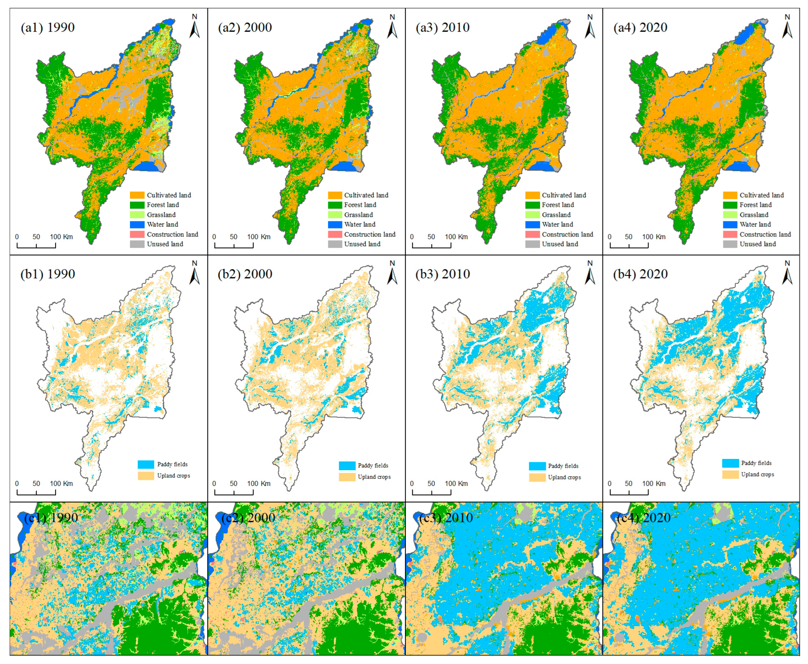
3.2.1. Analysis of the Spatiotemporal Variations in Land Use in the Whole Sanjiang Plain from 1990 to 2020

Geographical maps of land distribution in 1990, 2000, 2010, and 2020 were obtained (Figure 3) using the land-use vector data. In 1990, the area of cultivated land, forest land, grassland, water area, construction land, and unused land were 46,194.48 km2, 35,971.64 km2, 8103.39 km2, 5509.27 km2, 2121.69 km2, and 10,752.37 km2, accounting for 42.52%, 33.11%, 7.46%, 5.07%, 1.95%, and 9.90%, respectively. And, in 2020, the corresponding area of these land types were 58,642.04 km2, 32,663.02 km2, 2072.52 km2, 5033.46 km2, 2524.95 km2, and 7715.10 km2, accounting for 53.97%, 30.06%, 1.91%, 4.63%, 2.32%, and 7.10%, respectively. Data displayed that the corresponding area changes in cultivated land, forest land, grassland, water area, construction land, and unused land were 12,447.56 km2, −3308.62 km2, −6030.86 km2, −475.81 km2, 403.25 km2, and −3037.27 km2 from 1990 to 2020, with increments of 11.36% and 0.37% in cultivated and construction lands, and the decreases of −3.04%, −5.55%, −0.44%, and −2.80% in forest land, grassland, water area, and unused land. Therefore, land-use change in the whole study area was mainly driven by violent cultivated land expansion.
Cultivated land displayed the highest increment in Sanjiang Plain, with a net increase of 12,447.56 km2 from 1990 to 2020, wherein the change area of cultivated land was 7008.10 km2, 5074.44 km2, and 365.01 km2 in the periods of 1990–2000, 2000–2010, and 2010–2020, illustrating that the trend of cultivated land expansion continued to decrease in each period. In the context of intense expansion of cultivated land, the continuous differential changes in cropping structure were also monitored, such that the areas of upland crops were 39,241.36 km2, 44,878.72 km2, 37,297.74 km2, and 31,980.51 km2 in 1990, 2000, 2010, and 2020, with a loss of 7260.85 km2 and a decrease rate of 6.68% from 1990 to 2020. In three stages, the changes in the area of upland crops were +5637.36 km2, −7580.98 km2, and −5317.22 km2, showing an increasing trend first followed by a decreasing trend. On the contrary, the areas of paddy fields were 6953.12 km2, 8323.86 km2, 20,979.28 km2, and 26,661.52 km2 in 1990, 2000, 2010, and 2020, with an increment of 19,708.40 km2 and an increased rate of 18.14% from 1990 to 2020, accompanied by corresponding increments of 1370.74 km2, 12,655.43 km2, and 5682.24 km2 for each time period. Data showed that paddy fields displayed a drastic increase during the studied period.
A Sankey diagram of Sanjiang Plain from 1990 to 2020 is displayed in the Figure 4. From this figure, the land conversion process of figure a, b, and c is different, indicating the differentiated land changes in the periods of 1990–2000, 2000–2010, and 2010–2020, respectively. Statistical data based on land conversion displayed that from 1990 to 2000, the biggest land conversion process is from upland crops to paddy fields, with a total area of 3299.89 km2, followed by the main land conversion of paddy fields to upland crops, grassland to upland crops, forest land to upland crops, and unused land to upland crops, with corresponding areas of 2667.45 km2, 2614.57 km2, 1927.90 km2, and 1911.97 km2, respectively. Compared to 1990–2000, 2000–2010 had the biggest land conversion process changes from upland crops to paddy fields, with a bigger area of 9633.86 km2, followed by the main land conversion of forest land to upland crops, unused land to upland crops, upland crops to forest land, water land to unused land, and unused land to paddy fields. Similarly, for 2010–2020, the biggest land conversion process was still from upland crops to paddy fields, with a total area of 5361.06 km2. However, the conversion area of other lands was very small in 2010–2020, and the biggest was from grassland to paddy fields, with only an area of 184.37 km2.

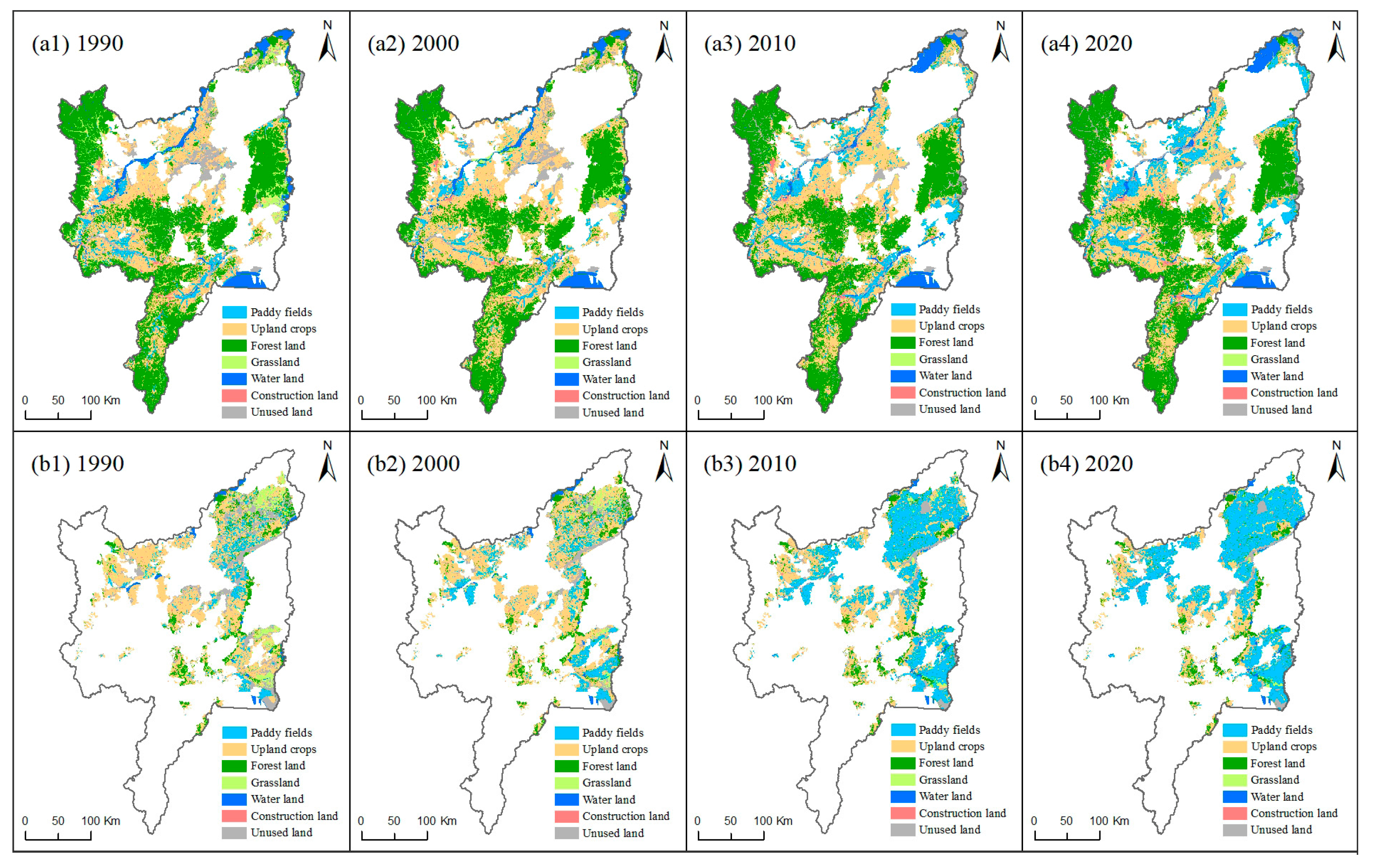
3.2.2. Comparative Analysis of Land Spatiotemporal Characteristic Changes in Different Land Management System Regions from 1990 to 2020

For different land-use types, a comparative analysis of different land changes on state-owned farms and private farms was revealed. On state-owned farms (Figure 5), the forest land, grassland, water area, and unused land showed a decreasing trend with changes of −924.63 km2, −2338.63 km2, −185.94 km2, and −2796.08 km2 from 1990 to 2020. Data indicated that the reduction in grassland and unused land was more drastic. In contrast, cultivated and construction lands exhibited an ascending feature, with a change of 6156.70 km2 and 87.24 km2, respectively. For changes in land rate, the rate of forest land, grassland, water area, and unused land reduced from 11.91%, 9.32%, 2.74%, and 16.60% in 1990 to 9.21%, 2.47%, 2.20%, and 8.42% in 2020, with changes of −2.71%, −6.84%, −0.54%, and −8.18%, respectively. On the contrary, the rate of cultivated and construction lands increased from 58.25% and 1.17% in 1990 to 76.27% and 1.42% in 2020, with a large increment of 18.02% in the former and only a small increment of 0.26% in the latter, respectively. Therefore, the increment of cultivated land was large, and its proportion in 2020 has exceeded three quarters on state-owned farms. While on private farms, a similar changing law was that forest land, grassland, water area, and unused land exhibited a descending feature; on the contrary, the cultivated and construction lands exhibited an ascending feature, comparing to state-owned farms. But, the obvious difference was that the loss of forest land, grassland, and water area were more drastic on private farms, with a loss of −2383.99 km2, −3692.24 km2, and −289.87 km2 from 1990 to 2020, which was 2.58 times, 1.58 times, and 1.56 times the land types of state-owned farms. However, the loss of unused land was very small on private farms, only 0.09 times that of state-owned farms. By monitoring, we found that these lost lands were mainly transferred to cultivated land on state-owned farms and private farms. Differently, a large amount of loss in forest, grassland and waters on private farms were mainly changed into cultivated land, which promoted its increase by 6290.86 km2. But, on state-owned farms, the source of cultivated land expansion was largely from unused land, accompanied by an increment of 6156.70 km2.
A comparative analysis from the perspective of different internal structure changes in cultivated land was then revealed. Although the increasement in cultivated land on state and private farms were nearly equivalent (6156.70 km2 vs. 6290.86 km2) from 1990 to 2020, there were obviously different trends in the internal structure of cultivated land (i.e., upland crops and paddy fields). On state-owned farms, paddy fields exhibited a drastic growth feature, with the area changing from 3466.48 km2 in 1990 to 17,254.81 km2 in 2020, a change of 13,788.32 km2, and with a change of 1899.79 km2, 9085.07 km2, and 2803.46 km2 in 1990–2000, 2000–2010, and 2010–2020. This indicated that paddy fields showed a continuous increase feature. In contrast, upland crops exhibited a falling feature, with the area decreasing from 16,436.09 km2 to 8804.47 km2, a net change of −7631.62 km2, and with changes of 1164.12 km2, −6266.20 km2, and −2529.54 km2 in each period, exhibiting the change characteristic of first increasing and then decreasing. While on private farms, although paddy fields increased from 3486.63 km2 in 1990 to 9406.72 km2 in 2020, only a change of 5920.08 km2, the change was much smaller than that of state-owned farms (i.e., 5920.08 km2 vs. 13,788.32 km2). Changes in paddy fields during different periods were −529.05 km2, 3570.36 km2, and 2878.77 km2, exhibiting the feature of first decreasing and then increasing, which was also different from the continuous increase characteristic of paddy fields on state-owned farms. Meanwhile, upland crops increased from 23,176.04 km2 to 22,805.27 km2, with a net change of 370.78 km2 from 1990 to 2020, while upland crops on state-owned farms showed a large decrease. Therefore, cultivated land expansion on state-owned farms showed an increase in paddy fields but a decrease in upland crops, while those on private farms exhibited an increase in both land types of paddy fields and upland crops.

3.3. Landscape Analysis from Different Scales in Different Land Management System Regions from 1990 to 2020

Comparative analysis at landscape scale was first executed. Landscape diversity in Sanjiang Plain was basically constant from 1990 to 2020, at around 1.56. However, we found the opposite trend of landscape diversity in different land management system regions. Among which (Figure 6), landscape types became richer on private farms (SHDI = +0.63%), but it was a decrease in landscape richness and an increase in integrity on state-owned farms (SHDI = −9.88%). Meanwhile, on state-owned farms, land-use pattern dominated by continuous rapid expansion of paddy fields promoted the increasing degree of landscape aggregation (AI = +0.43%) and increased the spatial sprawl among the different land-use types (IJI = +4.27%), which also brought the tendency of landscape shape to be simplified (LSI = −13.30%). While on private farms, the continuous encroachment of cultivated land (i.e., paddy fields and upland crops) to other surrounding lands resulted in a decrease in the degree of ecological landscape integrative aggregation (AI = −0.56%). This further caused more complex shapes among patches (LSI = +23.3%) and increased proximity among different land types (IJI = −4.28%).
Comparative analysis at the land-use type scale was then executed (Table 7). In this section, we compared the landscape types and summarized their change regularity in different land management system regions. On state-owned farms, the reduction in the area of upland crops, forest, grassland, waters, and unused land brought about the decrease in LPI, with values of −3.58, −0.14, −2.07, −0.32, and −1.21 from 1990 to 2020, and the decrease in AI, with corresponding changes of −0.65, −0.67, −2.43, −2.37, and −0.85, respectively. In contrast, the expanded area of paddy fields and construction land promoted the enhancement in LPI and the degree of AI by 21.01, 0.02, and 3.11, 0.45, respectively. Among these values, the greatest variation was observed in paddy fields, especially in LPI, with increments up to 21.02. At the same time, the LSI of paddy fields, grassland, upland crops, and unused land became simplified, but forest, waters, and construction land were more complex. According to the survey, the changes in LSI of forest land change were mainly concentrated in a farming–pastoral ecotone, and the expansion of construction land brought about its landscape shape complexity mainly in urban regions.
On private farms, the different landscape changes were monitored compared to the state-owned farms. The changes in the LPI of paddy fields, upland crops, forest land, grassland, water area, construction land, and unused land were 0.59, 0.39, −0.40, −0.47, −0.07, 0.06, and −1.95, accompanied by the corresponding AI values of 0.95, −0.84, −0.55, −4.36, −0.51, 0.49, and −1.87, respectively. Data indicated that the changes in LPI and AI were much smaller on private than that of state-owned farms. Meanwhile, the changes in LSI among land types of paddy fields, upland crops, forest, grassland, waters, construction, and unused lands were 8.82, 43.37, 28.06, −6.70, 10.06, 0.29, and 41.94. This means that the LSI in all land types become more complex, except for grassland on private farms, and only the LSI of forest, waters, and construction land became more complex on state-owned farms. We also found that the paddy fields with the largest change had a simple LSI on private farms, while in contrast, it was more complex on state-owned farms. Our survey found that paddy fields were well-planned by the agricultural management department, forming a concentrated and contiguous planting pattern on state-owned farms. While on private farms, farmers themselves planted paddy fields, for which the degree of concentration was low; paddy fields may have been surrounded by other land-use types, which promoted the complexity in LSI.

3.4. Analysis of Spatiotemporal Characteristics of Ecosystem Service Values between the Different Land Management System Regions from 1990 to 2020

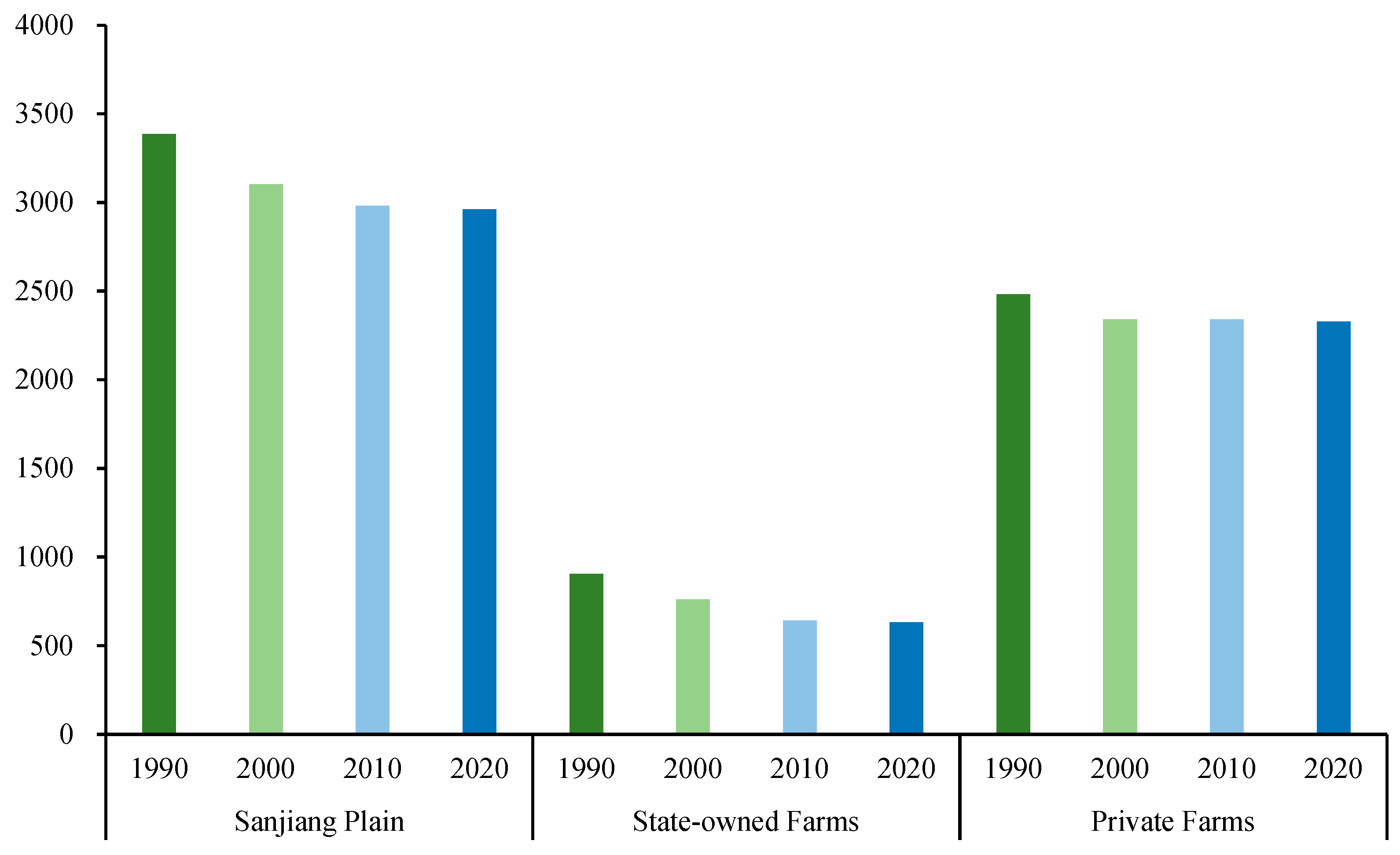
3.4.1. Comparison Analysis of the Differentiated Ecosystem Service Changes under Different Land Management System Regions

This study improved the ecosystem service measurement method and evaluated its value in Sanjiang Plain (Figure 7). Total ecosystem service value was 338.62, 310.16, 298.17, and 296.03 × 10⁹ yuan in 1990, 2000, 2010, and 2020, with a net decrease of 42.60 × 10⁹ yuan and a loss rate of 12.58% from 1990 to 2020, indicating a serious loss of ecosystem services. We also monitored that its change was different in each period, namely a loss of −28.46 × 10⁹ yuan, −11.99 billion yuan, and −2.15 billion yuan in 1990–2000, 2000–2010, and 2010–2020, respectively, which indicated that the loss of ecosystem services in Sanjiang Plain was slowed down.
Different ecosystem service changes were monitored in different land management system regions. Firstly, in terms of total quantity, on private farms, the total amount of ecosystem services decreased continuously from 248.19 × 10⁹ yuan in 1990 to 232.86 × 10⁹ yuan in 2020, with a loss of 15.33 × 10⁹ yuan. The corresponding loss rate was only 6.18%, which was much lower than the average level of the whole study area. However, on state-owned farms, the total amount of ecosystem services decreased continuously from 90.43 × 10⁹ yuan in 1990 to 63.16 × 10⁹ yuan in 2020, with a loss of 27.27 × 10⁹ yuan. The corresponding loss rate was as high as 30.15%, which was much higher than the average level of the whole study area. Data indicated that the loss rate of state-owned farms was 4.88 times than that of private farms. Secondly, in terms of the characteristics at different periods, on private farms, the loss of ecosystem service was −14.11 × 10⁹ yuan, −0.08 × 10⁹ yuan, and −11.37 × 10⁹ yuan in the three periods of 1990–2000, 2000–2010, and 2010–2020, respectively, showing a W-shaped loss characteristic. However, on state-owned farms, the loss in the three periods was −14.35 × 10⁹ yuan, −11.91 × 10⁹ yuan, and −1.01 × 10⁹ yuan, which showed a continuous downward trend.

3.4.2. Comparison Analysis of Spatial Ecosystem Service Evolution in Different Land Management System Regions

According to the spatial classification patterns of ecosystem service values in Sanjiang Plain in 1990, 2000, 2010, and 2020 (Figure 8 and Figure 9), we found that ecosystem service values of the whole region exhibited high areas were concentrated in the eastern, western, and southern regions, while low areas were concentrated in the central and northern regions. In different land management system regions, there were obviously spatial distribution differences. On state-owned farms, the space distribution of category I had rapidly expanded; by contrast, the space distribution of category II, III, IV, and V were obviously reduced in size from 1990 to 2020. Compared to state-owned farms, the expansion of category I was slow on private farms, along with the relatively slow expansion of other categories. Finally, in 2020, the category I was widely distributed on state-owned farms, but on private farms, both category I and category V presented spatially extensive distribution, among which category V was mostly located in the edge.

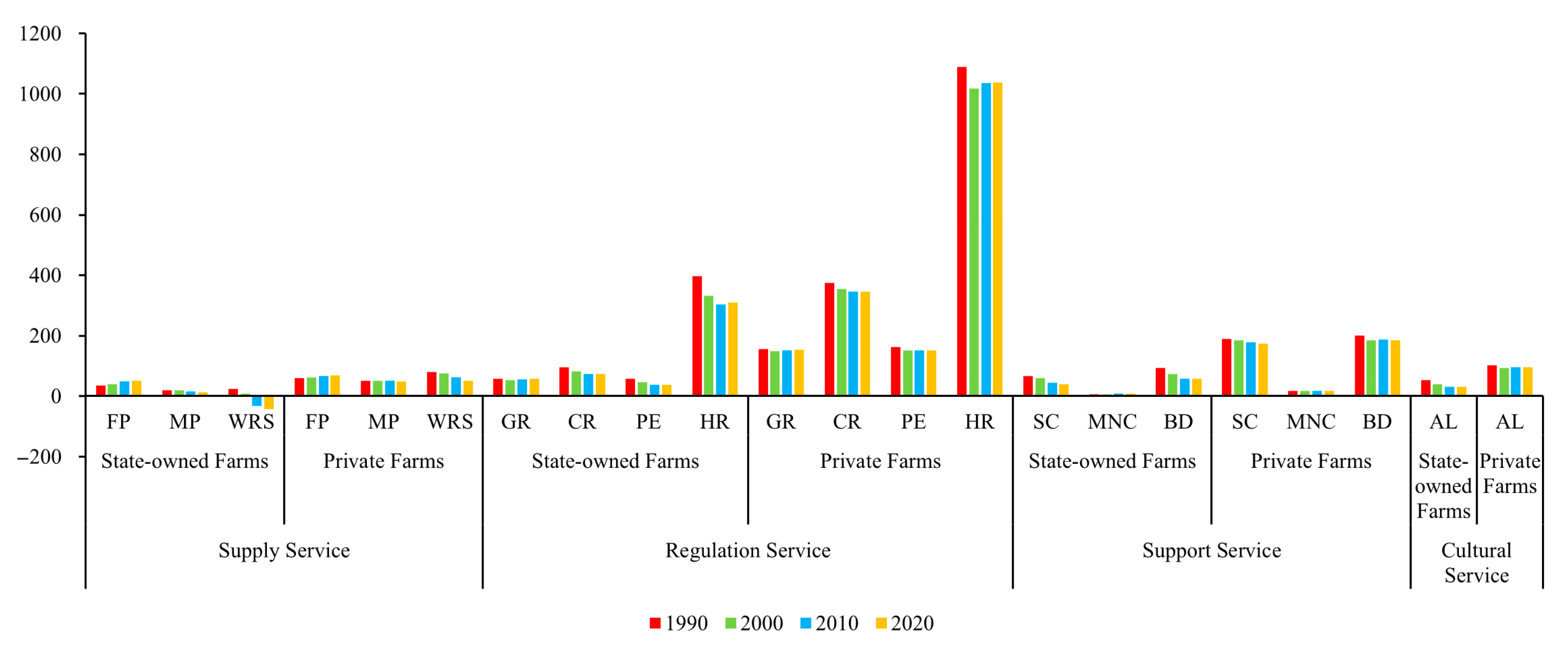
3.4.3. Comparative Analysis of Different Ecosystem Service Functions on State and Private Farms

According to the calculation results of ecosystem service (Figure 10), the differences in state and private farms were comparatively analyzed from four aspects, including the services functions of supply, regulation, support, and culture. Firstly, for supply service function, only the value of food production continued to increase, with an increase of 1.46 × 10⁹ yuan on state-owned farms and 0.98 × 10⁹ yuan on private farms. Others showed a continuous declining trend, such as water resources decreasing by 6.70 × 10⁹ yuan on stated-owned farms and 2.91 × 10⁹ yuan on private farms. Secondly, for regulation service, the proportion of climate and hydrological regulation functions were high, and the sum of these two reached over 80% in both regions, but a downward trend was monitored, with −2.38 × 10⁹ yuan and −2.92 × 10⁹ yuan on state-owned farms and −2.92 × 10⁹ yuan and −5.18 × 10⁹ yuan on private farms, respectively. Thirdly, for support service, the contributions of soil conservation and biodiversity were obvious, with both showing a continuous decreasing trend, with the changing values of −2.81 × 10⁹ yuan and −3.66 × 10⁹ yuan on state-owned farms, and −1.49 × 10⁹ yuan and −1.47 × 10⁹ yuan on private farms, respectively. Maintaining nutrient cycling function continued to increase by 0.12 × 10⁹ yuan in the former, but it decreased first and then increased in the latter, with a net change of 0.0057 × 10⁹ yuan. Fourthly, for cultural service, the aesthetic landscapes continued to decrease in both regions from 1990 to 2020, with reductions of 2.16 × 10⁹ yuan on state-owned farms and 0.73 × 10⁹ yuan on private farms.

3.4.4. Comparative Analysis of Ecological Service Functions from Different Land Types on State and Private Farms

On the whole, the number of high-value land types (i.e., forest, grassland, waters, and wetland) is decreased; on the contrary, the contribution of cultivated and construction lands with low ecological value increased, resulting in a total loss in the study area from 1990 to 2020. On state-owned farms, the total amount of ecological services divided by land type follows wetland > water area > forest > cultivated land, with a rate of 47.71%, 19.05% 12.91%, and 12.84% in 1990. In 2020, the order was wetland > cultivated land > water area > forest, with a rate of 34.60%, 21.85%, 15.22%, and 23.71%. Data showed that the order of cultivated land was moved forward. Differently, on private farms, the total amount of ecological services divided by land type follows forest > waters > wetland > cultivated land, with rate of 38.94%, 33.83%, 15.53%, and 6.19% in 1990. And, in 2020, the order was not changed, only with the corresponding rates of 38.88%, 33.75%, 15.75%, and 8.13%, respectively.
Furthermore, on state-owned farms, the ecosystem service value of wetland reduced from 43.15 × 10⁹ yuan in 1990 to 21.86 × 10⁹ yuan in 2020, with a decrease of 21.29 × 10⁹ yuan (Figure 11). This showed that wetland was the land type losing the most value in ecosystem services, followed by grassland, a loss of 4.12 × 10⁹ yuan. In different types of grassland, the service value of high and medium coverage grassland lost more, compared to the low-coverage grassland. Net decrease in forest ecosystem services was 2.06 × 10⁹ yuan, of which the loss of shrub forest, sparse forest, and other woodland was 1.81 × 10⁹ yuan, 1.24 × 10⁹ yuan, and 0.03 × 10⁹ yuan, respectively, while woodland increased by 1.03 × 10⁹ yuan. In contrast to these ecosystem service reductions, ecosystem services of cultivated and construction lands increased by 3.37 × 10⁹ yuan and 0.25 × 10⁹ yuan, respectively. For the internal structure of cultivated land, paddy fields increased by 7.84 × 10⁹ yuan, while upland crops decreased by 4.48 × 10⁹ yuan from 1990 to 2020.
On private farms, the loss of ecosystem services in forest, grassland, and water area were relatively large, with values of 6.11 × 10⁹ yuan, 6.51 × 10⁹ yuan, and 5.36 × 10⁹ yuan, respectively. Then, followed by wetland, values of −5.46 × 10⁹ yuan, +4.47 × 10⁹ yuan, and −8.4 × 10⁹ yuan in 1990–2000, 2000–2010, and 2010–2020, respectively, were observed, showing a decreasing trend in fluctuations. By contrast, cultivated land and construction land had a positive effect on ecosystem service, with increments of 3.59 × 10⁹ yuan and 0.92 × 10⁹ yuan. For the internal structure of cultivated land, the increment of paddy fields and upland crops were 3.37 × 10⁹ yuan and 0.22 × 10⁹ yuan, respectively. Further, the total increase in the ecosystem service of cultivated and construction lands was greater on private than that of state farms.

4. Discussions

4.1. Cultivated Land Continues to Increase in Sanjiang Plain, and Is Accompanied by a More Differentiated Pattern of Upland Crops and Paddy Fields in Different Land Management Systems in Northeast China

According to the previous literature [26,57], the evolution of cultivated land has undergone different spatial migration patterns in China. Initially, primitive cultivated land was largely located in Southeast China due to suitable temperature and climate. This region has also been awarded the title of “Jiangnan fish and rice region of China”. With urban–rural expansion, and the increase in industrial and mining lands, lots of high-quality cultivated land featured by double-cropping in each year or triple-cropping in two years in the southeast region was invaded and lost. Under the background of cultivated land loss and population growth, cultivated land reclamation shifted from Southeast China to Northeast China, and then, Northeast China became a new expansion hotspot area for cultivated land [6]. In the past half century, lots of cultivated lands have been reclaimed in the northeast region, which become the granary of China, especially in Sanjiang Plain. Afterwards, cultivated land reclamation shifted from Northeast China to Northwest China such as Xinjiang, due to the suitable cultivated land resources in Northeast China that were basically exploited [6]. From 1990 to 2015, China’s cultivated land resources experienced a trend characterized by an increase (1990–2000) and then a gradual decrease (2000–2015) [47,58]. So, against the backdrop of continuous decline in cultivated land resources nationwide [46], this study monitored that the cultivated land in Sanjiang Plain in 1990, 2000, 2010, and 2020 was 46,194.48 km2, 53,202.58 km2, 58,277.02 km2, and 58,642.04 km2, with a total increase of 12,447.56 km2, indicating a continuous increasing trend. We also monitored that the changing area of cultivated land in 1990–2000, 2000–2010, and 2010–2020 were 7008.10 km2, 5074.44 km2, and 365.01 km2, respectively, indicating that the growth trend of cultivated land slowed down in each period.
Influenced by different land management systems, the land changes in state-owned farms and private farms were also different, especially for paddy fields and upland crops. On state-owned farms, from 1990 to 2020, the area of paddy fields increased from 3466.48 km2 to 17,254.81 km2, while upland fields decreased from 16,436.09 km2 to 8804.47 km2, showing a violent increase in paddy fields and an acute decrease in upland crops. On private farms, the covered area of paddy fields increased from 3486.63 km2 to 9406.72 km2, and upland crops changed from 22,805.27 km2 to 23,176.04 km2, showing an increase in both paddy fields and upland crops. The land management system and farming mode acted as the significant functions during this process. The reclamation area with state land ownership has a faster process of paddy conversion than the agricultural area with collective land ownership. In addition, the transformation of the large scale of upland crops to paddy fields in Sanjiang Plain occurred mainly in state-owned farms. On the one hand, due to the fact that the land in the reclamation area belongs to the state, a large number of agricultural policies and water conservancy projects were implemented in state-owned farms [46,47], which can meet the basic conditions for continuous and large-scale planting of paddy fields. On the other hand, because the behavior of the farm household was affected by the price of agricultural products, the willingness of farmers to change to rice planting increased, due to the increase in the expected minimum purchase price level for rice. Also, the different median size of the private farms and state farms is another important factor influencing paddy field area. According to our investigation, on state-owned farms, which are characterized by abundant cropland areas and scarce populations, workers obtain cropland via paid annual contracts from farm governors, and they can purchase more land as desired. Notably, paddy fields can easily be planted on a large scale (approximately 30–40 hectares/household), along with a high level of mechanization and the numerous agricultural water conservancy projects. However, on private farms, which are characterized by a limited cropland area and a large population, farmers obtain cropland via a 30-year pre-paid contract. Although they can also cultivate land through purchasing, the scale of the land is still limited. Moreover, a paddy field on private farms can only be planted on a small scale (approximately 2–6 hectares/household), accompanied by the mechanization that needs to be improved and insufficient agricultural water conservancy projects.

4.2. A Greater Amount of Loss of Ecosystem Services on State-Owned Farms than Private Farms in China

Our study area, as the ecological security barrier area and the grain production base in China, has significant economic and ecological value. Due to the demand of food for population growth, lots of forests, grasslands, and, wetlands in Sanjiang Plain have been reclaimed into agricultural land [59]. Relevant studies have shown that the increase in cultivated land was 38,554.64 km2 in 1954–2005 and 2510 km2 in 2000–2015 [47], while the cultivated land area increased by 12,447.56 km2 during 1990–2020 in this study, with an increase of 19,708.40 km2 in paddy fields and a decrease of 7260.85 km2 in upland crops. Rapid increases in cultivated land and corresponding changes in planting structure have caused obvious reduction in lands with high ecosystem service value, such as forests, wetlands, and grasslands. In addition, a series of agricultural engineering, such as land reclamation projects and farmland water conservancy projects, altered the changes in ESV’s structure and function, causing continuous decline in the ecosystem service of Sanjiang Plain.
For ESV in different land management system regions, we further found that on private farms, ESV decreased continuously from 248.19 × 10⁹ yuan to 232.86 × 10⁹ yuan, with a loss rate of only 6.18%, which was much lower than the average level of the whole study area. However, on state-owned farms, ESV decreased continuously from 90.43 × 10⁹ yuan to 63.16 × 10⁹ yuan, with a loss rate as high as 30.15%, which was much higher than the average level of the whole study area. The data indicated that the ecological loss was 4.88 times on state-owned farms than that of private farms. The common land change characteristics of both regions were the increase in cultivated and construction lands with low ESV, and the decrease in forest, grassland, water area and wetland with high ESV. However, the difference was that cultivated land expansion on state-owned farms was featured by a sharp increment in paddy fields and a decrease in upland crops, while on private farms, both paddy fields and upland crops were featured by gentle growth features. More loss of forest, grassland, wetland, and upland crops further led to larger ESV loss on state-owned farms.
Furthermore, we also found that the amount of ecosystem service loss experienced on state-owned farms and private farms changed differently through the comparison of the amount of change in ecosystem service at different time periods. On state-owned farms, the amount of ecosystem service loss was divided into −14.35 × 10⁹ yuan, −11.91 × 10⁹ yuan, and −1.01 × 10⁹ yuan in 1990–2000, 2000–2010, and 2010–2020, showing a continuous downward feature. While on private farms, the corresponding value was −14.11 × 10⁹ yuan, −0.0078 × 10⁹ yuan, and −1.14 × 10⁹ yuan, showing a W-shaped loss feature. The stage-by-stage comparison of the process of ecosystem service change in different land management system regions provided a procedural reference for balancing grain security and ecological environment protection, scientifically formulating land-use strategies and ecosystem service synergy.

4.3. Compared the Ecosystem Service Changes in Sanjiang Plain to Other Regions

Firstly, we conducted comparative experiments to check the improvement effect of the method in this study. One group of experiments used the original method to evaluate ecosystem service values (i.e., construction land is designated as desert), while another group of experiments used our research method to evaluate ecosystem service values (i.e., construction land is divided into impermeable surface area, green space, bare soil, and water body). We find that the method used in this study can improve the accuracy by 3.95%.
Then, we further compared the ecosystem service value (ESV) changes in the Sanjiang Plain with other regions. In this study, the loss ratio of the ESV of Sanjiang Plain is 12.58% (i.e., 0.42%/yr) from 1990 to 2020. This loss ratio varies at different stages, namely 0.84%/yr, 0.35%/yr, and 0.06%/yr from 1990 to 2000, 2000 to 2010, and 2010 to 2020, respectively. We first compared this result with Northeast China, as the Sanjiang Plain is located in Northeast China. The ESV loss ratio of Northeast China is 1.89%/yr from 2000 to 2020, but specifically 1.54%/yr in 2000–2010 and 0.35%/yr in 2010–2020 [60,61,62]. The data show that the ESV loss rate of Sanjiang Plain is higher 2.32%/yr in 2000–2010 and 0.28%/yr in 2010–2020 than that of Northeast China, respectively. Meanwhile, in terms of the changes in the total ecological and economic measurement (i.e., money), the rate in the Sanjiang Plain accounting for the entire northeast region is 26.01% from 2000 to 2020; if we use the original method to evaluate, this value is around 22%. Therefore, the ESV rate of Sanjiang Plain is higher than Northeast China. In the whole of China [60,61], the terrestrial ESV in China decreased by only 0.037%/yr in 1988–2000 and by only 0.013%/yr in 2000–2008, but the loss rate was 0.84%/yr and 0.35%/yr in 1990–2000 and 2010–2020 in Sanjiang Plain. This means that the ESV loss rate in Sanjiang Plain is approximately 22.70~27.24 times higher than China. The drastic decrease in ESV in Sanjiang Plain can be mainly attributed to decreases in areas of high value per hectare biomes such as forests and wetlands compared to other regions of China. Therefore, the entire region of China shows a trend of decreasing ecosystem services. The loss rate is China < Northeast China < Sanjiang Plain. In addition, we searched for changing trends in global ecosystem services. According to the relevant literature [63], global ecological service also showed a downward trend from 1997 to 2011. This period coincides with the 2000–2010 period of this study.

4.4. Differences in Environmental Effects and Socio-Ecological Implications of Different Land Changes in Different Land Management System Regions

This study took the land change as a clue to analyze the differentiated features of “land use–landscape–ecosystem services” between different land system management regions of Sanjiang Plain, which may bring about different eco-environment effects. Firstly, it showed that the paddy fields changed the effect of the surface radiation energy balance in different land management system regions [64]. The increment of paddy fields was 13,788.33 km2 on state-owned farms, but it was only 5920.08 km2 on private farms. More than 87% of its sources were from the transformation of upland crops, and this transformation mainly occurred on state-owned farms, which may bring more eco-environmental effects. Relevant studies have shown that rice affected land-surface temperature in the form of affecting the surface albedo, evapotranspiration, heat convection, and atmospheric boundary layer height due to it living in waterlogging for a long time; that is, paddy fields had a cooling effect when a large amount of upland crops was converted into paddy fields [65,66]. It was worth noticing that a large number of “upland crops to paddy fields” processes could also cause a decrease in groundwater levels, which may alter more flow states of groundwater on state-owned farms than private farms. Secondly, the different changes in ecosystem service of state-owned and private farms also had different impacts on the environment. From 1990 to 2020, the ecological loss was 4.88 times on state-owned farms than that of private farms, meaning that serious ecosystem loss has occurred on state-owned farms. This was very closely related to the lots of reclaimed wetland to cultivated land. According to our calculations, the reduction in ecosystem service value due to wetland loss was 21.29 × 10⁹ yuan on state-owned farms. Large-scale cultivation of wetland has changed various functions, such as flood control, climate regulation, carbon sequestration, biodiversity maintenance, soil quality, and groundwater [27,67]. As a result, regional ecological vulnerability may have increased more on state-owned farms than private farms.
Ecosystem service has wide socioeconomic value. For example, it provides the necessary basic materials for agricultural production, such as soil environment and moisture, which ensures the sustainability of agricultural activities. This socioeconomic function is very significant for Sanjiang Plain, which is a national-level commodity grain production base. Ecosystem service also has important eco-economic functions in tourism, leisure, and culture, such as high-density forest areas that can provide people with sufficient oxygen, forming an environment like an oxygen bar. A high-concentration oxygen environment can promote blood circulation and improve human well-being, and further increase the mood for leisure. In addition, ecosystem service acts as an essential role in flood resistance, regulating runoff, water conservation, maintaining ecological balance, and protecting biodiversity, which provides the ecological security guarantees for human society.

4.5. Research Shortcomings and Future Prospects

This study addresses the underestimating issue of ecosystem service value assessment, due to the construction land being regarded as a desert ecosystem. A remote-sensing classification method and manual correction way are utilized to classify construction land into impervious surface area, forest land, grassland, water land, and bare soil. After that, the ecosystem services of construction land are evaluated and added to the entire regional ecosystem. Then, we found a new finding that more loss happened on state-owned farms than that of private farms (i.e., 30.15% vs. only 6.18%). This is the first report on research in this field. But, the ecosystem service value assessment in this study is mainly based on statistical models. Regarding the limitations of this method, in future research, we plan to use a combination of statistical models, spatial simulation models, and experimental observations to provide more in-depth and comprehensive research on ecosystem service. Further, this study focuses on the theme of “differentiated impacts of land-use changes on landscape and ecosystem services under different land management system regions in Sanjiang Plain of China from 1990 to 2020”. Considering the drastic land-use changes and the different land management system in the Sanjiang Plain, the impact of land change on surface water and groundwater needs to be explored, as an extensive expansion of paddy fields and the loss of upland crops, forest land, and grassland. The contents of carbon emissions and biodiversity also need to be clarified due to the methane from paddy fields and the loss of wetlands. In addition, the systematic connection of “land–food-water resources-surface radiation energy balance” should also be explored for the sustainable development goals, especially in state-owned farms and private farms.
Furthermore, the trade-off between agricultural production activities and ecosystem services should be deeply discussed and studied in the Sanjiang Plain, as this is an important topic for the research on human activities and ecological environment sustainable development. In this study, we find a higher loss rate for state-owned farms than for private farms (i.e., 30.15% vs. only 6.18%). This means that the ecosystem service issue of state-owned farms is more urgent. According to our investigation, the land patches are flatter and the mechanization level of agricultural sowing, supervision, and harvesting are higher on state that private farms. The consumption of energy by a large amount of machinery may have a more severe impact on ecosystem services, such as a large amount of carbon dioxide emitted by gasoline vehicles, a large amount of charging places required by electric machineries, and lots of cement pavement parking and houses on state-owned farms. Further, we monitored that state-owned farms have more and larger-scale paddy fields. Due to the release of methane from paddy fields compared to forests and grasslands, the impact of paddy fields on greenhouse gas emissions is more severe. Considering that state-owned farms have a strategic function of prioritizing food production, we suggest on the background of maintaining basic food function on state-owned farms; the trade-off issue of ecosystem services for a more modern and more covers of paddy fields on state-owned farms should be also studied in the future. And, for the private farms, due to the loss of ecosystem services being only 6.18%, the trade-off issue of ecosystem services and grain production activities may be easier to achieve. Therefore, the sustainable development path in private farms should be explored.

5. Conclusions

This study investigates the comprehensive changes in “land use–landscape–ecosystem service” in Sanjiang Plain of China and compares their differences on state and private farms through improving the ecosystem model. The data source is easy to obtain and research methods can be widely used, and thus, the results are generalizable to other regions. The main conclusions of this study are below.
(1) For land use, the changing amount in areas of cultivated land, forest land, grassland, water area, construction land, and unused land from 1990 to 2020 were +12,447.56 km2, −3308.62 km2, −6030.86 km2, −475.81 km2, +403.25 km2, and −3037.27 km2, indicating that the increase in cultivated land was the main type of land changes. Although the increasement in cultivated land between state-owned farms and private farms were nearly equivalent from 1990 to 2020 (i.e., 6156.70 km2 vs. 6290.86 km2), there were obviously differences in the internal structure changes in cultivated land. Namely, on state-owned farms, paddy fields increased continuously from 3466.48 km2 to 17,254.81 km2, with a net change of +13,788.32 km2, showing a rapid growth feature; by contrast, upland crops decreased from 16,436.09 km2 to 8804.47 km2, with a net change of −7631.62 km2, showing a rapid decrease feature. On private farms, both paddy fields and upland crops displayed increasing characteristics, with increments of 5920.08 km2 and 370.78 km2. Data indicated that whether it was paddy fields or upland crops, their amount was greater on state than private farms.
(2) For landscape, at the landscape scale, on state-owned farms, SHDI decreased by 9.88%, indicating that landscape richness decreased and integrity increased. Land pattern dominated by the rapid expansion of paddy fields has led to the increase in landscape aggregation (AI = +0.43%) and in the spatial spread of land-use types (IJI = +4.27%), with a trend towards the simplified landscape shapes (LSI = −13.30%). However, on private farms, a 0.63% increase in SHDI predicted a more abundant and fragmented agricultural landscape. The continuous encroachment of paddy fields and upland crops on surrounding land-use types resulted in a decrease in landscape integrative aggregation (AI = −0.56%), a more complex shape among land patches (LSI = +23.3%), and an increased proximity between individual land types (IJI = −4.28%). At land type scale, changes in various landscape indicators were obviously increased in paddy fields on state-owned farms, and in both paddy fields and upland crops on private farms, but the complexity and advantages of other land landscapes were reduced in both regions.
(3) For ecosystem service, the ecosystem service of Sanjiang Plain changed from 338.62 × 10⁹ yuan in 1990 to 296.03 × 10⁹ yuan in 2020, with a loss rate of 12.58%. A more rapid loss rate was monitored on state-owned farms (30.15%) than private farms (only 6.18%). In various ecosystem service indicators, although hydrological regulation also displayed the advantage on state-owned farms, its value was much lower than that of private farms, with a difference of 72.90 × 10⁹ yuan.

Author Contributions

Conceptualization, T.P.; methodology, L.N.; formal analysis, T.P.; writing—original draft preparation, L.N. and T.P.; writing—review and editing, L.N., Q.Z., M.Z., T.P., Y.H. and Z.L. All authors have read and agreed to the published version of the manuscript.

Funding

Tan pan was funded by the Humanity and Social Science Youth Foundation of the Ministry of Education of China (Grant No. 21YJCZH111), Tao pan’s project grant no. ZR2021QD134 was supported by Shandong Provincial Natural Science Foundation, Letian Ning and Tao Pan were funded by the China National College Student Innovation and Entrepreneurship Training Program (Grant No. 202210446019), and Zhi Li was funded by the National Natural Science Foundation of China (Grant No. 42101383).

Data Availability Statement

No new data were created or analyzed in this study. Data sharing is not applicable to this article.

Conflicts of Interest

Zhi Li was employed by the company China Siwei Surveying and Mapping Technology Co., Ltd. All authors declare that the research was conducted in the absence of any commercial or financial relationships that could be construed as a potential conflict of interest.

References

  1. Chen, H.; Zhu, Q.; Peng, C.; Wu, N.; Wang, Y.; Fang, X.; Gao, Y.; Zhu, D.; Yang, G.; Tian, J. The impacts of climate change and human activities on biogeochemical cycles on the Q inghai-T ibetan P lateau. Glob. Chang. Biol. 2013, 19, 2940–2955. [Google Scholar] [CrossRef]
  2. Peng, J.; Liu, Y.; Li, T.; Wu, J. Regional ecosystem health response to rural land use change: A case study in Lijiang City, China. Ecol. Indic. 2017, 72, 399–410. [Google Scholar] [CrossRef]
  3. Jiang, H.-H.; Cai, L.-M.; Wen, H.-H.; Hu, G.-C.; Chen, L.-G.; Luo, J. An integrated approach to quantifying ecological and human health risks from different sources of soil heavy metals. Sci. Total Environ. 2020, 701, 134466. [Google Scholar] [CrossRef]
  4. Whiting, S.H. Land rights, industrialization, and urbanization: China in comparative context. J. Chin. Political Sci. 2022, 27, 399–414. [Google Scholar] [CrossRef]
  5. Qu, Y.; Long, H. The economic and environmental effects of land use transitions under rapid urbanization and the implications for land use management. Habitat Int. 2018, 82, 113–121. [Google Scholar] [CrossRef]
  6. Ning, J.; Liu, J.; Kuang, W.; Xu, X.; Zhang, S.; Yan, C.; Li, R.; Wu, S.; Hu, Y.; Du, G. Spatiotemporal patterns and characteristics of land-use change in China during 2010–2015. J. Geogr. Sci. 2018, 28, 547–562. [Google Scholar] [CrossRef]
  7. Qian, Y.; Dong, Z.; Yan, Y.; Tang, L. Ecological risk assessment models for simulating impacts of land use and landscape pattern on ecosystem services. Sci. Total Environ. 2022, 833, 155218. [Google Scholar] [CrossRef]
  8. Malik, A.A.; Puissant, J.; Buckeridge, K.M.; Goodall, T.; Jehmlich, N.; Chowdhury, S.; Gweon, H.S.; Peyton, J.M.; Mason, K.E.; van Agtmaal, M. Land use driven change in soil pH affects microbial carbon cycling processes. Nat. Commun. 2018, 9, 3591. [Google Scholar] [CrossRef]
  9. Stephens, C.M.; Lall, U.; Johnson, F.; Marshall, L.A. Landscape changes and their hydrologic effects: Interactions and feedbacks across scales. Earth-Sci. Rev. 2021, 212, 103466. [Google Scholar] [CrossRef]
  10. Gao, L.; Tao, F.; Liu, R.; Wang, Z.; Leng, H.; Zhou, T. Multi-scenario simulation and ecological risk analysis of land use based on the PLUS model: A case study of Nanjing. Sustain. Cities Soc. 2022, 85, 104055. [Google Scholar] [CrossRef]
  11. Wang, Z.; Li, X.; Mao, Y.; Li, L.; Wang, X.; Lin, Q. Dynamic simulation of land use change and assessment of carbon storage based on climate change scenarios at the city level: A case study of Bortala, China. Ecol. Indic. 2022, 134, 108499. [Google Scholar] [CrossRef]
  12. Cavicchioli, R.; Ripple, W.J.; Timmis, K.N.; Azam, F.; Bakken, L.R.; Baylis, M.; Behrenfeld, M.J.; Boetius, A.; Boyd, P.W.; Classen, A.T. Scientists’ warning to humanity: Microorganisms and climate change. Nat. Rev. Microbiol. 2019, 17, 569–586. [Google Scholar] [CrossRef]
  13. Mensah, J. Sustainable development: Meaning, history, principles, pillars, and implications for human action: Literature review. Cogent Soc. Sci. 2019, 5, 1653531. [Google Scholar] [CrossRef]
  14. Veldkamp, A.; Lambin, E.F. Predicting land-use change. Agric. Ecosyst. Environ. 2001, 85, 1–6. [Google Scholar] [CrossRef]
  15. Cousins, S.A. Analysis of land-cover transitions based on 17th and 18th century cadastral maps and aerial photographs. Landsc. Ecol. 2001, 16, 41–54. [Google Scholar] [CrossRef]
  16. Yang, X.; Liu, Z. Using satellite imagery and GIS for land-use and land-cover change mapping in an estuarine watershed. Int. J. Remote Sens. 2005, 26, 5275–5296. [Google Scholar] [CrossRef]
  17. Giri, C.; Zhu, Z.; Reed, B. A comparative analysis of the Global Land Cover 2000 and MODIS land cover data sets. Remote Sens. Environ. 2005, 94, 123–132. [Google Scholar] [CrossRef]
  18. Arino, O.; Gross, D.; Ranera, F.; Leroy, M.; Bicheron, P.; Brockman, C.; Defourny, P.; Vancutsem, C.; Achard, F.; Durieux, L. GlobCover: ESA service for global land cover from MERIS. In Proceedings of the 2007 IEEE International Geoscience and Remote Sensing Symposium, Barcelona, Spain, 23–28 July 2007; pp. 2412–2415. [Google Scholar]
  19. Defourny, P.; Schouten, L.; Bartalev, S.; Bontemps, S.; Cacetta, P.; De Wit, A.; Di Bella, C.; Gérard, B.; Giri, C.; Gond, V. Accuracy Assessment of a 300 m Global Land Cover Map: The GlobCover Experience. 2009. Available online: https://publications.jrc.ec.europa.eu/repository/handle/JRC54524 (accessed on 13 July 2022).
  20. Gong, P.; Wang, J.; Yu, L.; Zhao, Y.; Zhao, Y.; Liang, L.; Niu, Z.; Huang, X.; Fu, H.; Liu, S. Finer resolution observation and monitoring of global land cover: First mapping results with Landsat TM and ETM+ data. Int. J. Remote Sens. 2013, 34, 2607–2654. [Google Scholar] [CrossRef]
  21. Brown, C.F.; Brumby, S.P.; Guzder-Williams, B.; Birch, T.; Hyde, S.B.; Mazzariello, J.; Czerwinski, W.; Pasquarella, V.J.; Haertel, R.; Ilyushchenko, S. Dynamic World, Near real-time global 10 m land use land cover mapping. Sci. Data 2022, 9, 251. [Google Scholar] [CrossRef]
  22. Chen, B.; Xu, B.; Zhu, Z.; Yuan, C.; Suen, H.P.; Guo, J.; Xu, N.; Li, W.; Zhao, Y.; Yang, J. Stable classification with limited sample: Transferring a 30-m resolution sample set collected in 2015 to mapping 10-m resolution global land cover in 2017. Sci. Bull. 2019, 64, 370–373. [Google Scholar]
  23. Zhang, Z.; Wang, X.; Zhao, X.; Liu, B.; Yi, L.; Zuo, L.; Wen, Q.; Liu, F.; Xu, J.; Hu, S. A 2010 update of National Land Use/Cover Database of China at 1: 100000 scale using medium spatial resolution satellite images. Remote Sens. Environ. 2014, 149, 142–154. [Google Scholar] [CrossRef]
  24. Li, D.; Wang, M.; Jiang, J. China’s high-resolution optical remote sensing satellites and their mapping applications. Geo-Spat. Inf. Sci. 2021, 24, 85–94. [Google Scholar] [CrossRef]
  25. Zhang, Q.; Gu, X.; Liu, Y.; Cheng, T.; Liang, M.; Ding, Y.; Gao, M.; Wei, X.; Li, J. A Multi-feature Combined Cloud-snow Differentiation Algorithm for Gaofen-1 WFV Data Using Temperature, Temporal, and Spectral Characteristics. IEEE J. Sel. Top. Appl. Earth Obs. Remote Sens. 2023, 16, 9802–9815. [Google Scholar] [CrossRef]
  26. Liu, J.; Zhang, Z.; Xu, X.; Kuang, W.; Zhou, W.; Zhang, S.; Li, R.; Yan, C.; Yu, D.; Wu, S. Spatial patterns and driving forces of land use change in China during the early 21st century. J. Geogr. Sci. 2010, 20, 483–494. [Google Scholar] [CrossRef]
  27. Gomes, E.; Inácio, M.; Bogdzevič, K.; Kalinauskas, M.; Karnauskaitė, D.; Pereira, P. Future land-use changes and its impacts on terrestrial ecosystem services: A review. Sci. Total Environ. 2021, 781, 146716. [Google Scholar] [CrossRef] [PubMed]
  28. Grafius, D.R.; Corstanje, R.; Warren, P.H.; Evans, K.L.; Hancock, S.; Harris, J.A. The impact of land use/land cover scale on modelling urban ecosystem services. Landsc. Ecol. 2016, 31, 1509–1522. [Google Scholar] [CrossRef]
  29. Rapport, D.J.; Costanza, R.; McMichael, A.J. Assessing ecosystem health. Trends Ecol. Evol. 1998, 13, 397–402. [Google Scholar] [CrossRef] [PubMed]
  30. Chen, Z.; Zhang, X. Value of ecosystem services in China. Chin. Sci. Bull. 2000, 45, 870–876. [Google Scholar] [CrossRef]
  31. Xie, G.; Zhang, C.; Zhen, L.; Zhang, L. Dynamic changes in the value of China’s ecosystem services. Ecosyst. Serv. 2017, 26, 146–154. [Google Scholar] [CrossRef]
  32. Gaodi, X.; Lin, Z.; Chunxia, L.; Yu, X.; Wenhua, L. Applying value transfer method for eco-service valuation in China. J. Resour. Ecol. 2010, 1, 51–59. [Google Scholar]
  33. de Araujo Barbosa, C.C.; Atkinson, P.M.; Dearing, J.A. Remote sensing of ecosystem services: A systematic review. Ecol. Indic. 2015, 52, 430–443. [Google Scholar] [CrossRef]
  34. Tuan, Q.V.; Kuenzer, C.; Oppelt, N. How remote sensing supports mangrove ecosystem service valuation: A case study in Ca Mau province, Vietnam. Ecosyst. Serv. 2015, 14, 67–75. [Google Scholar]
  35. Wang, L.; Chen, C.; Zhang, Z.; Gan, W.; Yu, J.; Chen, H. Approach for estimation of ecosystem services value using multitemporal remote sensing images. J. Appl. Remote Sens. 2022, 16, 012010. [Google Scholar] [CrossRef]
  36. Huang, T.; Huang, W.; Wang, K.; Li, Y.; Li, Z.; Yang, Y.a. Ecosystem service value estimation of paddy field ecosystems based on multi-source remote sensing data. Sustainability 2022, 14, 9466. [Google Scholar] [CrossRef]
  37. Sutton, P.C.; Costanza, R. Global estimates of market and non-market values derived from nighttime satellite imagery, land cover, and ecosystem service valuation. Ecol. Econ. 2002, 41, 509–527. [Google Scholar] [CrossRef]
  38. del Río-Mena, T.; Willemen, L.; Tesfamariam, G.T.; Beukes, O.; Nelson, A. Remote sensing for mapping ecosystem services to support evaluation of ecological restoration interventions in an arid landscape. Ecol. Indic. 2020, 113, 106182. [Google Scholar] [CrossRef]
  39. Guo, M.; Shu, S.; Ma, S.; Wang, L.-J. Using high-resolution remote sensing images to explore the spatial relationship between landscape patterns and ecosystem service values in regions of urbanization. Environ. Sci. Pollut. Res. 2021, 28, 56139–56151. [Google Scholar] [CrossRef]
  40. Wu, D.; Wang, Y.; Ma, C. The green development mode and the process evaluation of agricultural modernization in Beidahuang. Res. Agric. Mod. 2017, 38, 364–374. [Google Scholar]
  41. Jin, S.; Liu, X.; Yang, J.; Lv, J.; Gu, Y.; Yan, J.; Yuan, R.; Shi, Y. Spatial-temporal changes of land use/cover change and habitat quality in Sanjiang plain from 1985 to 2017. Front. Environ. Sci. 2022, 10, 1032584. [Google Scholar] [CrossRef]
  42. Wu, L.; Zhang, Y.; Wang, L.; Xie, W.; Song, L.; Zhang, H.; Bi, H.; Zheng, Y.; Zhang, Y.; Zhang, X. Analysis of 22-year Drought Characteristics in Heilongjiang Province Based on Temperature Vegetation Drought Index. Comput. Intell. Neurosci. 2022, 2022, 1003243. [Google Scholar] [CrossRef]
  43. Ling, Z.; Shu, L.; Wang, D.; Lu, C.; Liu, B. Assessment and projection of the groundwater drought vulnerability under different climate scenarios and land use changes in the Sanjiang Plain, China. J. Hydrol. Reg. Stud. 2023, 49, 101498. [Google Scholar] [CrossRef]
  44. Zhang, L.; Wang, Z.; Du, G.; Chen, Z. Analysis of climatic basis for the change of cultivated land area in Sanjiang Plain of China. Front. Earth Sci. 2022, 10, 862141. [Google Scholar] [CrossRef]
  45. Long, H.; Qu, Y. Land use transitions and land management: A mutual feedback perspective. Land Use Policy 2018, 74, 111–120. [Google Scholar] [CrossRef]
  46. Pan, T.; Zhang, C.; Kuang, W.; Luo, G.; Du, G.; DeMaeyer, P.; Yin, Z. A large-scale shift of cropland structure profoundly affects grain production in the cold region of China. J. Clean. Prod. 2021, 307, 127300. [Google Scholar] [CrossRef]
  47. Pan, T.; Zhang, C.; Kuang, W.; De Maeyer, P.; Kurban, A.; Hamdi, R.; Du, G. Time tracking of different cropping patterns using Landsat images under different agricultural systems during 1990–2050 in Cold China. Remote Sens. 2018, 10, 2011. [Google Scholar] [CrossRef]
  48. Pan, T.; Zhang, C.; Kuang, W.; Luo, G.; Du, G.; Yin, Z. Large-scale rain-fed to paddy farmland conversion modified land-surface thermal properties in Cold China. Sci. Total Environ. 2020, 722, 137917. [Google Scholar] [CrossRef] [PubMed]
  49. Fang, Z.; Ding, T.; Chen, J.; Xue, S.; Zhou, Q.; Wang, Y.; Wang, Y.; Huang, Z.; Yang, S. Impacts of land use/land cover changes on ecosystem services in ecologically fragile regions. Sci. Total Environ. 2022, 831, 154967. [Google Scholar] [CrossRef] [PubMed]
  50. Duarte, G.T.; Santos, P.M.; Cornelissen, T.G.; Ribeiro, M.C.; Paglia, A.P. The effects of landscape patterns on ecosystem services: Meta-analyses of landscape services. Landsc. Ecol. 2018, 33, 1247–1257. [Google Scholar] [CrossRef]
  51. Costanza, J.K.; Riitters, K.; Vogt, P.; Wickham, J. Describing and analyzing landscape patterns: Where are we now, and where are we going? Landsc. Ecol. 2019, 34, 2049–2055. [Google Scholar] [CrossRef]
  52. Dadashpoor, H.; Azizi, P.; Moghadasi, M. Land use change, urbanization, and change in landscape pattern in a metropolitan area. Sci. Total Environ. 2019, 655, 707–719. [Google Scholar] [CrossRef]
  53. Zhang, B.; Li, W.; Xie, G. Ecosystem services research in China: Progress and perspective. Ecol. Econ. 2010, 69, 1389–1395. [Google Scholar] [CrossRef]
  54. Gaodi, X.; Shuyan, C.; Chunxia, L.; Changshun, Z.; Yu, X. Current status and future trends for eco-compensation in China. J. Resour. Ecol. 2015, 6, 355–362. [Google Scholar] [CrossRef]
  55. Xiao, Y.; Huang, M.; Xie, G.; Zhen, L. Evaluating the impacts of land use change on ecosystem service values under multiple scenarios in the Hunshandake region of China. Sci. Total Environ. 2022, 850, 158067. [Google Scholar] [CrossRef]
  56. Sheng, W.; Zhen, L.; Xie, G.; Xiao, Y. Determining eco-compensation standards based on the ecosystem services value of the mountain ecological forests in Beijing, China. Ecosyst. Serv. 2017, 26, 422–430. [Google Scholar] [CrossRef]
  57. Liu, J.; Kuang, W.; Zhang, Z.; Xu, X.; Qin, Y.; Ning, J.; Zhou, W.; Zhang, S.; Li, R.; Yan, C. Spatiotemporal characteristics, patterns, and causes of land-use changes in China since the late 1980s. J. Geogr. Sci. 2014, 24, 195–210. [Google Scholar] [CrossRef]
  58. Shi, S.; Chang, Y.; Wang, G.; Li, Z.; Hu, Y.; Liu, M.; Li, Y.; Li, B.; Zong, M.; Huang, W. Planning for the wetland restoration potential based on the viability of the seed bank and the land-use change trajectory in the Sanjiang Plain of China. Sci. Total Environ. 2020, 733, 139208. [Google Scholar] [CrossRef]
  59. Liu, X.; An, Y.; Dong, G.; Jiang, M. Land use and landscape pattern changes in the Sanjiang Plain, Northeast China. Forests 2018, 9, 637. [Google Scholar] [CrossRef]
  60. Qing-chun, G.; Jin-min, H.; Xue-jie, S.; Yang, G.; Hong-liang, W.; Mu, L. Study on the changes of ecological land and ecosystem service value in China. J. Nat. Resour. 2018, 33, 195–207. [Google Scholar]
  61. Song, W.; Deng, X. Land-use/land-cover change and ecosystem service provision in China. Sci. Total Environ. 2017, 576, 705–719. [Google Scholar] [CrossRef]
  62. Wang, X.; Pan, T.; Pan, R.; Chi, W.; Ma, C.; Ning, L.; Wang, X.; Zhang, J. Impact of Land Transition on Landscape and Ecosystem Service Value in Northeast Region of China from 2000–2020. Land 2022, 11, 696. [Google Scholar] [CrossRef]
  63. Costanza, R.; De Groot, R.; Sutton, P.; Van der Ploeg, S.; Anderson, S.J.; Kubiszewski, I.; Farber, S.; Turner, R.K. Changes in the global value of ecosystem services. Glob. Environ. Chang. 2014, 26, 152–158. [Google Scholar] [CrossRef]
  64. Chatterjee, D.; Tripathi, R.; Chatterjee, S.; Debnath, M.; Shahid, M.; Bhattacharyya, P.; Swain, C.K.; Tripathy, R.; Bhattacharya, B.K.; Nayak, A.K. Characterization of land surface energy fluxes in a tropical lowland rice paddy. Theor. Appl. Climatol. 2019, 136, 157–168. [Google Scholar] [CrossRef]
  65. Tan, J.; Yu, D.; Li, Q.; Tan, X.; Zhou, W. Spatial relationship between land-use/land-cover change and land surface temperature in the Dongting Lake area, China. Sci. Rep. 2020, 10, 9245. [Google Scholar] [CrossRef]
  66. Shen, X.; Liu, B.; Jiang, M.; Lu, X. Marshland loss warms local land surface temperature in China. Geophys. Res. Lett. 2020, 47, e2020GL087648. [Google Scholar] [CrossRef]
  67. Fei, L.; Shuwen, Z.; Jiuchun, Y.; Liping, C.; Haijuan, Y.; Kun, B. Effects of land use change on ecosystem services value in West Jilin since the reform and opening of China. Ecosyst. Serv. 2018, 31, 12–20. [Google Scholar] [CrossRef]
Figure 1. Divisional maps of the different land management systems (i.e., state-owned farms and private farms) in the Sanjiang Plain of China. Note: the schematic diagram in the upper left corner shows the location of the Sanjiang Plain in China and globally.
Land 13 00437 g001
Figure 2. Trajectory tracking process of the different land types among different time nodes. Note: in this figure, each color (such as red and green, etc.) represents a land type, and each vertical column represents a time node such as i, i + 1, i + 2; meanwhile, the j, c, f, g, w, u, and o represent the different land-use types.
Land 13 00437 g002
Figure 3. Resulted maps of land-use space distribution in Sanjiang Plain from 1990 to 2020. Note: (a1a4) represented the land-use maps of Sanjiang plain in 1990, 2000, 2010, and 2020. Correspondingly, (b1b4) represented the internal structure of cultivated land, including paddy fields and upland crops, and (c1c4) represented an area with drastic land-use changes from 1990 to 2020.
Land 13 00437 g003
Figure 4. Sankey diagram of Sanjiang Plain from 1990 to 2020. Among them, (ac) represent the maps of land conversion in 1990–2000, 2000–2010, and 2010–2020, respectively. The different colors represent different land conversion processes.
Land 13 00437 g004
Figure 5. Distribution of land-use maps on private farms (i.e., (a1a4)) and on state-owned farms (i.e., (b1b4)). Note: (a1,b1), (a2,b2), (a3,b3), (a4,b4) represented the years of 1990, 2000, 2010, and 2020, respectively.
Land 13 00437 g005
Figure 6. Index changes at landscape scale and at land type scale in different land management system regions (i.e., state-owned farms and private farms) from 1990 to 2020. Abbreviation: LSI: Landscape Shape Index, IJI: Interspersion and Juxtaposition Index, AI: Aggregation Index, and SHDI: Shannon’s Diversity Index.
Land 13 00437 g006
Figure 7. Changes in ecosystem service in Sanjiang Plain and its different land management system regions (i.e., state-owned farms and private farms) in 1990, 2000, 2010, and 2020, respectively. Note: unit on the left axis is 108 yuan.
Land 13 00437 g007
Figure 8. Sankey diagram of ecosystem service level in the Sanjiang Plain from 1990 to 2020. Note: each color represents a classification of ecosystem services.
Land 13 00437 g008
Figure 9. Spatial classification of ecosystem service value under different land management system regions (i.e., state-owned farms and private farms) from 1990 to 2020. Note: (a1,b1), (a2,b2), (a3,b3), and (a4,b4) represent the years of 1990, 2000, 2010, and 2020, respectively.
Land 13 00437 g009
Figure 10. The statistics of ecosystem service function values on state-owned farms and private farms from 1990 to 2020. Note: the abscissa represents ecosystem service functions, and the ordinate represents ecosystem service value. Unit on the left axis was 108 yuan.
Land 13 00437 g010
Figure 11. Changes in the ecosystem service value of the primary ecological types in different land management system regions of Sanjiang Plain in 1990, 2000, 2010, and 2020, respectively. Note: unit on the left axis was 108 yuan.
Land 13 00437 g011
Table 1. The number and path/row of remote-sensing satellite images that were used for land-use data inspection and production in this study.
Path/RowYear
19902000201020152020Total
113/02711121011953
114/02612119101153
114/0271410811851
114/0281389101252
114/02912910121053
115/02689913948
115/02798119845
115/028111098947
115/029889101045
116/02710119111253
116/028111011121155
116/0291312910953
Total132118113127118608
Table 2. Landscape index information, including the names, abbreviations, formulas, and ecological implications.
NamesAbbreviationsRange
of Value
FormulasEcological
Interpretation
Largest Patch IndexLPI0 < LPI ≤ 100 L P I = m a x ( a 1 , , a n ) A 100 % Quantifies the percentage of the total landscape area represented by the largest patch. A simple measure of dominance
Landscape Shape
Index
LSILSI ≥ 1 L S I = E m i n E The shape dispersion and regularity of different patches or landscapes.
Interspersion and Juxtaposition IndexIJI0 < IJI ≤ 100 I J I = k = 1 m ( e i k k = 4 m e i k ) ln ( e i k k = 4 m e i k ) × 100 % ln ( m 1 ) The overall distribution and parallel distribution of different landscape types and the interaction between different types.
Aggregation IndexAI0 < AI ≤ 100 A I = i = 1 m ( g i j m a x g i j ) P i 100 % The degree of interconnection between patches of the same type.
Shannon’s Diversity IndexSHDISHDI ≥ 0 S H D I = i = 1 n P i ln ( P i ) The richness degree of the distribution of different landscape types.
Table 3. Matching relationship of the different ecosystem types, including the ecosystem classification of Sanjiang Plain and the ecosystem classification of Xie Gaodi.
Ecosystem Classification of Sanjiang PlainEcosystem Classification of Xie Gaodi
First ClassSecond ClassSecond Class
Cultivated landPaddy fieldsPaddy fields
Upland cropsUpland crops
Forest landWoodlandAverage value of coniferous forest, mixed coniferous, and broad-leaved forest
Shrub woodShrub wood
Sparse woodsAverage value of forest and bare land
Other forest landThe average value of forest
GrasslandHigh and medium coverage grasslandAverage value of grassland
Low coverage grasslandAverage value of grassland and bare land
WatersReservoirs, ponds, tidal flats, beaches, rivers, and lakes.River system
Permanent glacier and snowGlacier and snow
WetlandWetlandWetland
Construction landUrban, villages, industries, and mines4/6 buildings, roads, squares and bare soil, 1/6 forest land, and 1/6 grassland
Other landsBare land, alkali land, sandy land, gobi, and saline bare rockDesert
Table 4. Equivalent factors of the supply service, regulation service, support service, and culture service in cultivated land, forest land, grass land, water area, wetland, construction land, and other lands in Sanjiang Plain.
Ecosystem Service TypesSupplyRegulation Support Culture
First LevelSecond LevelFPMPWRSGRCRPEHRSCMNCBDAL
Cultivated landPaddy fields1.360.09−2.631.110.570.172.720.010.190.210.09
Upland crops0.850.400.020.670.360.100.271.030.120.130.06
Forest landWoodland0.270.630.332.076.201.803.862.520.192.301.01
Shrub wood0.190.430.221.414.231.283.351.720.131.570.69
Sparse woods0.250.580.301.915.711.703.742.330.182.120.93
Other forest land0.250.580.301.915.711.673.742.320.182.120.93
Grass landHigh-medium density grassland0.230.340.191.213.191.052.341.470.111.340.59
Low density grassland0.180.260.140.912.390.821.761.110.091.010.45
Water areaRivers, lakes, reservoirs, ponds, tidal flats, and beaches0.800.238.290.772.295.55102.240.930.072.551.89
Permanent glacier and snow0.000.002.160.180.540.167.130.000.000.010.09
WetlandWetland0.510.502.591.903.603.6024.232.310.187.874.73
Construction landUrban land, rural land, industrial, and mining land0.290.580.311.955.471.853.802.370.182.160.95
OtherlandBare rock land sandy land, bare land, gobi, saline alkali land, and others0.010.030.020.130.100.410.240.150.010.140.06
Table 5. Value of the supply service, regulation service, support service, and culture service in the second land class of Sanjiang Plain (unit: yuan/hm2).
Ecosystem ClassificationSupplyRegulationSupportCultural
Second ClassFPMPWRSGRCRPEHRSCMNCBDAL
Paddy fields1988.49131.59-3845.391622.96833.41248.563976.9814.62277.80307.05131.59
Upland crops1242.81584.8529.24979.62526.37146.21394.771505.99175.46190.0887.73
Woodland394.77921.14482.503026.609065.182631.835643.803684.56277.803362.891476.75
Shrub wood277.80628.71321.672061.606184.791871.524898.122514.86190.082295.541008.87
Sparse woods365.53848.03438.642792.668348.742485.615468.353406.75263.183099.711359.78
Other forest land365.53848.03438.642792.668348.742441.755468.353392.13263.183099.711359.78
High and medium coverage grassland336.29497.12277.801769.174664.181535.233421.372149.32160.831959.25862.65
Low coverage grassland263.18380.15204.701330.533494.481198.942573.341622.96131.591476.75657.96
Rivers, lakes, reservoirs, ponds, tidal flats and beaches1169.70336.2912121.021125.843348.278114.80149487.701359.78102.353728.422763.42
Permanent glacier and snow0.000.003158.19263.18789.55233.9410424.950.000.0014.62131.59
Wetland745.68731.063786.902778.045263.655263.6535427.303377.51263.1811506.936915.85
Urban, villages, industries and mines
Sandy land, Gobi, saline alkali land, bare land, bare rock land, others
424.02848.03453.262851.147997.832704.935556.083465.24263.183158.191389.02
Sandy land, Gobi, saline alkali land, bare land, bare rock land, others14.6243.8629.24190.08146.21599.47350.91219.3214.62204.7087.73
Table 6. Land-use validation based on remote-sensing images in the special years of 1990, 2000, 2010, and 2020. The overall accuracy (OA), user’s accuracy (UA), producer’s accuracy (PA), and kappa coefficients are also provided in this table.
YearsLand
Types
Ground Truth (GT) Samples (Pixels)Total Classified
Pixels
User’s
Accuracy
Cultivated LandForest LandGrasslandWater LandConstruction LandUnused Land
1990Cultivated land1875341220292.57%
Forest land6197441221492.06%
Grassland23440115186.27%
Water land10045034991.84%
Construction land01003103296.88%
Unused lands12200475290.38%
Total GT pixels19720853533455551OA = 81.83%
Producer’s accuracy94.92% 94.71% 83.02% 84.91% 91.18% 85.45% 91.83% Kappa = 0.88
2000Cultivated land2106250322692.92%
Forest land4194431120793.72%
Grassland21360024187.80%
Water land01045014795.74%
Construction land01003003196.77%
Unused land12010444891.67%
Total GT pixels21720542543151559OA = 93.17%
Producer’s accuracy96.77% 94.63% 85.71% 83.33% 96.77% 86.27% 93.17% Kappa = 0.88
2010Cultivated land2313130224096.25%
Forest land4192220120195.52%
Grassland10270012993.10%
Waters02044014793.62%
Construction land10003203396.97%
Unused lands11001485194.12%
Total GT pixels23819830493353574OA = 95.51%
Producer’s accuracy97.06% 96.97% 90.00% 89.80% 96.97% 90.57% 95.51 Kappa = 0.88
2020Cultivated land2333320124296.28%
Forest land7188211019994.47%
Grassland03280003190.32%
Waters10145004795.74%
Construction land000031031100.00%
Unused lands20010475094.00%
Total GT pixels24319434493248572OA = 95.33%
Producer’s accuracy95.88%96.91% 82.35% 91.84% 96.88% 97.92% 95.33% Kappa = 0.89
Table 7. Changing statistics of landscape indicators in the land types of paddy fields, upland crops, forest land, grassland, water area, construction land, and unused land on state-owned farms and private farms from 1990 to 2020, respectively.
TimeLand-Use
Types
LPI/%LSIIJI/%AI/%
State-Owned
Farms
Private
Farms
State-Owned
Farms
Private
Farms
State-Owned
Farms
Private
Farms
State-Owned
Farms
Private
Farms
1990P F0.490.3486.9362.5348.9068.9995.6296.87
U C5.925.2493.69115.0687.0184.4497.8397.73
F L0.688.7279.0987.6672.5564.3896.3298.54
G L2.300.5066.84115.9673.5455.5096.5095.08
W A0.772.0721.4132.2282.7784.5398.0098.61
C L0.020.1052.2187.4644.8648.4592.2993.74
U L2.322.3662.8157.5173.7780.0997.5497.62
2000P F1.720.3580.2354.5443.6744.4696.7597.04
U C7.867.99102.81123.7984.4779.0797.7097.77
F L0.698.6080.5094.0661.4755.2996.2398.40
G L1.480.2665.38108.0670.8650.2195.5094.33
W A0.731.8222.6032.2283.7379.5197.7998.58
C L0.020.1052.0587.5642.1937.9592.3693.69
U L2.291.2565.0358.2068.6368.4596.9997.40
2010P F16.620.5664.6072.3074.7762.6998.4197.35
U C3.5612.9392.22152.9479.1374.6297.4397.17
F L0.548.3382.57116.1866.8255.9095.6397.99
G L0.230.0359.08109.5075.3360.9094.5790.77
W A0.452.0241.1242.0274.7581.1795.6298.12
C L0.040.1654.5288.2360.8452.8792.5394.07
U L1.160.4161.1099.3279.0575.2796.6995.81
2020P F21.500.9256.6071.3581.1468.1798.7397.82
U C2.345.6389.01158.4479.7874.2797.1896.90
F L0.548.3382.16115.7268.3857.8195.6598.00
G L0.230.0358.45109.2775.0261.8894.0690.71
W A0.452.0040.9342.2875.4483.2695.6398.11
C L0.040.1654.2287.7561.6256.6092.7494.23
U L1.100.4160.2699.4579.0676.4796.6895.75
Abbreviation: P F: paddy fields, U C: upland crops, F L: forest land, G L: grassland, W A: water area, C L: construction land, U L: unused land.
Disclaimer/Publisher’s Note: The statements, opinions and data contained in all publications are solely those of the individual author(s) and contributor(s) and not of MDPI and/or the editor(s). MDPI and/or the editor(s) disclaim responsibility for any injury to people or property resulting from any ideas, methods, instructions or products referred to in the content.

