Mapping Urban Green Infrastructure: A Novel Landscape-Based Approach to Incorporating Land Use and Land Cover in the Mapping of Human-Dominated Systems

 , , , ,
Abstract
:
1. Introduction
Social–Ecological Research and the Representation of Urban Green and Blue Spaces
2. Materials and Methods
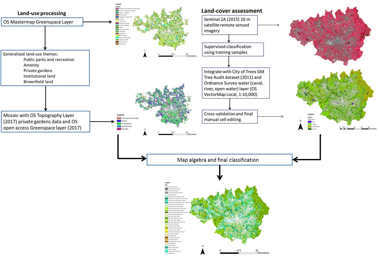
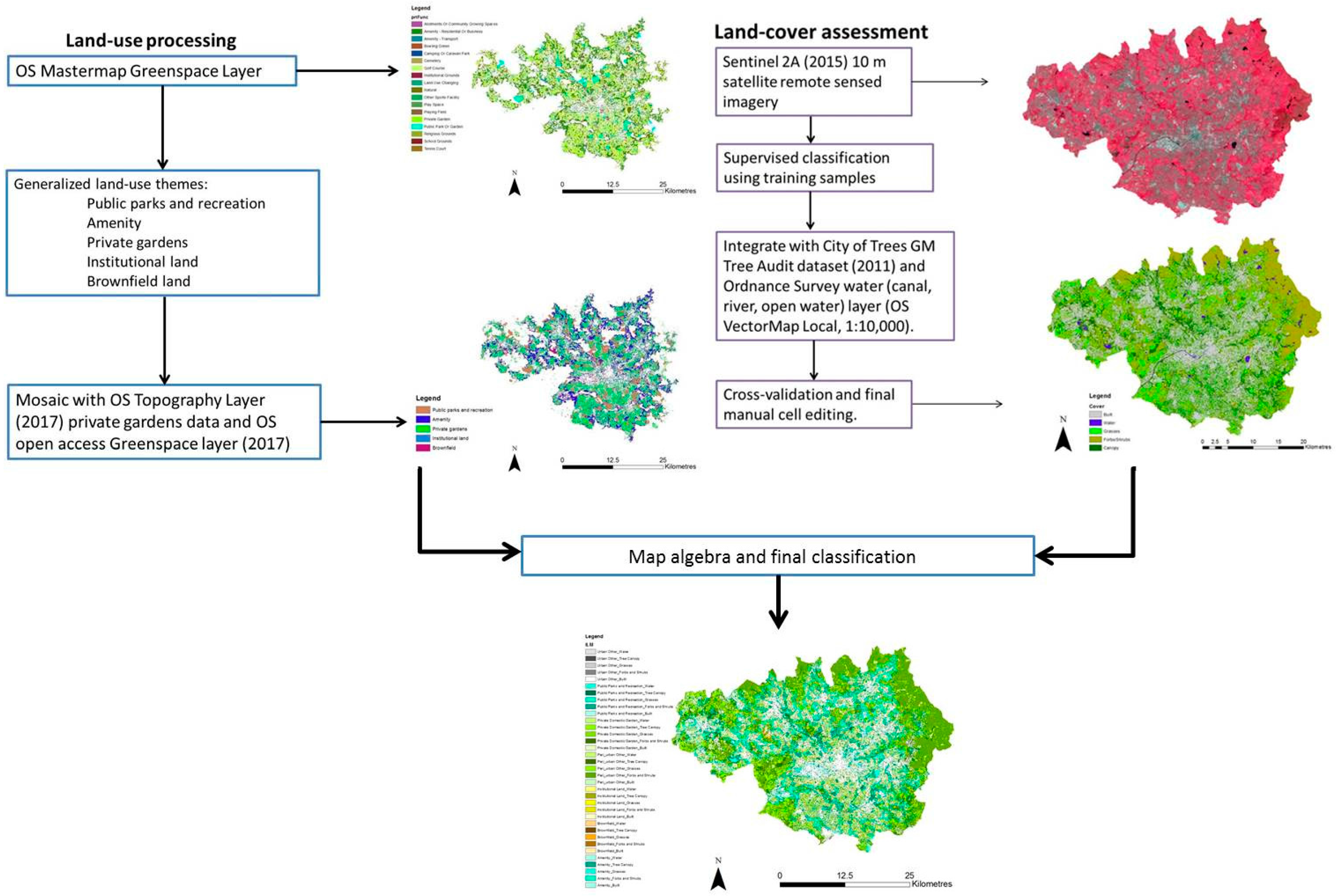
2.1. Overview
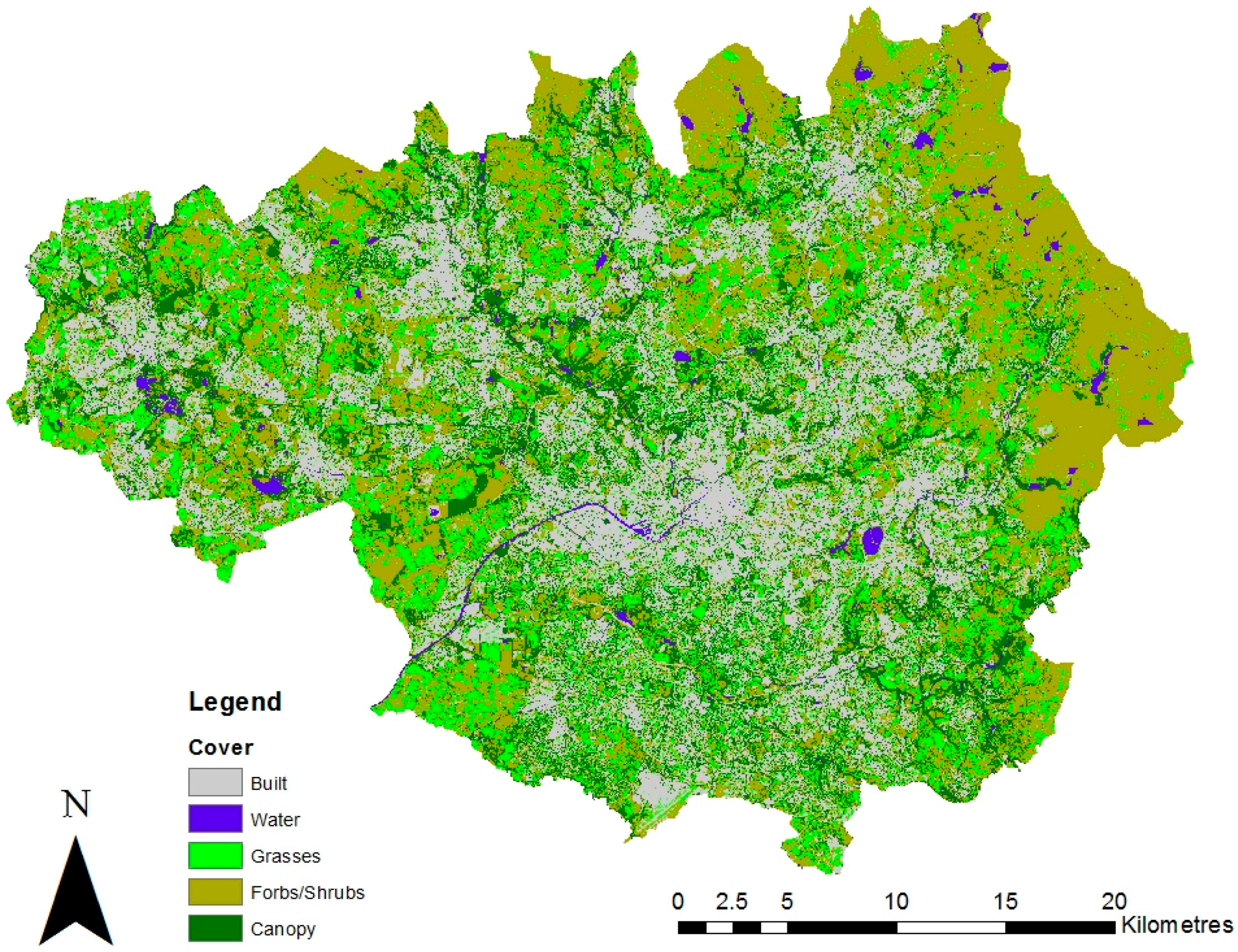
2.2. Stage One: Automatic Land Cover Classification of Sentinel 2A Data and Data Processing
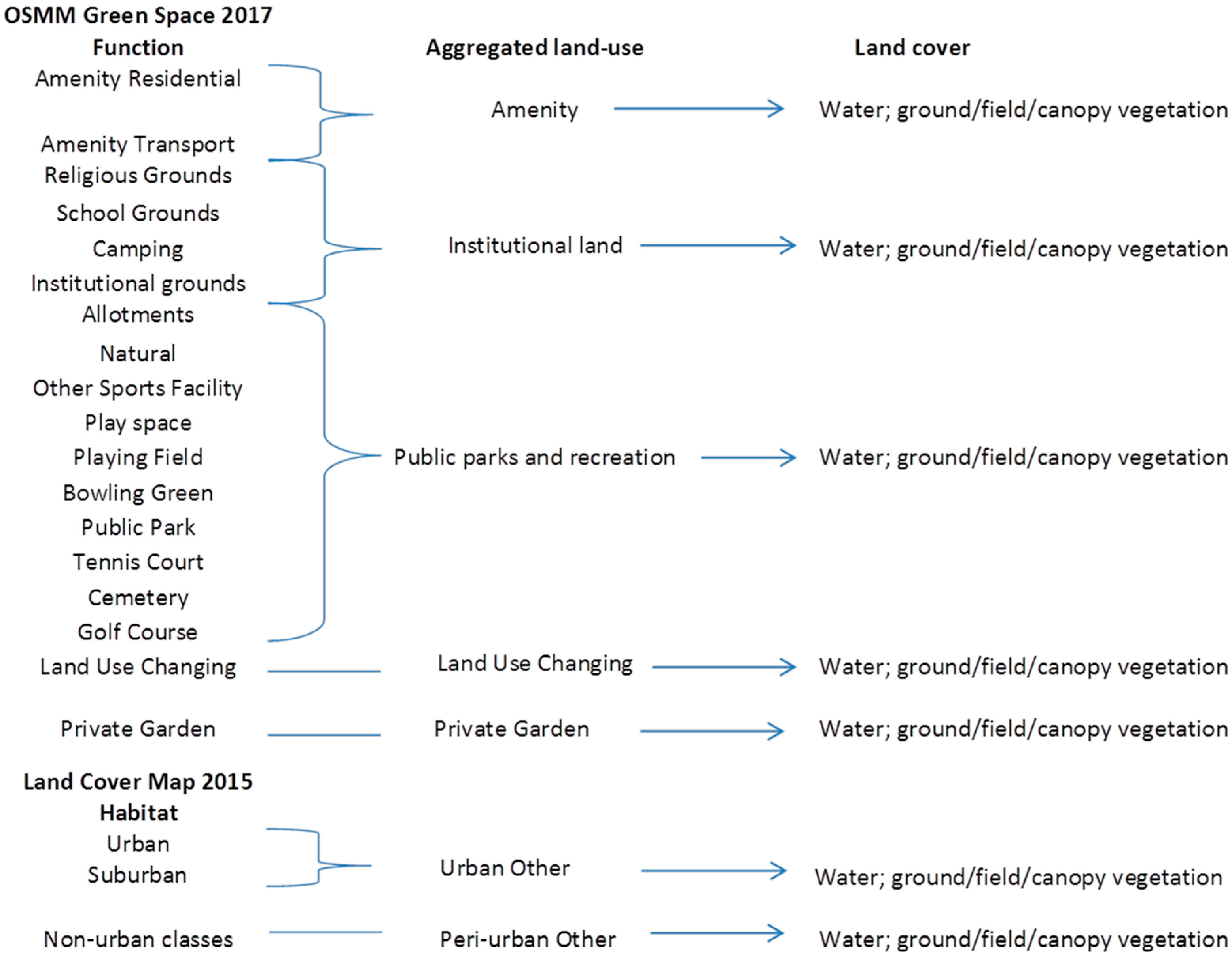
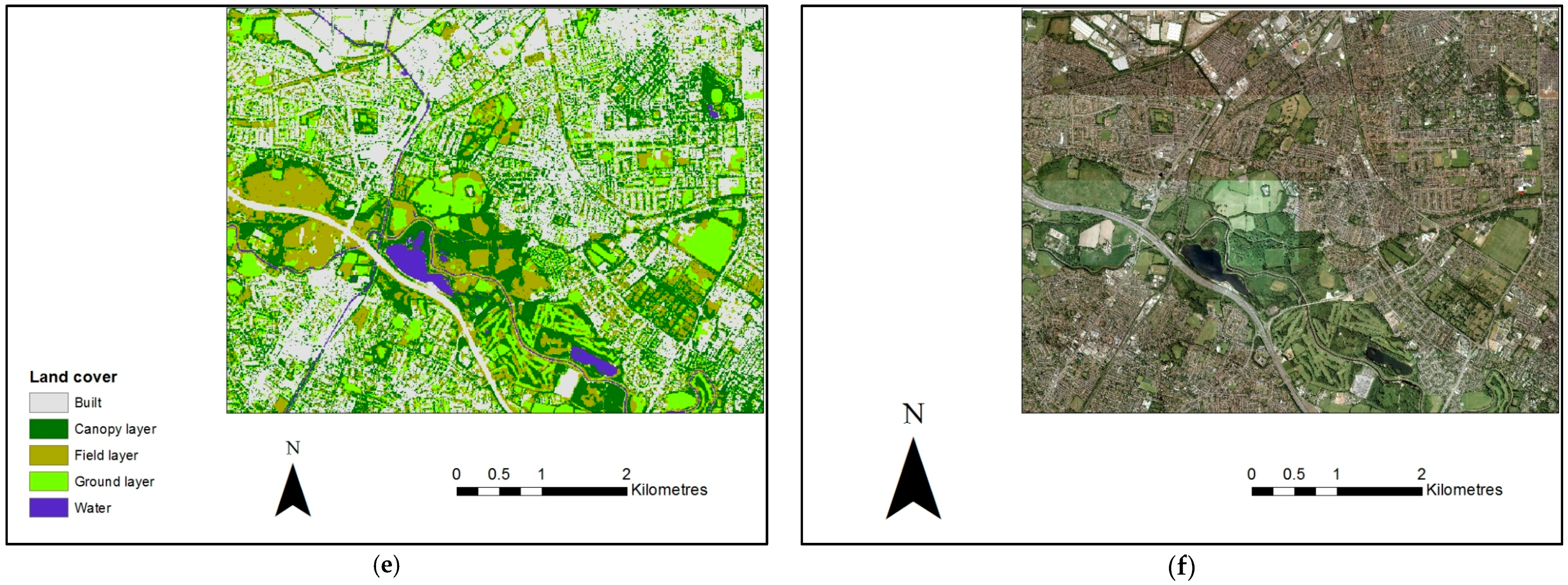
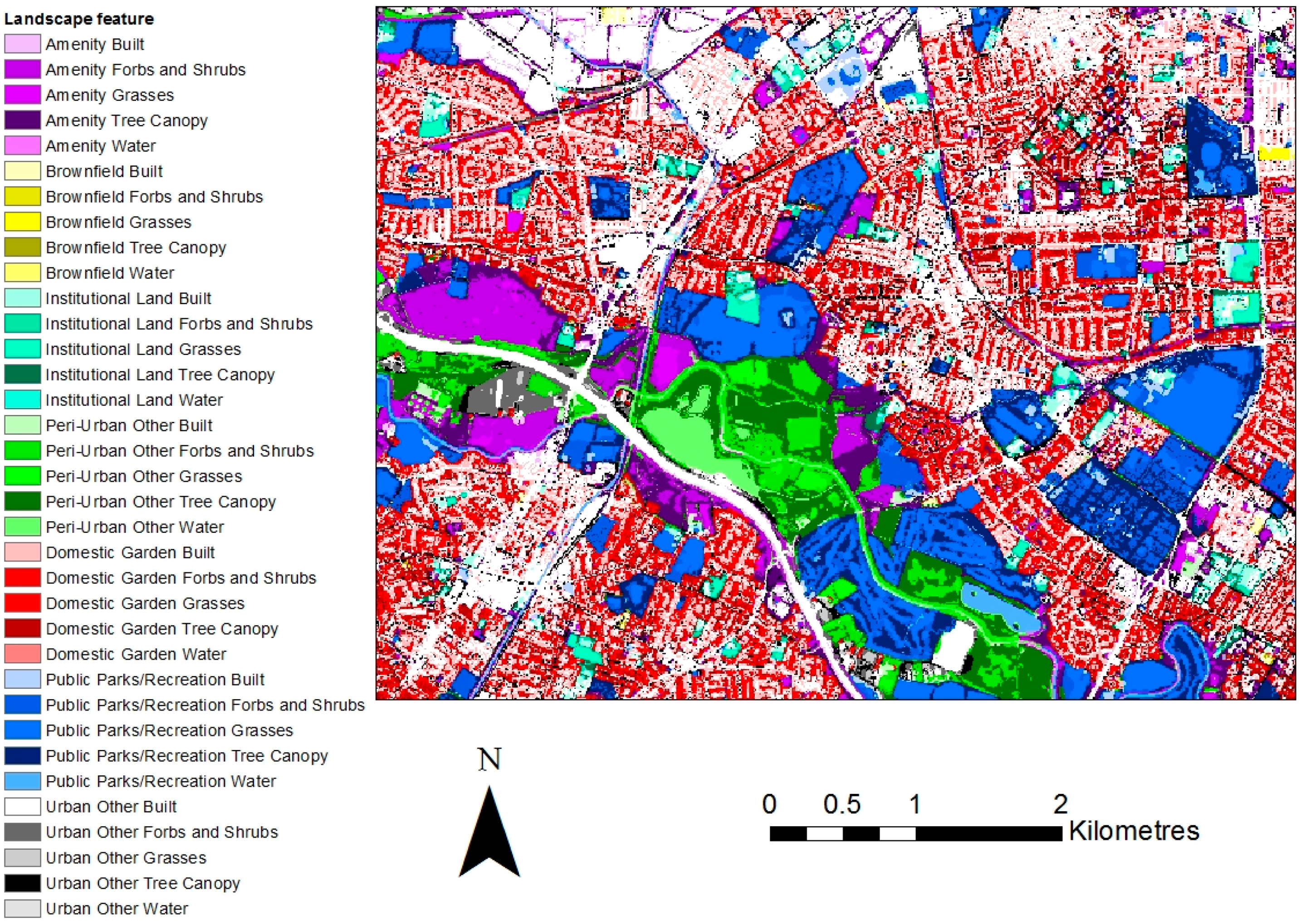
2.3. Stage Two: Generalisation and Incorporation of Land Use Data
2.4. Consideration of Spatial Units
2.5. Stage 3: Validation of the Dataset
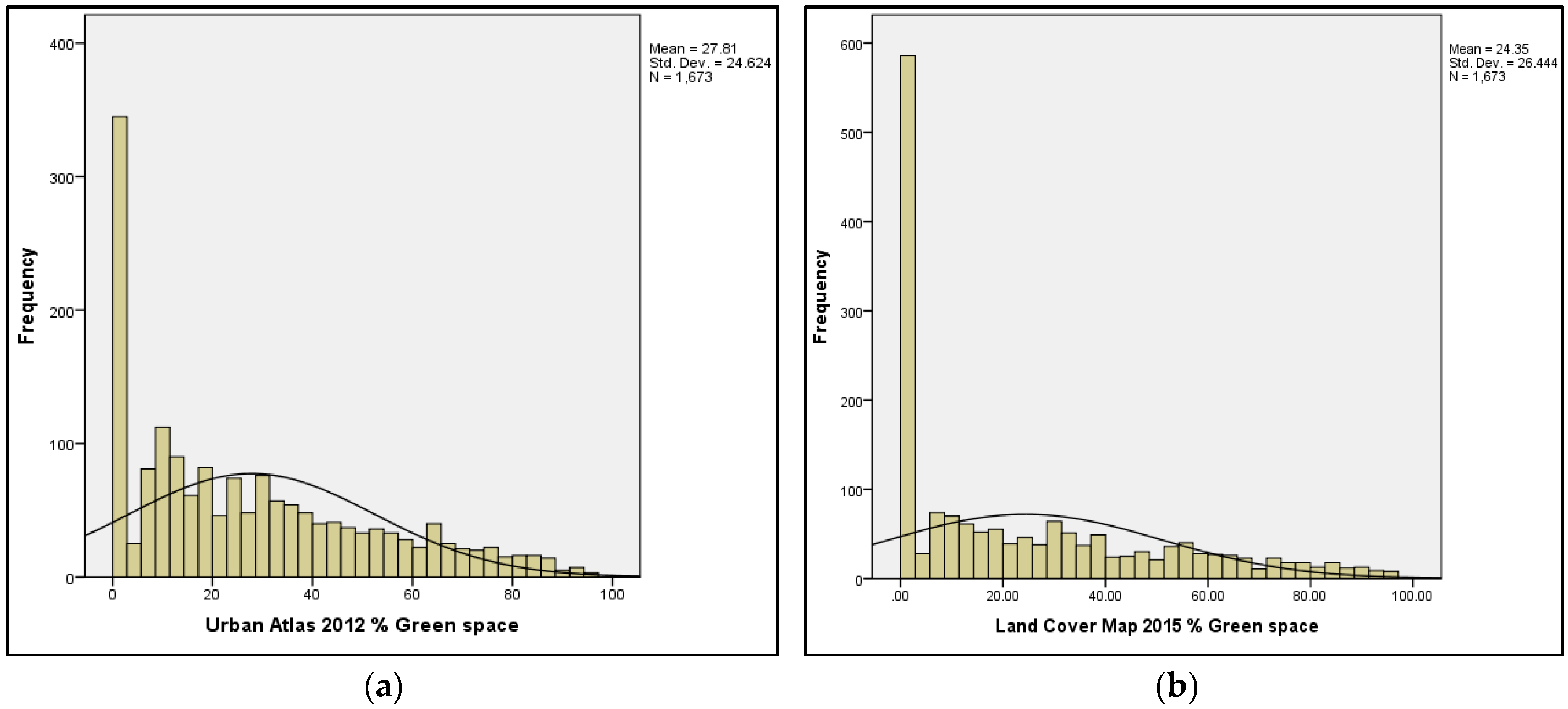
2.5.1. Statistical Comparison with Existing Urban Land Use Data
2.5.2. Calculation of Landscape Indices and Correlations with Socioeconomic and Landscape Characteristics
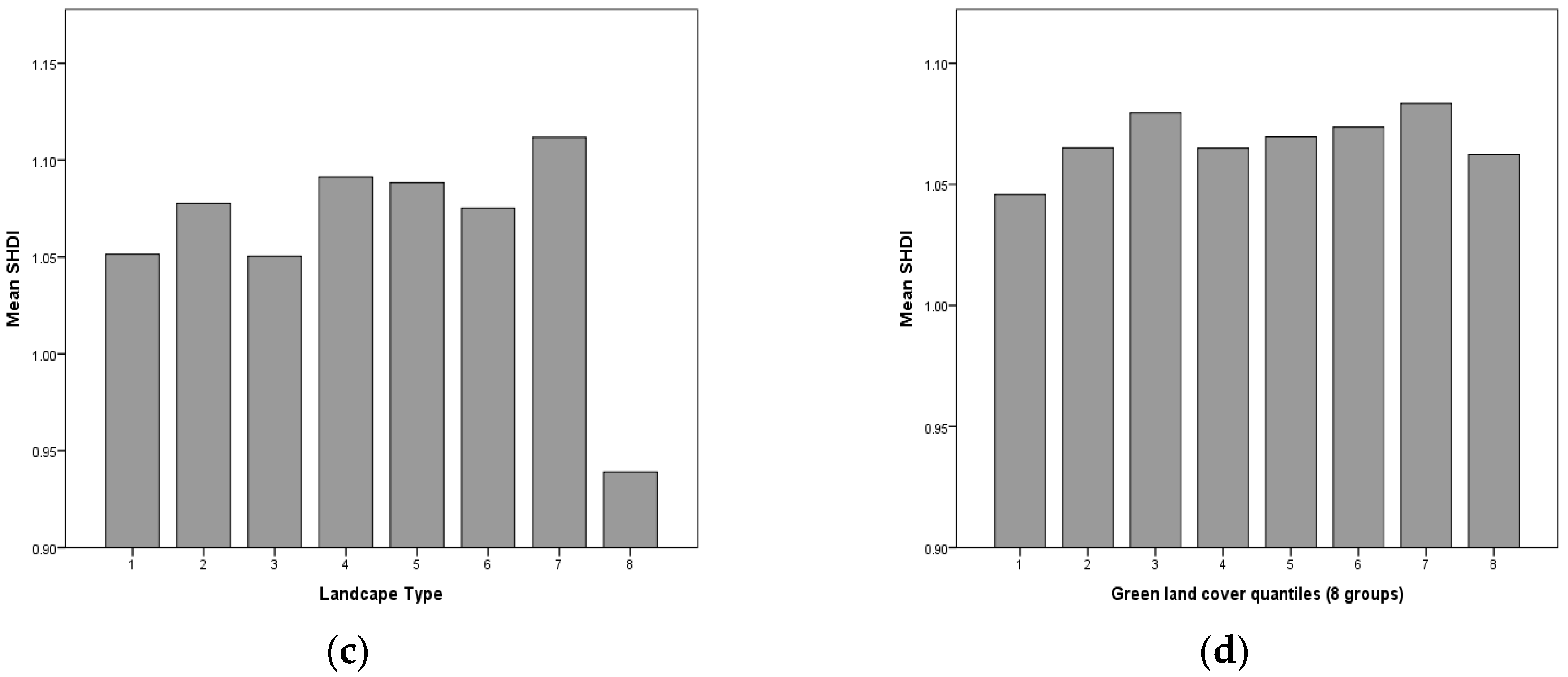
2.5.3. Generation and Assessment of Landscape Types
3. Results
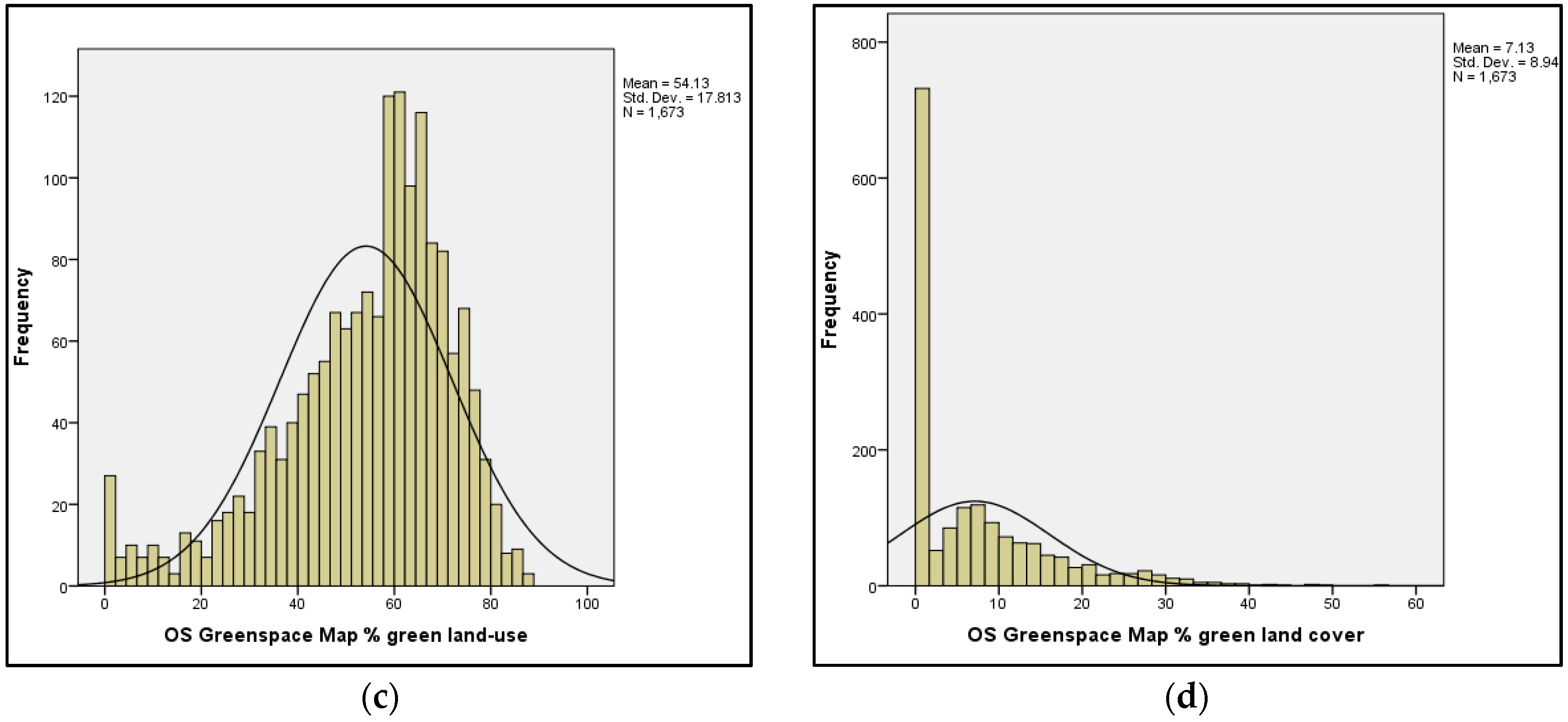
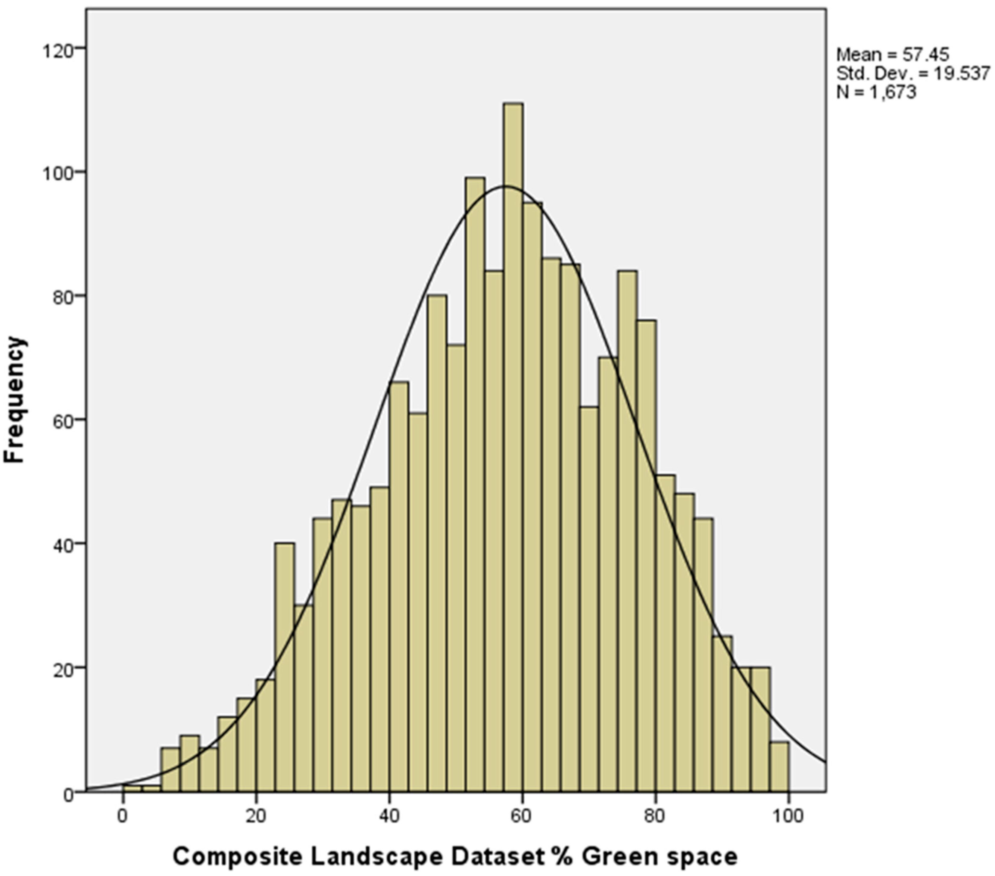
3.1. Statistical Assessment of the Dataset
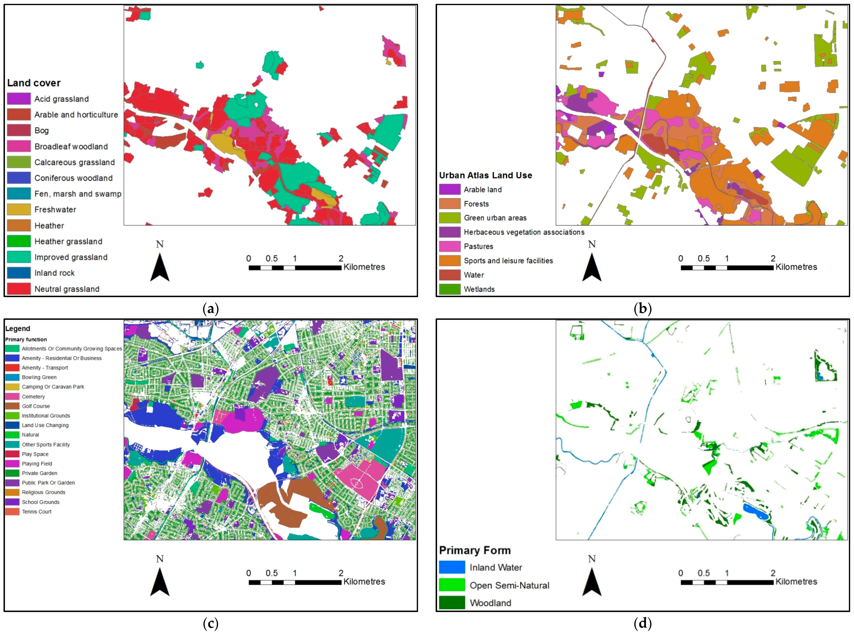
3.2. Final Classification and Exploration of Social–Ecological Relationships
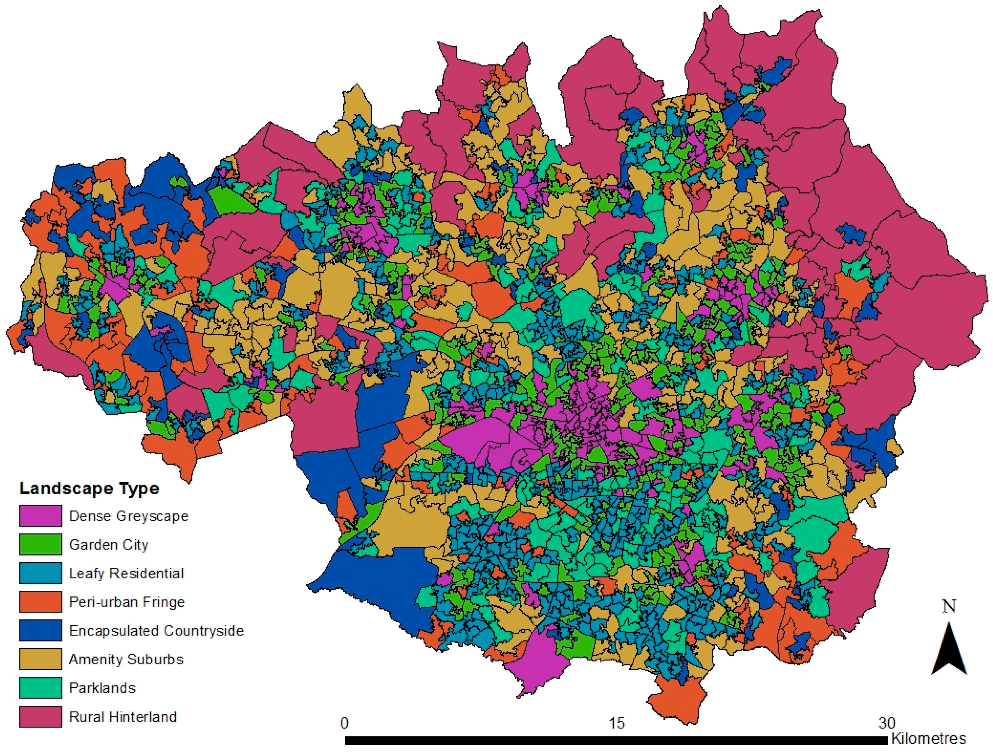
3.3. Development of the Landscape Typology
4. Discussion
5. Conclusions
Supplementary Materials
Acknowledgements
Author Contributions
Conflicts of Interest
References
- De Vries, S.; Verheij, R.A.; Groenewegen, P.P.; Spreeuwenberg, P. Natural environments—Healthy environments? An exploratory analysis of the relationship between greenspace and health. Environ. Plan. A 2003, 35, 1717–1731. [Google Scholar] [CrossRef]
- Mitchell, R.; Popham, F. Greenspace, urbanity and health: Relationships in England. J. Epidemiol. Commun. Health 2007, 61, 681–683. [Google Scholar] [CrossRef] [PubMed]
- Mitchell, R.; Popham, F. Effect of exposure to natural environment on health inequalities: An observational population study. Lancet 2008, 372, 1655–1660. [Google Scholar] [CrossRef]
- Stigsdotter, U.K.; Ekholm, O.; Schipperijn, J.; Toftager, M.; Kamper-Jørgensen, F.; Randrup, T.B. Health promoting outdoor environments-Associations between green space, and health, health-related quality of life and stress based on a Danish national representative survey. Scand. J. Soc. Med. 2010, 38, 411–417. [Google Scholar] [CrossRef] [PubMed]
- Bertram, C.; Rehdanz, K. The role of urban green space for human well-being. Ecol. Econ. 2015, 120, 139–152. [Google Scholar] [CrossRef]
- Jiang, B.; Zhang, T.; Sullivan, W.C. Healthy cities: Mechanisms and research questions regarding the impacts of urban green landscapes on public health and well-being. Landsc. Archit. Front. 2015, 3, 24–36. [Google Scholar]
- Panagopoulos, T.; Duque, J.A.G.; Dan, M.B. Urban planning with respect to environmental quality and human well-being. Environ. Pollut. 2016, 208, 137–144. [Google Scholar] [CrossRef] [PubMed]
- James, P.; Tzoulas, K.; Adams, M.D.; Barber, A.; Box, J.; Breuste, J.; Elmqvist, T.; Frith, M.; Gordon, C.; Greening, K.L.; et al. Towards an integrated understanding of green space in the European built environment. Urban For. Urban Green. 2009, 8, 65–75. [Google Scholar] [CrossRef]
- Thompson, C.W. Linking landscape and health: The recurring theme. Landsc. Urban plan. 2011, 99, 187–195. [Google Scholar] [CrossRef]
- Jennings, V.; Gaither, C.J. Approaching environmental health disparities and green spaces: An ecosystem services perspective. Int. J. Environ. Res. Public Health 2015, 12, 1952–1968. [Google Scholar] [CrossRef] [PubMed]
- Sandifer, P.A.; Sutton-Grier, A.E.; Ward, B.P. Exploring connections among nature, biodiversity, ecosystem services, and human health and well-being: Opportunities to enhance health and biodiversity conservation. Ecosyst. Serv. 2015, 12, 1–15. [Google Scholar] [CrossRef]
- Taylor, W.C.; Floyd, M.F.; Whitt-Glover, M.C.; Brooks, J. Environmental justice: A framework for collaboration between the public health and parks and recreation fields to study disparities in physical activity. J. Phys. Activity Health 2007, 4 (Suppl. 1), S50–S63. [Google Scholar] [CrossRef]
- Jennings, V.; Johnson Gaither, C.; Gragg, R.S. Promoting environmental justice through urban green space access: A synopsis. Environ. Justice 2012, 5, 1–7. [Google Scholar] [CrossRef]
- Wolch, J.R.; Byrne, J.; Newell, J.P. Urban green space, public health, and environmental justice: The challenge of making cities ‘just green enough’. Landsc. Urban Plan. 2014, 125, 234–244. [Google Scholar] [CrossRef]
- Congalton, R.G. A review of assessing accuracy of classifications of remotely sensed data. Remote Sens. Environ. 1991, 37, 35–46. [Google Scholar] [CrossRef]
- Foody, G.M. Approaches for the production and evaluation of fuzzy land cover classifications from remotely sensed data. Int. J. Remote Sens. 1996, 17, 1317–1340. [Google Scholar] [CrossRef]
- Baatz, M.; Schape, A. Object-oriented and multi-scale image analysis in semantic networks. In Proceedings of the 2nd International Symposium on Operationalization of Remote Sensing, Enschede, The Netherlands, 16–20 August 1999. [Google Scholar]
- Turner, M.G.; Gardner, R.H.; O’Neill, R.V. Landscape Ecology Theory and Practice: Pattern and Process; Springer: New York, NY, USA, 2001. [Google Scholar]
- Ju, J.; Kolaczyk, E.D.; Gopal, S. Gaussian mixture discriminant analysis and sub-pixel land cover characterization in remote sensing. Remote Sens. Environ. 2003, 84, 550–560. [Google Scholar] [CrossRef]
- Campbell, J. Introduction to Remote Sensing, 4th ed.; The Guilford Press: New York, NY, USA, 2007. [Google Scholar]
- Lee, A.C.K.; Jordan, H.C.; Horsley, J. Value of urban green spaces in promoting healthy living and wellbeing: Prospects for planning. Risk Manag. Healthc. Policy 2015, 8, 131. [Google Scholar] [CrossRef] [PubMed]
- WHO (World Health Organization). Urban Green Spaces and Health; WHO Regional Office for Europe: Copenhagen, Denmark, 2016. [Google Scholar]
- Benedict, M.A.; McMahon, E.T. Green Infrastructure: Linking Landscapes and Communities; Island Press: Washington, DC, USA, 2012. [Google Scholar]
- TCPA (Town and Country Planning Association). The GRaBS project issue: Green and blue space adaptation for urban areas and eco towns. J. Town Country Plan. Assoc. 2011, 80, 240–299. [Google Scholar]
- Mell, I.C. Can you tell a green field from a cold steel rail? Examining the “green” of Green Infrastructure development. Local Environ. 2013, 18, 152–166. [Google Scholar] [CrossRef]
- Bird, W. Natural greenspace. Br. J. Gen. Pract. 2007, 57, 69. [Google Scholar] [PubMed]
- Ernstson, H. The social production of ecosystem services: A framework for studying environmental justice and ecological complexity in urbanized landscapes. Landsc. Urban Plan. 2013, 109, 7–17. [Google Scholar] [CrossRef]
- Lovell, S.T.; Taylor, J.R. Supplying urban ecosystem services through multifunctional green infrastructure in the United States. Landsc. Ecol. 2013, 28, 1447–1463. [Google Scholar] [CrossRef]
- Armson, D.; Stringer, P.; Ennos, A.R. The effect of tree shade and grass on surface and globe temperatures in an urban area. Urban For. Urban Green. 2012, 11, 245–255. [Google Scholar] [CrossRef]
- Southon, G.E.; Jorgensen, A.; Dunnett, N.; Hoyle, H.; Evans, K.L. Biodiverse perennial meadows have aesthetic value and increase residents’ perceptions of site quality in urban green-space. Landsc. Urban Plan. 2017, 158, 105–118. [Google Scholar] [CrossRef]
- Jacobs, J. The Death and Life of Great American Cities; Random House: New York, NY, USA, 1961. [Google Scholar]
- Baum, F.; Palmer, C. ‘Opportunity structures’: Urban landscape, social capital and health promotion in Australia. Health Promot. Int. 2002, 17, 351–361. [Google Scholar] [CrossRef] [PubMed]
- Niemelä, J. Ecology of urban green spaces: The way forward in answering major research questions. Landsc. Urban Plan. 2014, 125, 298–303. [Google Scholar] [CrossRef]
- Wu, J. Landscape sustainability science: Ecosystem services and human well-being in changing landscapes. Landsc. Ecol. 2013, 28, 999–1023. [Google Scholar] [CrossRef]
- Haase, D.; Larondelle, N.; Andersson, E.; Artmann, M.; Borgström, S.; Breuste, J.; Gomez-Baggethun, E.; Gren, Å.; Hamstead, Z.; Hansen, R.; et al. Quantitative review of urban ecosystem service assessments: Concepts, models, and implementation. Ambio 2014, 43, 413–433. [Google Scholar] [CrossRef] [PubMed]
- Maas, J.; Verheij, R.A.; Groenewegen, P.P.; De Vries, S.; Spreeuwenberg, P. Green space, urbanity, and health: How strong is the relation? J. Epidemiol. Commun. Health 2006, 60, 587–592. [Google Scholar] [CrossRef] [PubMed]
- Maas, J.; Van Dillen, S.M.; Verheij, R.A.; Groenewegen, P.P. Social contacts as a possible mechanism behind the relation between green space and health. Health Place 2009, 15, 586–595. [Google Scholar] [CrossRef] [PubMed]
- Coombes, E.; Jones, A.P.; Hillsdon, M. The relationship of physical activity and overweight to objectively measured green space accessibility and use. Soc. Sci. Med. 2010, 70, 816–822. [Google Scholar] [CrossRef] [PubMed]
- Gill, S.E.; Handley, J.F.; Ennos, A.R.; Pauleit, S.; Theuray, N.; Lindley, S.J. Characterising the urban environment of UK cities and towns: A template for landscape planning. Landsc. Urban Plan. 2008, 87, 210–222. [Google Scholar] [CrossRef]
- Pauleit, S.; Breuste, J.H. Land use and surface cover as urban ecological indicators. In Handbook of Urban Ecology; Oxford University Press: Oxford, UK, 2011; pp. 19–30. [Google Scholar]
- Woldegerima, T.; Yeshitela, K.; Lindley, S. Characterizing the urban environment through urban morphology types (UMTs) mapping and land surface cover analysis: The case of Addis Ababa, Ethiopia. Urban Ecosyst. 2017, 20, 245–263. [Google Scholar] [CrossRef]
- Vatseva, R.; Kopecka, M.; Otahel, J.; Rosina, K.; Kitev, A.; Genchev, S. Mapping urban green spaces based on remote sensing data: Case studies in Bulgaria and Slovakia. In Proceedings of the 6th International Conference on Cartography and Gis, Albena, Bulgaria, 13–17 June 2016; p. 569. [Google Scholar]
- EEA (European Environment Agency). The GMES Urban Atlas. 2012. Available online: http://www.eea.europa.eu/data-and-maps/data/urban-atlas (accessed on 15 June 2017).
- Rowland, C.S.; Morton, R.D.; Carrasco, L.; McShane, G.; O’Neil, A.W.; Wood, C.M. Land Cover Map 2015 (vector, GB). NERC Environmental Information Data Centre. Available online: https://doi.org/10.5285/6c6c9203-7333-4d96-88ab-78925e7a4e73 (accessed on 4 June 2017).
- Botham, M.S.; Rothery, P.; Hulme, P.E.; Hill, M.O.; Preston, C.D.; Roy, D.B. Do urban areas act as foci for the spread of alien plant species? An assessment of temporal trends in the UK. Divers. Distrib. 2009, 15, 338–345. [Google Scholar] [CrossRef]
- Salvati, L.; Ferrara, C. Do changes in vegetation quality precede urban sprawl? Area 2013, 45, 365–375. [Google Scholar] [CrossRef]
- Kuntz, S.; Schmeer, E.; Jochum, M.; Smith, G. Towards an European land cover monitoring service and high-resolution layers. In Land Use and Land Cover Mapping in Europe; Springer: Dordrecht, The Netherlands, 2014; pp. 43–52. [Google Scholar]
- Trigila, A.; Iadanza, C.; Munafò, M.; Marinosci, I. Population exposed to landslide and flood risk in Italy. In Engineering Geology for Society and Territory-Volume 5; Springer: Cham, Switzerland, 2015; pp. 843–848. [Google Scholar]
- Sapena, M.; Ruiz, L.A. Analysis of urban development by means of multi-temporal fragmentation metrics from LULC data. Int. Arch. Photogr. Remote Sens. Spat. Inf. Sci. 2015, 40, 1411. [Google Scholar] [CrossRef]
- Beloconi, A.; Kamarianakis, Y.; Chrysoulakis, N. Estimating urban PM10 and PM2.5 concentrations, based on synergistic MERIS/AATSR aerosol observations, land cover and morphology data. Remote Sens. Environ. 2016, 172, 148–164. [Google Scholar] [CrossRef]
- Margaritis, E.; Kang, J. Relationship between green space-related morphology and noise pollution. Ecol. Indic. 2017, 72, 921–933. [Google Scholar] [CrossRef]
- OS MasterMap Greenspace Layer [Shape Geospatial Data], Scale 1:1250, Tile(s): Greater Manchester, Updated: July 2017, Ordnance Survey, Using: EDINA Digimap Ordnance Survey Service. Available online: http://digimap.edina.ac.uk (accessed on 26 July 2017).
- OS Open Green Space [Shape Geospatial Data], Scale 1:2500, Tile(s): Greater Manchester, Updated: July 2017, Ordnance Survey, Using: EDINA Digimap Ordnance Survey Service. Available online: http://digimap.edina.ac.uk/ (accessed on 26 July 2017).
- European Space Agency. Copernicus Sentinel Data. 2015. Available online: https://scihub.copernicus.eu/dhus (accessed on 25 October 2016).
- Greatermanchester-ca.gov.uk. Greater Manchester Combined Authority|GMCA. 2018. Available online: https://www.greatermanchester-ca.gov.uk/about (accessed 23 January 2018).
- Rosina, K.; Kopecká, M. Mapping of urban green spaces using Sentinel-2A data: Methodical aspects. In Proceedings of the 6th International Conference on Cartography and Gis, Albena, Bulgaria, 13–17 June 2016; p. 562. [Google Scholar]
- Cityoftrees.org.uk; Greater Manchester Tree Audit [computer file]. (Manchester, UK). Personal communication, 2011.
- OS Open Rivers [Shape Geospatial Data], Scale 1:15,000, Tile(s): Greater Manchester, Updated: July 2017, Ordnance Survey, Using: EDINA Digimap Ordnance Survey Service. Available online: http://digimap.edina.ac.uk/ (accessed on 26 July 2017).
- Edina 2017, Scale 1:500, Tile(s): Manchester, Updated: 2015, Getmapping Plc, Using: EDINA Digimap Ordnance Survey Service. Available online: http://digimap.edina.ac.uk (accessed on 17 September 2017).
- OS MasterMap Topography Layer [Shape geospatial data], Scale 1:1250, Tile(s): Greater Manchester, Updated: July 2017, Ordnance Survey, Using: EDINA Digimap Ordnance Survey Service. Available online: http://digimap.edina.ac.uk/ (accessed on 11 July 2017).
- ONS (Office for National Statistics). Available online: https://www.ons.gov.uk/methodology/geography/ukgeographies/censusgeography (accessed on 22 July 2017).
- ONS (Office for National Statistics). 2011 Census: Digitised Boundary Data (England and Wales) [computer file]. UK Data Service Census Support. Available online: http://edina.ac.uk/census. Licensed under the terms of the Open Government Licence. Available online: http://www.nationalarchives.gov.uk/doc/open-government-licence/version/2 (accessed on 1 July 2017).
- Jung, M. LecoS—A python plugin for automated landscape ecology analysis. Ecol. Inform. 2016, 31, 18–21. [Google Scholar] [CrossRef]
- Li, F.; Liu, X.; Zhang, X.; Zhao, D.; Liu, H.; Zhou, C.; Wang, R. Urban ecological infrastructure: An integrated network for ecosystem services and sustainable urban systems. J. Clean. Prod. 2017, 136, S12–S18. [Google Scholar] [CrossRef]
- DCLG (Department for Communities and Local Government). English Indices of Deprivation 2015 [Computer File]. Available online: https://www.gov.uk/government/statistics/english-indices-of-deprivation-2015. Licensed Under. Available online: https://www.nationalarchives.gov.uk/doc/open-government-licence/version/3 (accessed on 20 October 2016).
- Lance, G.N.; Williams, W.T. A general theory of classificatory sorting strategies: II. Clustering systems. Comput. J. 1967, 10, 271–277. [Google Scholar] [CrossRef]
- Foody, G.M. Status of land cover classification accuracy assessment. Remote Sens. Environ. 2002, 80, 185–201. [Google Scholar] [CrossRef]
- Biro, K.; Pradhan, B.; Buchroithner, M.; Makeschin, F. Use of multi-temporal satellite data for land-use/Land-cover change analyses and its impacts on soil properties in the northern part of Gadarif Region. In Remote Sensing for Science, Education, and Natural and Cultural Heritage; Reuter, R., Ed.; EARSel: Paris, France, 2010; pp. 305–312. [Google Scholar]
- Dennis, M.; James, P. User participation in urban green commons: Exploring the links between access, voluntarism, biodiversity and well being. Urban For. Urban Green. 2016, 15, 22–31. [Google Scholar] [CrossRef]
- Dennis, M.; James, P. Evaluating the relative influence on population health of domestic gardens and green space along a rural-urban gradient. Landsc. Urban Plan. 2017, 157, 343–351. [Google Scholar] [CrossRef]
- Dennis, M.; James, P. Site-specific factors in the production of local urban ecosystem services: A case study of community-managed green space. Ecosyst. Serv. 2016, 17, 208–216. [Google Scholar] [CrossRef]
- Speak, A.F.; Mizgajski, A.; Borysiak, J. Allotment gardens and parks: Provision of ecosystem services with an emphasis on biodiversity. Urban For. Urban Green. 2015, 14, 772–781. [Google Scholar] [CrossRef]
- Dennis, M.; James, P. Ecosystem services of collectively managed urban gardens: Exploring factors affecting synergies and trade-offs at the site level. Ecosyst. Serv. 2017, 26, 17–26. [Google Scholar] [CrossRef]
- Armitage, D.; Béné, C.; Charles, A.; Johnson, D.; Allison, E. The interplay of well-being and resilience in applying a social-ecological perspective. Ecol. Soc. 2012, 17. [Google Scholar] [CrossRef]
- Eurogeographics.org. 2018 Members|EuroGeographics. Available online: http://www.eurogeographics.org/about/members (accessed on 16 January 2018).


| Urban Atlas | Corine Land Cover | Land Cover Map | |
|---|---|---|---|
| Minimum mapping units | 0.25 ha | 25 ha | 0.5 ha |
| Input data resolution | 2.5 m | 25 m | 25 m |
| Available years | 2006; 2012 | 1990; 2000; 2006; 2012 | 2007; 2015 |
| Number of land use/land cover classes | 27 | 44 | 21 |
| Thematic accuracy | ≥80% | ≥85% | - |
| Control Variable: Income Deprivation Score | Public Parks and Recreation Grasses | Public Parks and Recreation Forbs and Shrubs | Public Parks and Recreation Tree Canopy | Amenity Grasses | Amenity Forbs and Shrubs | Amenity Trees | Private Garden Grasses | Private Garden Forbs and Shrubs | Private Garden Trees | ||
|---|---|---|---|---|---|---|---|---|---|---|---|
| Years of potential life lost indicator | Correlation | −0.066 * | −0.074 * | −0.026 | −0.102 * | −0.109 * | −0.036 | −0.176 * | −0.263 * | −0.132 * | |
| Significance (2-tailed) | 0.007 | 0.002 | 0.285 | 0.000 | 0.000 | 0.139 | 0.000 | 0.000 | 0.000 | ||
| Peri-Urban Other: Tree Canopy | Brownfield: Tree Canopy | Institutional Land: Tree Canopy | Private Domestic Garden: Tree Canopy | Amenity: Tree Canopy | Public Parks and Recreation: Tree Canopy | Other Urban: Tree Canopy | ||
|---|---|---|---|---|---|---|---|---|
| LD | Correlation Coefficient | −095 * | 0.062 * | 0.082 * | −0.201 * | −0.218 * | 0.257 * | 0.253 * |
| Sig. (2-tailed) | 0.000 | 0.012 | 0.001 | 0.000 | 0.000 | 0.000 | 0.000 | |
| Canopy ENN | Correlation Coefficient | 0.066 * | 0.158 * | −0.049* | −0.313 * | 0.274 * | 0.274* | −0.283 * |
| Sig. (2-tailed) | 0.007 | 0.000 | 0.046 | 0.000 | 0.000 | 0.000 | 0.000 | |
| Percentage Cover LSOA−¹ | |||||||||||||||
|---|---|---|---|---|---|---|---|---|---|---|---|---|---|---|---|
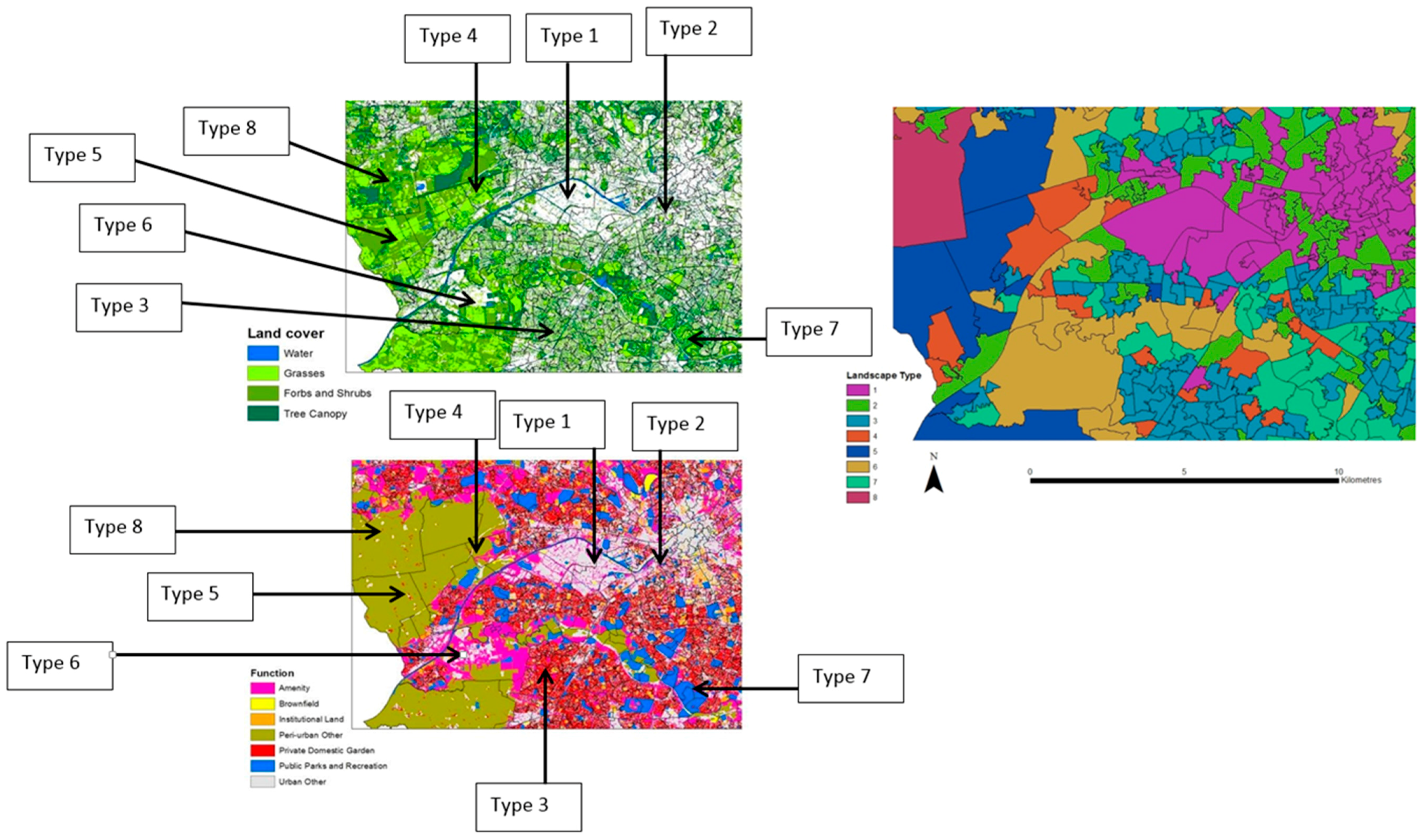
| Landscape Type with Indicative Labels | Public | Amenity | Gardens | Peri-Urban | Institutional Land | Brownfield Land | Urban Other | Grasses | Forbs & Shrubs | Canopy | Green/Blue Cover | SHDI | LD | ||
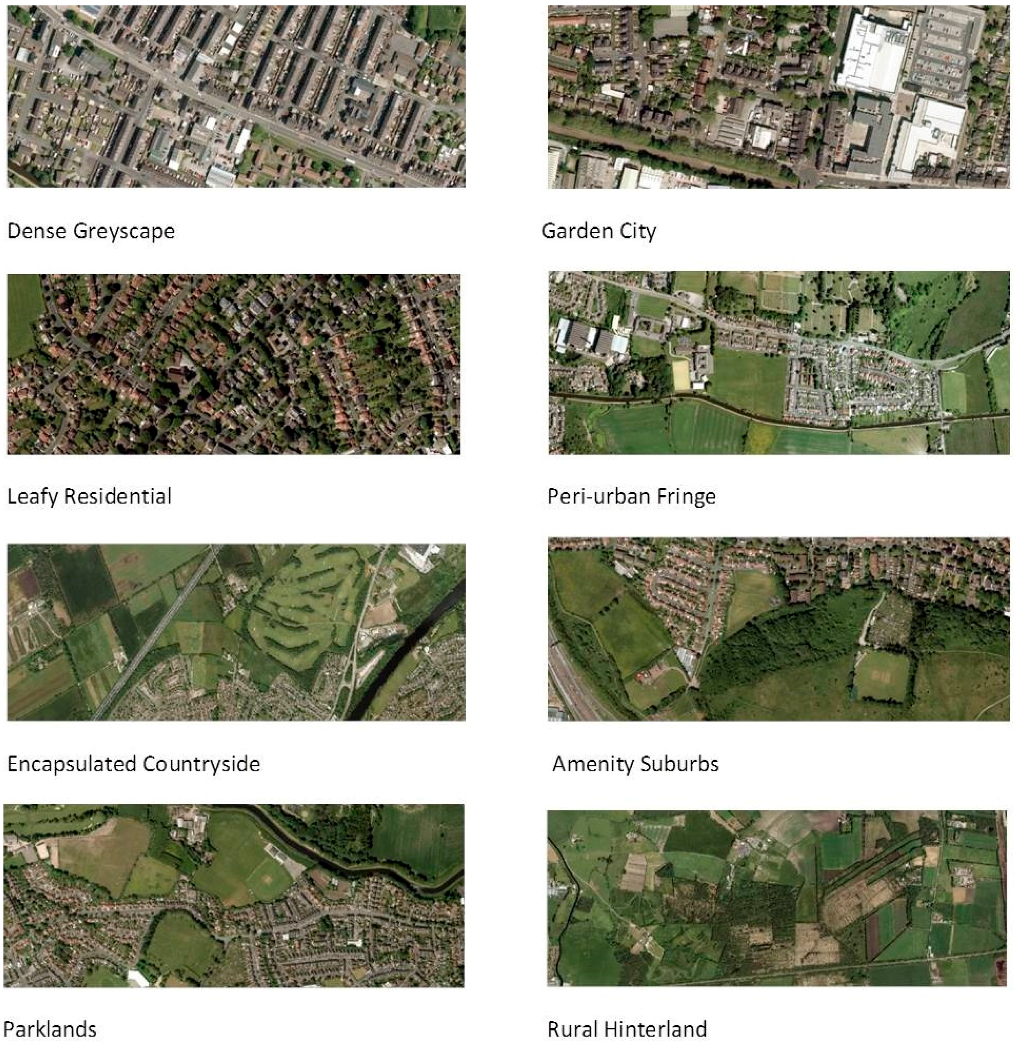
| Dense Greyscape | Highly urbanised; very high population density; very low green space cover, high proportion amenity | Mean | 4.32 | 10.71 | 14.53 | 1.27 | 3.75 | 1.04 | 64.38 | 4.8 | 6.3 | 12.55 | 25.04 | 1.051 | 0.783 |
| SD | 4.32 | 6.86 | 8.95 | 2.62 | 4.79 | 2.37 | 9.55 | 2.32 | 3.96 | 5.19 | 9.53 | 0.148 | 0.16 | ||
| N | 171 | 171 | 171 | 171 | 171 | 171 | 171 | 171 | 171 | 171 | 171 | 171 | 171 | ||
| Garden city | High population density, moderate cover by domestic gardens, high surface sealing | Mean | 9.17 | 12.86 | 28.09 | 2.97 | 4.16 | 0.71 | 42.05 | 9.93 | 13.14 | 19.33 | 43.36 | 1.078 | 0.596 |
| SD | 7.67 | 7.64 | 9.15 | 5.51 | 5.3 | 2.37 | 7.33 | 4.06 | 5.4 | 6.08 | 9.49 | 0.106 | 0.207 | ||
| N | 309 | 309 | 309 | 309 | 309 | 309 | 309 | 309 | 309 | 309 | 309 | 309 | 309 | ||
| Leafy Residential | Leafy residential areas, high canopy cover | Mean | 5.75 | 9.51 | 53.55 | 2.34 | 3.79 | 0.16 | 24.91 | 14.42 | 16.89 | 25.11 | 56.75 | 1.05 | 0.391 |
| SD | 6.54 | 7.06 | 8.84 | 4.14 | 4.71 | 0.7 | 6.85 | 5.51 | 5.74 | 8.51 | 11.37 | 0.076 | 0.273 | ||
| N | 445 | 445 | 445 | 445 | 445 | 445 | 445 | 445 | 445 | 445 | 445 | 444 | 444 | ||
| Peri-urban Fringe | Urban fringe; low density residential; moderate canopy and overall green cover | Mean | 7.42 | 9.69 | 22.06 | 42.78 | 1.71 | 0.27 | 16.08 | 18.46 | 22.69 | 22.7 | 65.29 | 1.091 | 0.325 |
| SD | 7.98 | 8.3 | 9.63 | 10.68 | 2.59 | 1.05 | 8.53 | 9.56 | 9.42 | 8.59 | 17.69 | 0.083 | 0.274 | ||
| N | 151 | 151 | 151 | 151 | 151 | 151 | 151 | 151 | 151 | 151 | 151 | 151 | 151 | ||
| Encapsulated Countryside | Peri-urban vegetation; extensive informal grassland and wooded areas; very low garden; amenity of formal green space. | Mean | 2.15 | 4.02 | 7.32 | 80.1 | 0.45 | 0.16 | 5.8 | 16.4 | 26.11 | 21.47 | 65.83 | 1.088 | 0.321 |
| SD | 2.93 | 4.66 | 4.26 | 10.17 | 0.8 | 1.12 | 4.28 | 8.78 | 11.95 | 8.99 | 18.7 | 0.102 | 0.277 | ||
| N | 88 | 88 | 88 | 88 | 88 | 88 | 88 | 88 | 88 | 88 | 88 | 88 | 88 | ||
| Amenity Suburbs | Very high provision of amenity greenery; low density residential areas with high cover by trees and higher plants. | Mean | 7.23 | 36.76 | 25.86 | 7.81 | 2.81 | 0.62 | 18.9 | 15.01 | 28.57 | 25.76 | 70.78 | 1.075 | 0.259 |
| SD | 6.42 | 10.61 | 10.38 | 7.62 | 3.99 | 3.18 | 7.78 | 6.53 | 9.61 | 9.66 | 10.17 | 0.09 | 0.203 | ||
| N | 287 | 287 | 287 | 287 | 287 | 287 | 287 | 287 | 287 | 287 | 287 | 287 | 287 | ||
| Parklands | High formal public green space provision; extensive canopy and overall green cover | Mean | 39.13 | 10.97 | 25.92 | 4.56 | 2.6 | 0.26 | 16.55 | 17.67 | 22.93 | 30.34 | 73.51 | 1.112 | 0.214 |
| SD | 12.28 | 7.6 | 10.69 | 6.78 | 4.31 | 0.83 | 7.3 | 7.22 | 7.29 | 9.49 | 10.89 | 0.092 | 0.193 | ||
| N | 168 | 168 | 168 | 168 | 168 | 168 | 168 | 168 | 168 | 168 | 168 | 168 | 168 | ||
| Rural Hinterland | Semi-rural areas dominated by open pasture and grassland | Mean | 7.91 | 17.53 | 11.43 | 51.7 | 0.99 | 0.23 | 10.22 | 18.91 | 57.36 | 12.41 | 90.01 | 0.939 | 0.104 |
| SD | 8.24 | 11.44 | 4.75 | 14.38 | 1.63 | 0.67 | 5.47 | 7.89 | 14.36 | 5.36 | 6.97 | 0.136 | 0.166 | ||
| N | 54 | 54 | 54 | 54 | 54 | 54 | 54 | 54 | 54 | 54 | 54 | 54 | 54 | ||
© 2018 by the authors. Licensee MDPI, Basel, Switzerland. This article is an open access article distributed under the terms and conditions of the Creative Commons Attribution (CC BY) license (http://creativecommons.org/licenses/by/4.0/).
Share and Cite
Dennis, M.; Barlow, D.; Cavan, G.; Cook, P.A.; Gilchrist, A.; Handley, J.; James, P.; Thompson, J.; Tzoulas, K.; Wheater, C.P.; et al. Mapping Urban Green Infrastructure: A Novel Landscape-Based Approach to Incorporating Land Use and Land Cover in the Mapping of Human-Dominated Systems. Land 2018, 7, 17. https://doi.org/10.3390/land7010017
Dennis M, Barlow D, Cavan G, Cook PA, Gilchrist A, Handley J, James P, Thompson J, Tzoulas K, Wheater CP, et al. Mapping Urban Green Infrastructure: A Novel Landscape-Based Approach to Incorporating Land Use and Land Cover in the Mapping of Human-Dominated Systems. Land. 2018; 7(1):17. https://doi.org/10.3390/land7010017
Chicago/Turabian StyleDennis, Matthew, David Barlow, Gina Cavan, Penny A. Cook, Anna Gilchrist, John Handley, Philip James, Jessica Thompson, Konstantinos Tzoulas, C. Philip Wheater, and et al. 2018. "Mapping Urban Green Infrastructure: A Novel Landscape-Based Approach to Incorporating Land Use and Land Cover in the Mapping of Human-Dominated Systems" Land 7, no. 1: 17. https://doi.org/10.3390/land7010017