Real-Time Video Stitching Using Camera Path Estimation and Homography Refinement

1
Department of Electronics Engineering, Kyung Hee University, Yongin 17104, Korea
2
Humanitas College, Kyung Hee University, Yongin 17104, Korea
*
Author to whom correspondence should be addressed.
Symmetry 2018, 10(1), 4; https://doi.org/10.3390/sym10010004
Submission received: 1 December 2017
/
Revised: 20 December 2017
/
Accepted: 25 December 2017
/
Published: 26 December 2017
Abstract
:We propose a novel real-time video stitching method using camera path estimation and homography refinement. The method can stably stitch multiple frames acquired from moving cameras in real time. In the proposed method, one initial between-camera (BC) homography and each camera path (CP) homography are used to estimate the BC homography at every frame. The BC homography is refined by using block matching to adjust the errors of estimated CPs (homography refinement). For fast processing, we extract features using the difference of intensities and use the optical flow to estimate camera motion (CM) homographies, which are multiplied with the previous CMs to calculate CPs (camera path estimations). In experiments, we demonstrated the performance of the CP estimation and homography refinement approach by comparing it with other methods. The experimental results show that the proposed method can stably stitch two image sequences at a rate exceeding 13 fps (frames per second).
1. Introduction
Video stitching is a technique that stitches multiple videos acquired from moving cameras. By allowing the videos to have a wider field of view (FOV) and higher a resolution, users can be immersed in the video. Video stitching has been applied in various fields, including surveillance systems [1,2,3], teleconferencing, immersive virtual reality, and sports broadcasting.
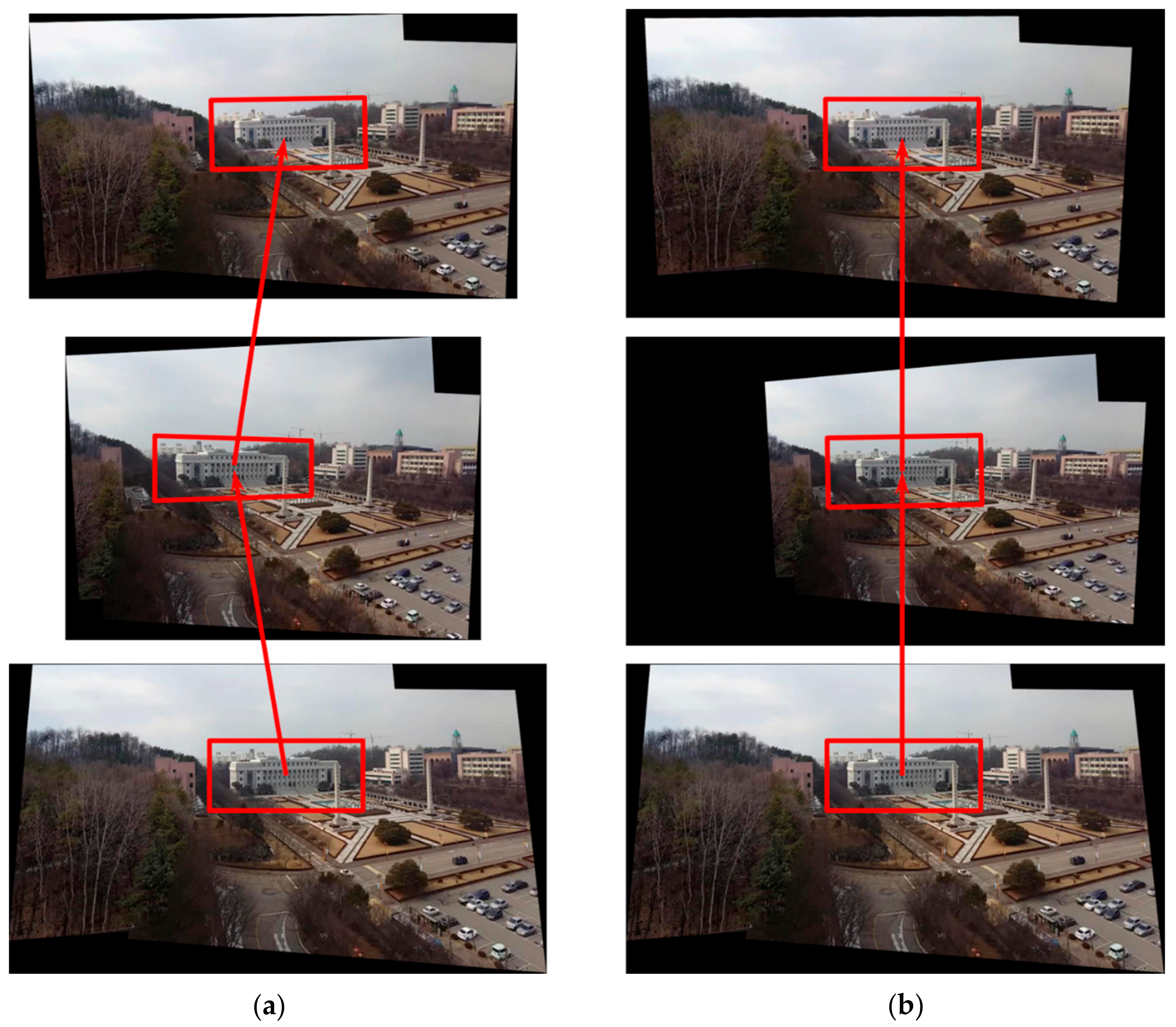
Most video stitching methods are for cameras mounted on fixed rigs [4]. The use of fixed rigs is advantageous in that the processing time is short by using a fixed homography. However, it is difficult for the general public to utilize these approaches due to the expensive camera systems. Recently, video stitching methods for mobile devices, which are cheaper than these camera systems, have been proposed. Lin [5] and Guo’s [6] methods use camera paths (CPs), which are the products of the consecutive camera motion (CM) homographies, but do not rely on direct computations of homographies. This method is very stable for moving cameras, as shown in Figure 1.
Though video stitching using CPs has acceptable performance, this approach has two problems. First, this method requires excessive processing time. The above two methods cannot be used for processing in a real-time system, because a conventional PC takes 3–4 s to stitch two frames for a video with a resolution of 1280 × 720 pixels. Second, misalignments are observed by successive compounding errors. The stitching method using CPs estimates the between-camera (BC) homography through the products of the initial BC homography and CPs. Therefore, in case that the errors of CPs occur, the misaligned artifacts are included in the results.
This paper is aimed at resolving these two central problems of earlier video stitching algorithms. To achieve this goal, we propose CP estimation and homography refinement. The CP estimation is a fast homography estimation method. The CP estimation uses difference of intensity on the grid and Lucas–Kanade optical flow [7] to estimate CPs, instead of using existing methods [8], which consist of three steps: feature extraction (SIFT [9], SURF [10]), feature matching (FLANN [11]), and homography estimation (RANSAC [12]), that takes a relatively long time. The homography refinement is a method for adjusting the errors of BC estimation. The refined BCs are updated by multiplying by the inverse of the error motions, which are estimated by block matching.
In this paper, we propose real-time video stitching using CP estimation and homography refinement. In the experiment, we measure the processing time and stitching score with various samples with a resolution of 1280 × 720 pixels. The experimental results show that the proposed method can stitch two video frames in real-time at a rate exceeding 13 fps (frames per second).
The rest of this paper is organized as follows. Section 2 reviews earlier related works. Section 3 presents an overview of our methods. Section 4 presents the CP estimation in detail. Section 5 also presents the homography refinements. Experiments are presented in Section 6. A larger discussion is provided in Section 7. Finally, summarizing conclusions are drawn in Section 8.
2. Related Work
2.1. Image Stitching
We will review prominent existing image stitching research. The outstanding issue of image stitching is how to remove the misalignments that are generated by parallaxes. Researchers have attempted various approaches to solve the problems mentioned above. The research has generally focused on two approaches: (1) seam-driven methods [13,14,15,16], and (2) warping methods [17,18,19,20]. First, seam-driven methods are techniques that find the optimal seam that separates two images to minimize the stitching errors. Many diverse methods to find the optimal seam have been studied. Agarwala [13] found the seam by using a graph-cut. Gao [14] selected the best seam among the seam candidates that are generated by various homographies. Zomet [15] proposed gradient domain image stitching (GIST), which minimizes the cost functions of the gradient domain. Lee [16] proposed the use of structure deformation using the histogram of gradient (HoG) along the seams. Second, warping methods are techniques that warp the images generated by multiple homographies instead of estimating a global homography. Gao [17] proposed a warping method using a dual-homography that is a combination of a distance plane and a ground plane with corresponding weight maps. Lin [18] generated smoothly varying affine models to handle the parallax in the images. Zaragoza [19] proposed the as-projective-as-possible (APAP) method with a moving direct linear transformation (DLT), which is a warping method that aims to obtain the global homography while allowing the existence of local non-projective deviations. Chang’s [20] approach used a spatial combination of the perspective and a similarity transformation.
2.2. Video Stitching
Research in the field of video stitching can broadly be divided into two categories: (1) misalignment removal, and (2) processing time reduction. First, the processing of misalignment removal is itself an important issue in video stitching. To remove misalignment, most papers refer to ideas employed in image stitching. Some of these papers used seam-driven methods. He’s [1] group proposed use of the seam selection method to avoid moving the object at every frame. Li [4] proposed a method of video stitching based structure deformation using double seams. As mentioned earlier, some papers propose the use of the warping method. Lin [5] recovered 3D camera paths and points using the collaborative visual simultaneous localization and map-building (CoSLAM). Similarly, Guo [6] proposed a video stitching method based on the estimation of optimal virtual 2D camera paths by minimizing energy functions. Jiang [21] utilized spatial and temporal content-preserving warping to remove misalignments.
Second, the issue of reducing processing time is important for any real-time system. To reduce processing time, some papers have proposed using additional information of the video. El-Saban [22] used the motion vector from SURF descriptor matching. Shimizu [23] also used the motion data contained in the information of compressed video streams. Some papers have proposed fast post-processing methods. El-Saban [24] proposed the use of fast blending drawn from ideas based on the region-of-difference (ROD). Chen [25] also proposed the use of fast blending, using both the weight map and color of the overlapping regions.
3. Overview of the Proposed Method
3.1. Notation
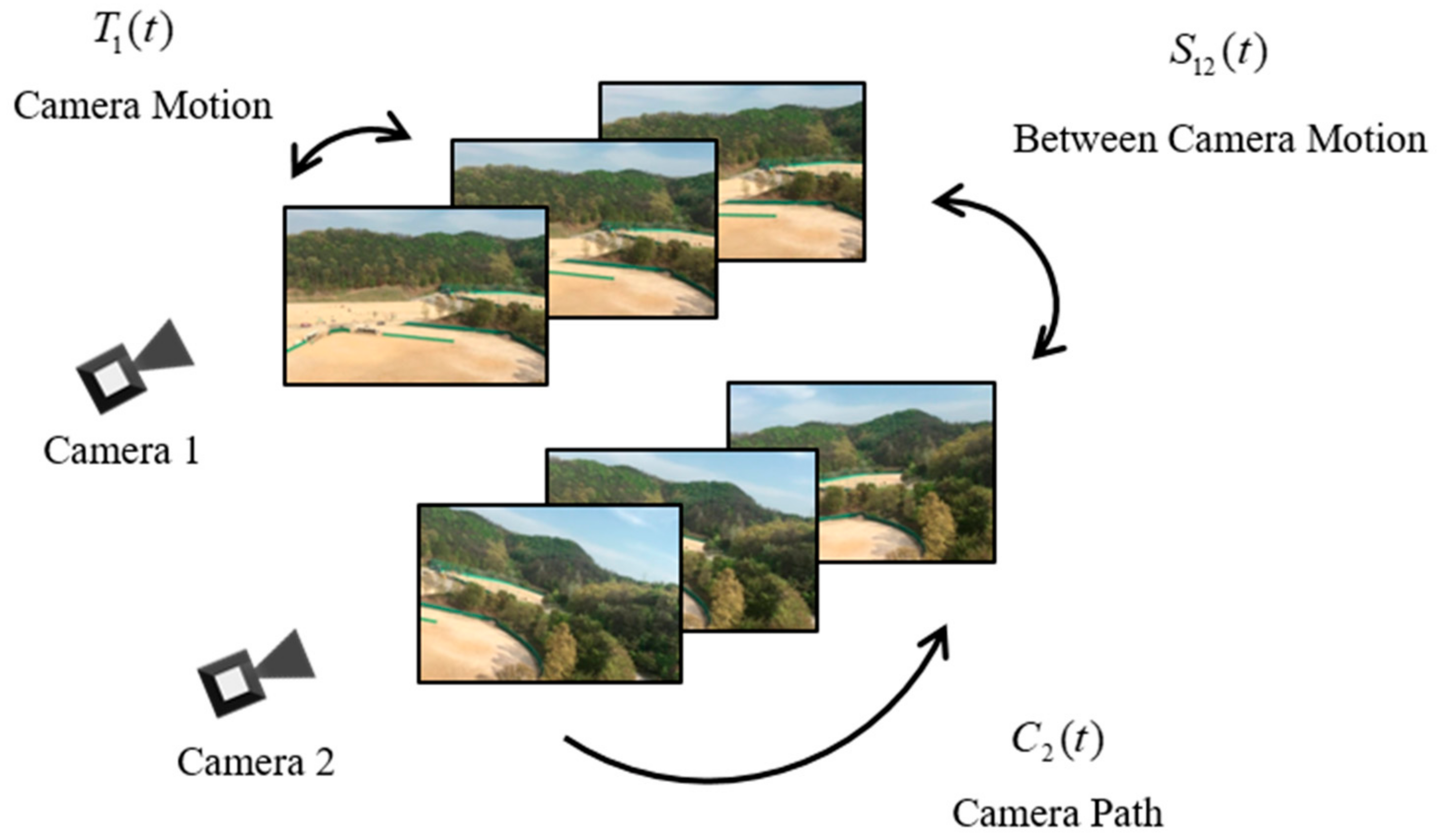
In this section, we introduce various motion models to understand our frameworks easily. The motion model is a numerical representation of camera movements between two images. In the stitching algorithm, the homographies are used to obtain the motion models. The process of video stitching needs two type of motion models, which are spatial motion model and temporal motion model, unlike an image stitching algorithm, which in principle needs only a spatial motion model. The spatial motion models are BC homographies that represent the homographies between the multiple inputs in the same frame. is the BC mapped from camera to in the frame . The temporal motion models consist of successive CMs and CPs. The CMs are the homographies between neighboring frames of the same cameras. is the CM of camera between the frame and . The CP is accumulated by the individual CMs. The CPs are important components for accurate video stitching. In the Section 3.2, this process is discussed in detail. The CP is denoted as for the camera at the frame . It can be written as
where {} are the products of the CMs. Figure 2 shows the BCs, CMs, and CPs.
3.2. Basic Theory
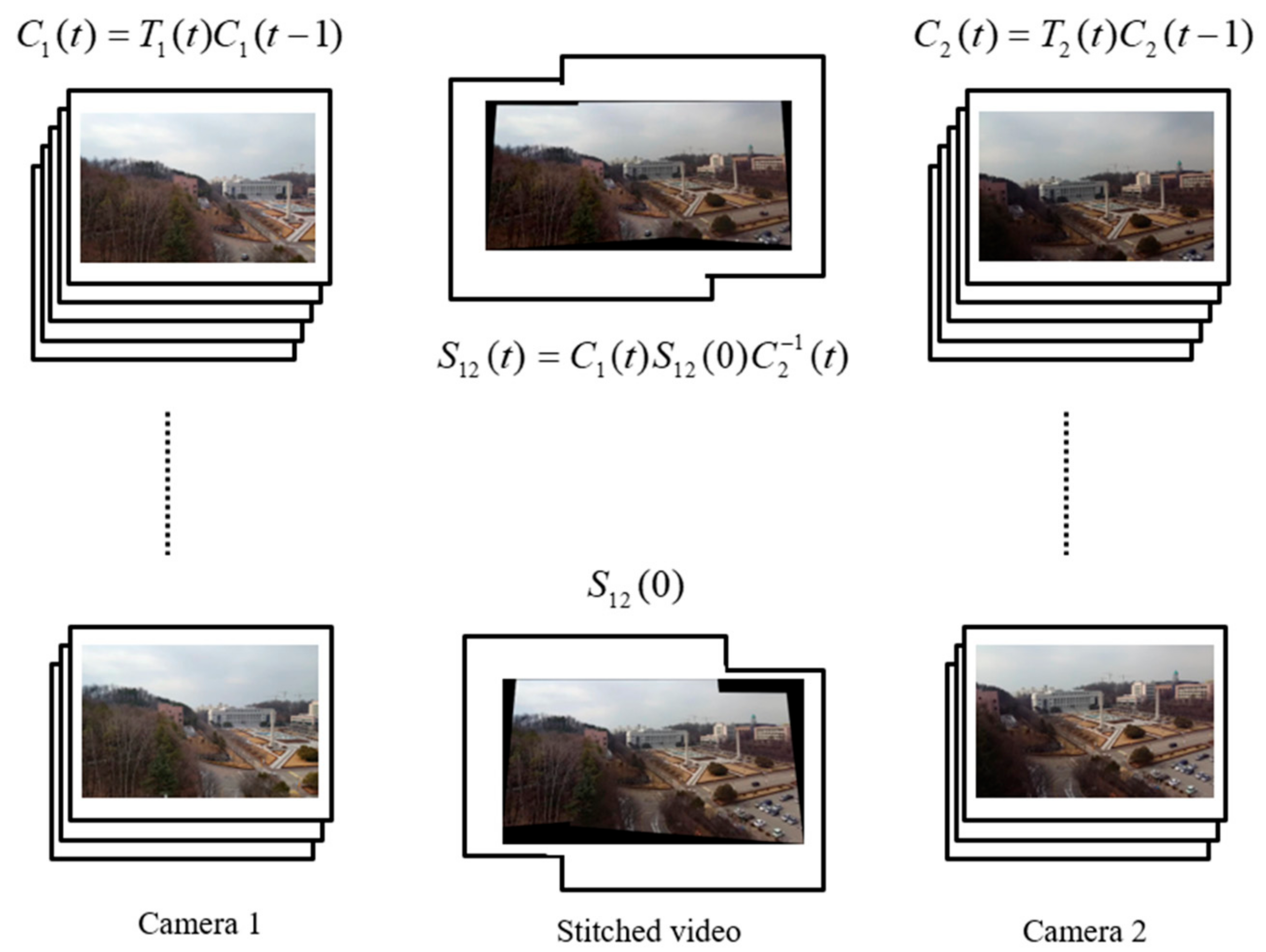
In this section, we introduce a theory based on the proposed method. Video stitching is implemented using the BCs and CPs. Therefore, the relationship between the CP and BC should be understood. Figure 3 shows the relationship between the CP and BC. The CP is a product of the CMs, as expressed in (1). The BC is
where and are the CP at the cameras 1 and 2, respectively. is the initial BC of the first frame. can transform the coordinates of the frame at the camera 2 on the basis of the coordinates of images captured from the camera 1.
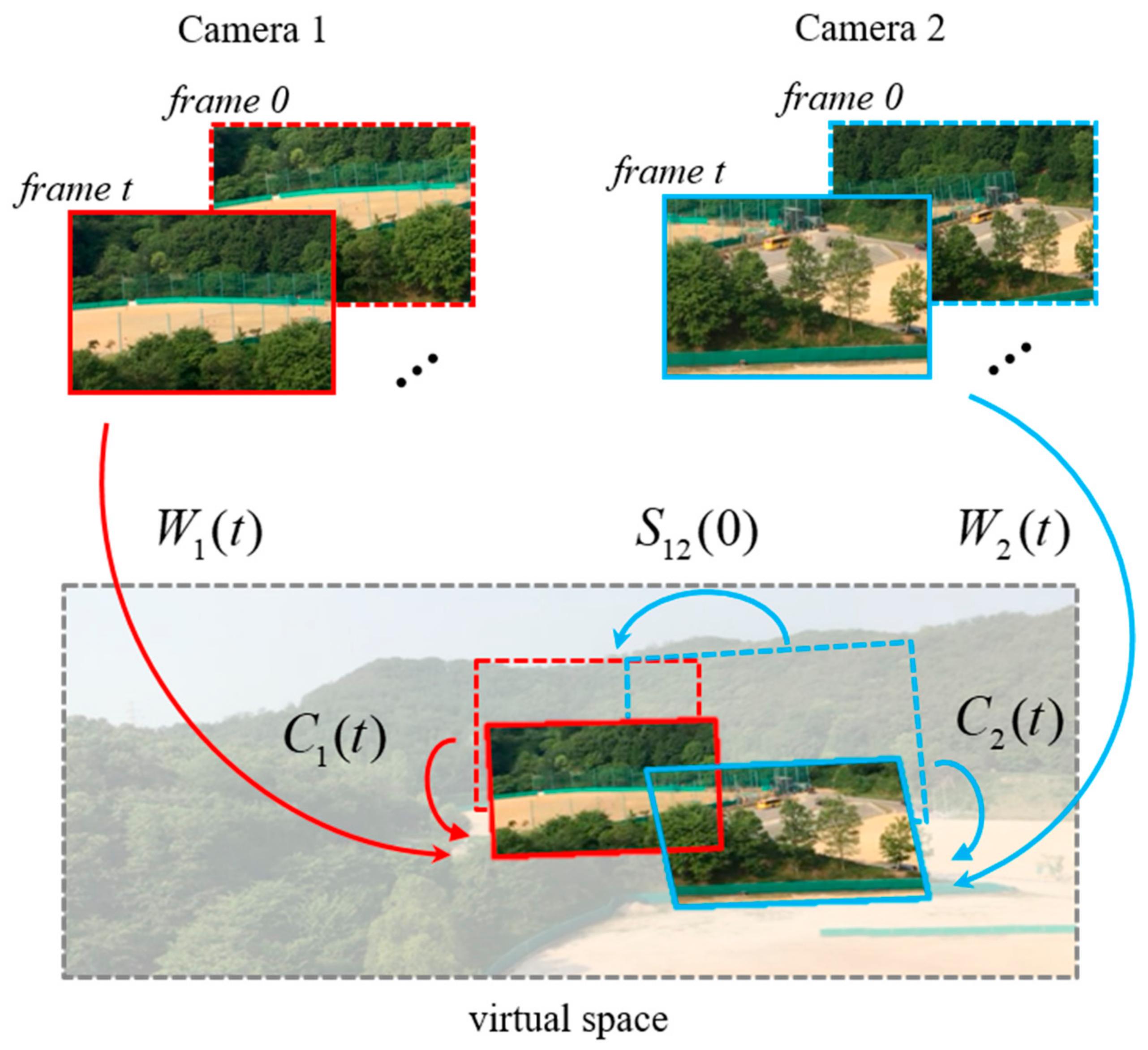
However, the BC is not used for a transformation of the coordinates between the frames. Because the references of frames are changed dramatically, the motion of the transformed frames may become more dramatic. Thus, the reference is set as the first frame for obtaining the stable results that seem to be taken with a fixed camera. For this work, we need warping motions (WMs) that transform the matrixes for mapping from the frames to the reference of the first frame. We denote WM as , with camera at the frame . The WMs are composed of the CPs and the initial BC. Figure 4 demonstrates the relationship among the WMs, CPs, and BCs. In the top of Figure 4, the red boxes are the inputs of the camera 1, and the blue boxes are the inputs of camera 2. Boxes with a dotted line are the inputs at the first frame, and boxes with a solid line are the inputs for individual frames denoted by . In the bottom of Figure 4, each input is transformed by the WM on the basis of the first frame of camera 1. The equation representing the WM can be written as
where and are the WMs of the cameras 1 and 2, respectively, and are the CPs, and is the initial BC between camera 1 and 2 at the first frame. Note that (3), (4) are valid when the CPs are accurately estimated.
3.3. Proposed Method
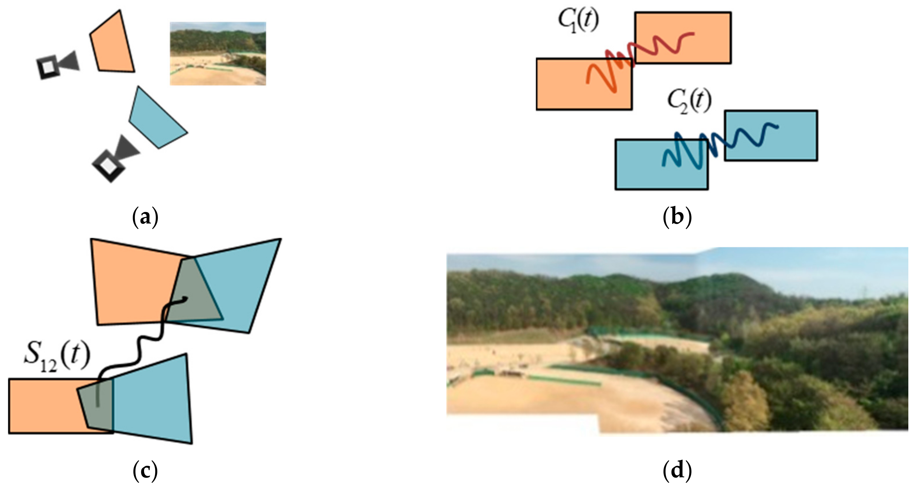
Our framework has four stages. Figure 5 shows the flowchart of our framework. The first step of our algorithm is to obtain inputs from the multiple moving cameras that have a certain degree of freedom (swing, shaking, etc.). We enforce a rough synchronization by initializing recording of the scenes at the same time.
The second step is to estimate the CPs. The proposed method differs from the existing estimation methods. The existing methods use SIFT and SURF for feature extraction, and FLANN for matching features. This approach is not appropriate for a real-time video stitching algorithm, due to the excessive processing time requirements. Therefore, we propose a novel method of CP estimation to reduce the processing times. Our method extracts the features in every frame using the intensities of frames on the grids, and makes matching points by tracking the features using the optical flow method.
The third step is to refine the BCs. The misalignments sometimes are observed in the results as a result of inaccurate CPs. To remove the misalignments, we repetitively estimate the error motions using block matching. Then, the inverses of the error motions are multiplied to the current BC.
The final step performs the warping and blending. For the warping stage, we estimate the WMs using the CPs and BCs and generate the warping images by multiplying WMs to the frames. At the blending stage, we remove the visual seams that are generated by the intensity differences between the two images. In our framework, a multi-band blending [26,27] is adopted as the blending method.
4. Camera Path Estimation
In this section, we introduce the details relating to the CP estimation process. For a real-time system, the fast homography estimation method is required. On a PC with Intel i5-4590 3.4GHz CPU, the existing methods using SIFT and FLANN require 2–3 s of CPU time to generate a high-dimensional descriptor of the features. However, this paper proposes a fast CP estimation method without the use of descriptors. The proposed method measured 0.01 s on the same experimental environments. It means that the proposed method is more suitable for real-time systems.
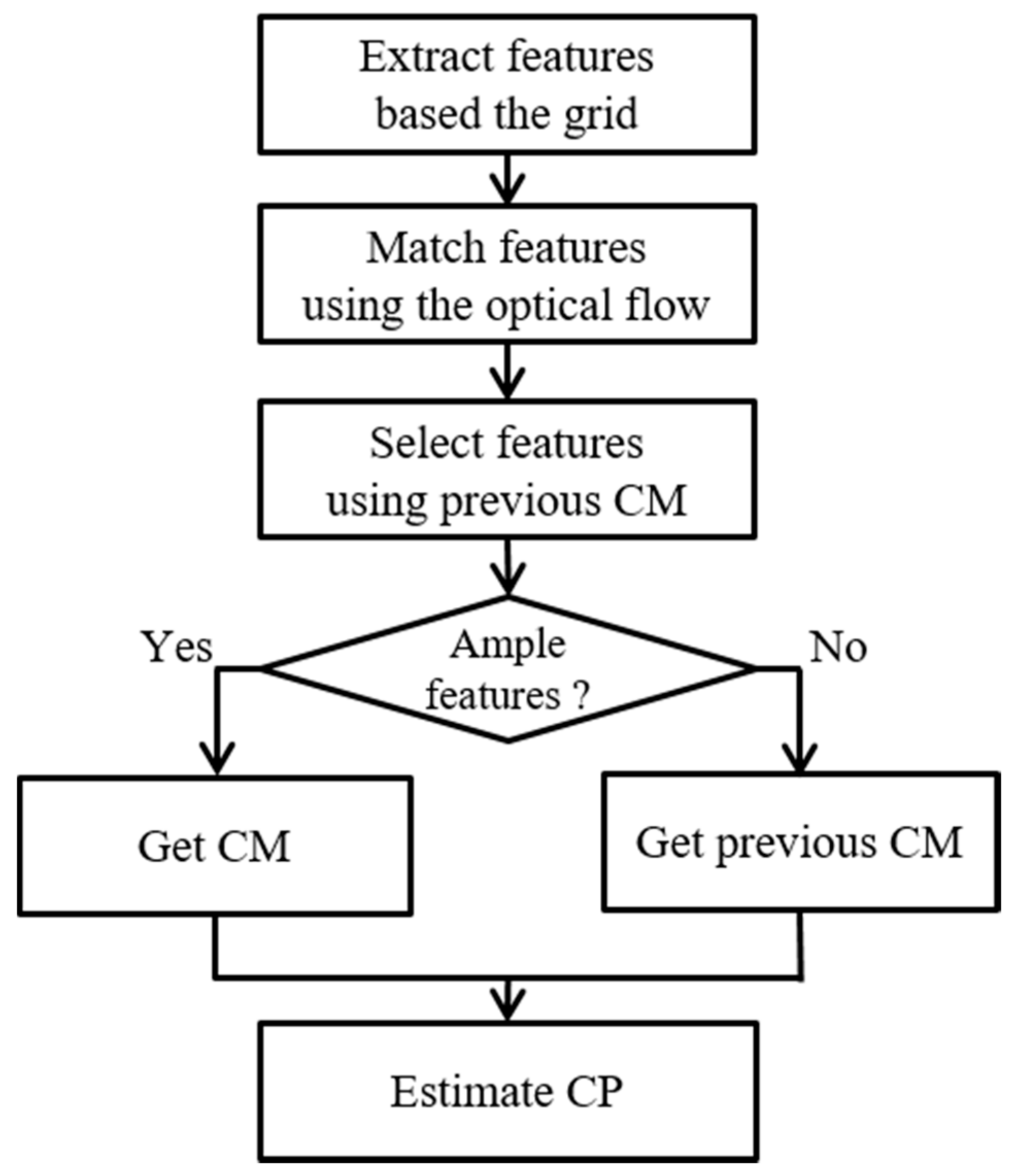
The proposed CP estimation method largely contributes to the field for two reasons: (1) the uniform features extraction, and (2) the fast feature matching. The first method is uniform feature extraction based the grid. The CP estimation is sensitively affected by the distribution of features. For example, assume that the features are densely gathered on the certain region; the features then create a local homography, instead of a global homography. This local homography produces results that include the misaligned artifacts. Therefore, the features should be distributed uniformly. For the uniform distribution, the features are extracted using the grid. The second contribution of this approach is the fast feature matching using the optical flows. Traditionally, when matching features, calculating the descriptors takes a long processing time. Therefore, we need to define a new feature matching method without the descriptors. In the method, the matching points are obtained by tracking the features using optical flows. Figure 6 shows the flowcharts of the CP estimation method.
4.1. Feature Extraction
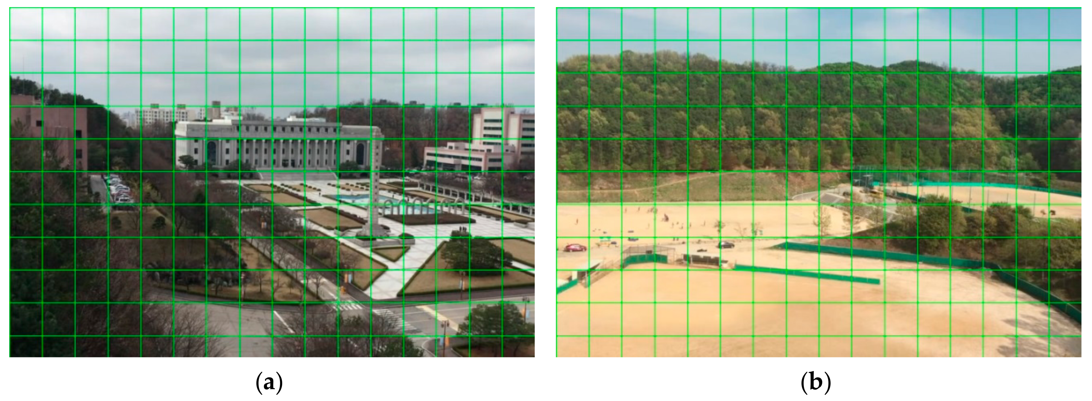
The feature extraction process, based on the grid, is made up of two steps: (1) frame division for a uniform distribution of features, and (2) feature extraction using the intensity of difference between adjacent frames. First, we divide the frames of input into a grid. Figure 7 show the inputs which are divided into a grid. The green lines are the lines of grid. The grid size is empirically set to 70 at the HD resolution (1280 × 720 pixels). The vertexes of a grid become potential features for extracting the features. After dividing an image into a grid, we select the features in the candidates on the vertexes of the grid. Second, the extraction method uses the difference of the intensity between the current and previous frames:
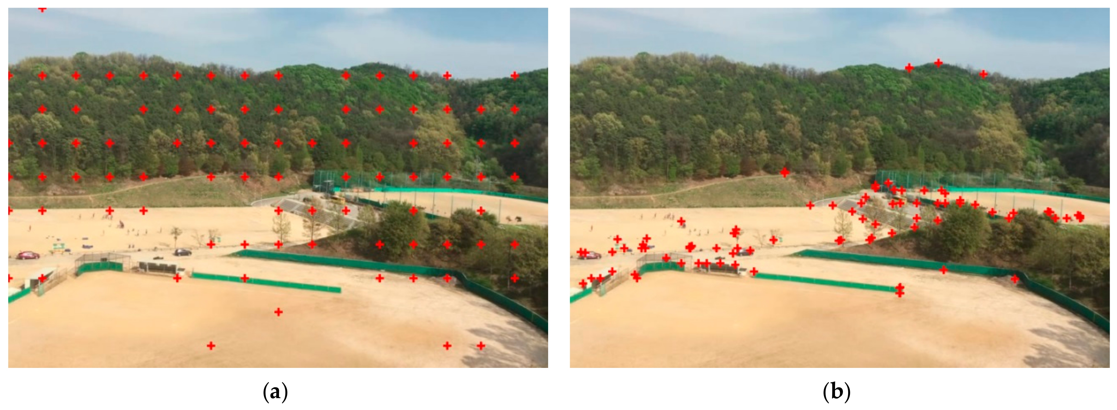
where and are the coordinates on the vertexes of the grid, and are the intensities at the current time and previous time , respectively, and is a threshold (we use ). Figure 8a shows the features by using (5).
The feature extraction based on the grid is not only fast, but also stable. Our extraction method produces a more stable CM than the other methods. For example, when applying the general method into the frame, such as with Harris corner detection [28], we frequently confirm that the features are densely located in certain regions, as shown in Figure 8b, because the method produces more features on the highly textured regions (e.g., the buildings, the trees) than the poorly textured regions (e.g., the sky, the roads). The biased feature distribution estimates the local homography based on the planes with the greatest number of features. Estimating the CM using the local homography, we obtain poor results that are concentrated on a plane with many features. In contrast, our proposed method extracts the uniform features. This approach estimates a global homography which produces better results than any individual local homography.
4.2. Feature Matching
In the traditional stitching method, the matching methods use the features including the high-dimensional descriptors. For making descriptors, the matching algorithm performs a complicated process. This method needs much more time to obtain a result. Therefore, we need new feature matching methods, without the use of descriptors.
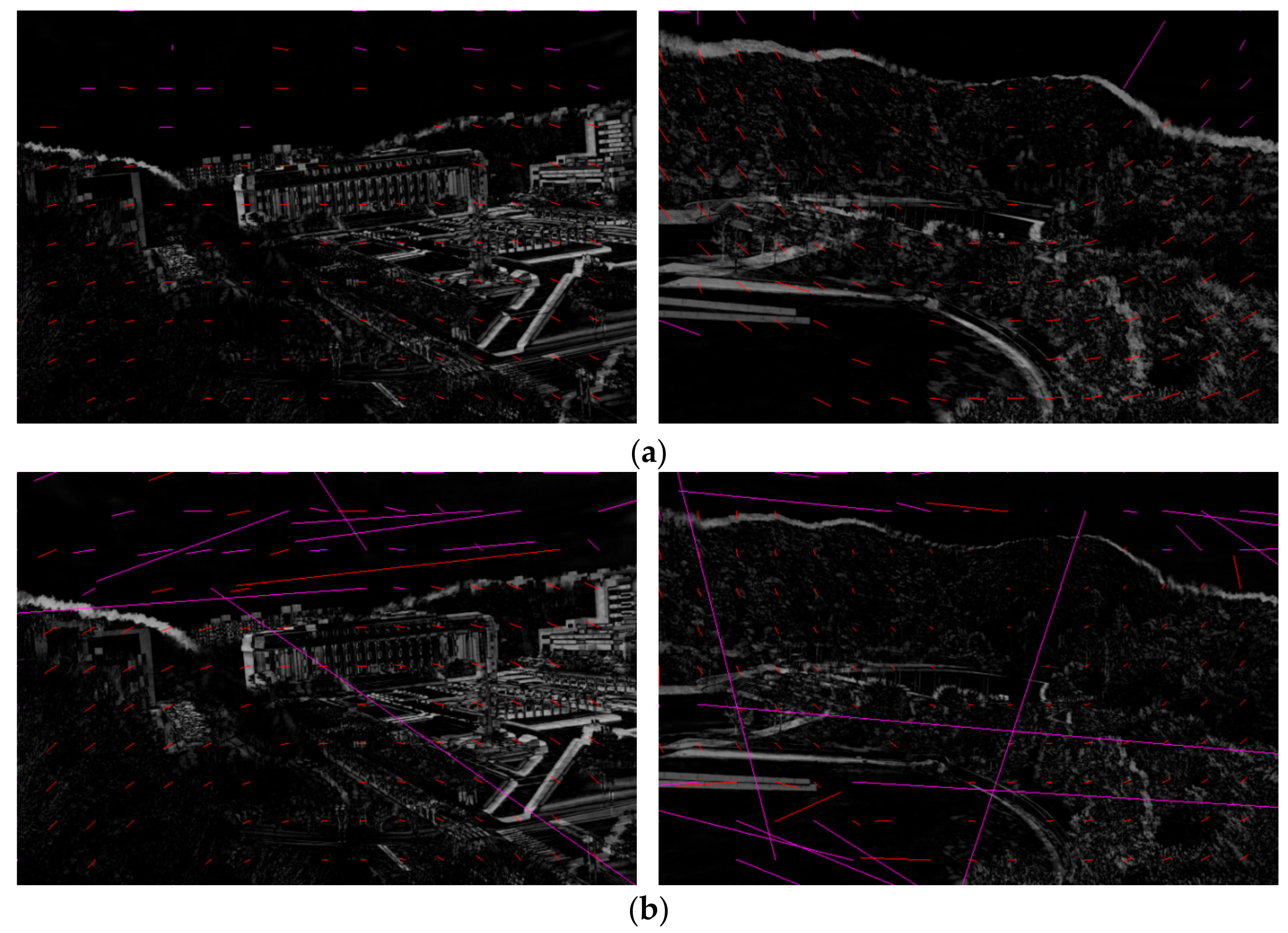
For fast matching methods without the descriptors, we use the optical flow method. The optical flow method is a tracking algorithm that aims to find target objects between neighboring frames. The purpose of the optical flow method is to track objects. However, we use optical flow for tracking the features, instead of the objects. We use the positions of features as the seeds for the optical flow, and track the features. Figure 9a shows the tracked features using the optical of the images with difference of intensity between the previous and current frames. The red lines are the well-tracked features.
The tracking errors may be observed due to the similar patterns of the regions between the current and previous frames. To remove the tracking errors, we use the following equation in the [12]:
where is the L1 distance between initial points and tracked points , is the number of pixels in a search window, and is a threshold to determine whether the point is correct or not (we use ). By using constraint (6), the tracking errors are removed, as shown in Figure 9b.
4.3. Feature Selection
In this section, we describe the feature selection method. In general, the feature distributions of the frames are similar, because the difference in time between the frames is very small. However, different feature distributions often appear due to changes in illumination or dramatic movements of the camera. This fact often makes for the unstable results. To guard against these situations, we implement a feature selection process before estimating the CM.
The feature selection protects against two unwanted situations: (1) different distributions of features are compared with the previous frame, and (2) no feature points are identified. First, the distribution of features is sometimes different from that of the previous frame. This situation produces the discontinuous result. For solving this problem, it is supposed that there is little difference between the current and previous CMs. Using this supposition, we transform the current features using the previous CM. Then, we calculate the Euclidean distances between the features transformed by the previous CM and the features tracked using the optical flow method. The distance is checked for whether it is smaller than a threshold. The features with distances smaller than a threshold are regarded as the inliers. Finally, the CMs are estimated by the inliers using RANSAC, and are multiplied by the previous CP to estimate the new CP. The method is defined as
where is the L2 distance between features transformed by the previous CM and the tracked features using the optical flow. is the threshold. We set this threshold to . Then, the CMs are estimated by the inliers using RANSAC, and are multiplied by the previous CP to estimate the new CP.
Second, we prevent the case that extracts the small amounts of inliers after selecting the features. If the CM is estimated using a small number of features, a wrong CM may be estimated. To prevent this undesirable situation, we adopt a simple method that replaces the current CM with the previous CM. This method can be exploited because there is little difference between the adjacent CMs.
5. Homography Refinement
In this section, we describe how to refine the BCs. In the process of video stitching, the coordinates of different cameras are represented on the common space using Equations (2)–(4). However, the BC can include the errors resulting from inaccurate CPs, which are estimated incorrectly due to dramatic camera movement or intensity changes. Therefore, we propose to accomplish BC refinement by using block matching.
When the observation of BC is defined as
where and are the observation of CPs that includes the error motion , the relationship equation between the observation of BC and the ideal BC is estimated as
Actually, the error motions between the adjacent frames have little effect on the misalignments. However, the errors are accumulated over time. At the last frame, the results include remarkably misaligned artifacts. This will be illustrated in Section 6. Therefore, observation of the BC must be updated by multiplication with the inverse of as follows:
where is the refined BC. In practice, the refined WMs and are estimated using (11) to warp the images:
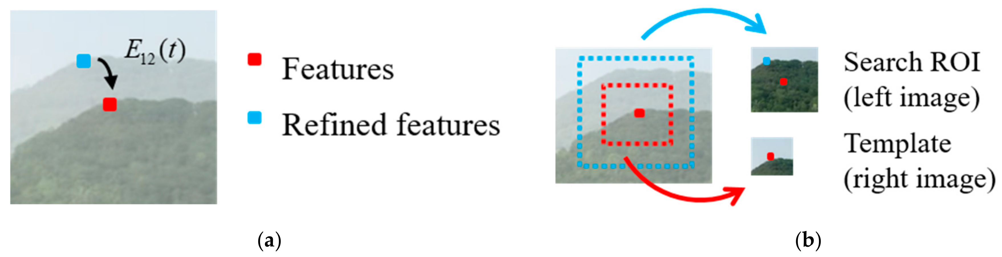
To update the refined BCs, the error motion should be estimated using the features and the refined features, which are the ideal features for stitching, as shown in Figure 10a. In other words, the locations of the refined features are found. The simplest method for finding the refined features is the method using SIFT and FLANN. However, this method is not suitable for a real-time system, due to the long processing time. Therefore, we estimate the error motion using block matching. The block matching is a matching algorithm that finds locations of templates. To find refined features, a template is constructed around the features from the right frame and a search ROI, which is the search range for block matching, and is built on the left frame, as shown in Figure 10b. Then, the error motion is estimated by implementing the block matching algorithms.
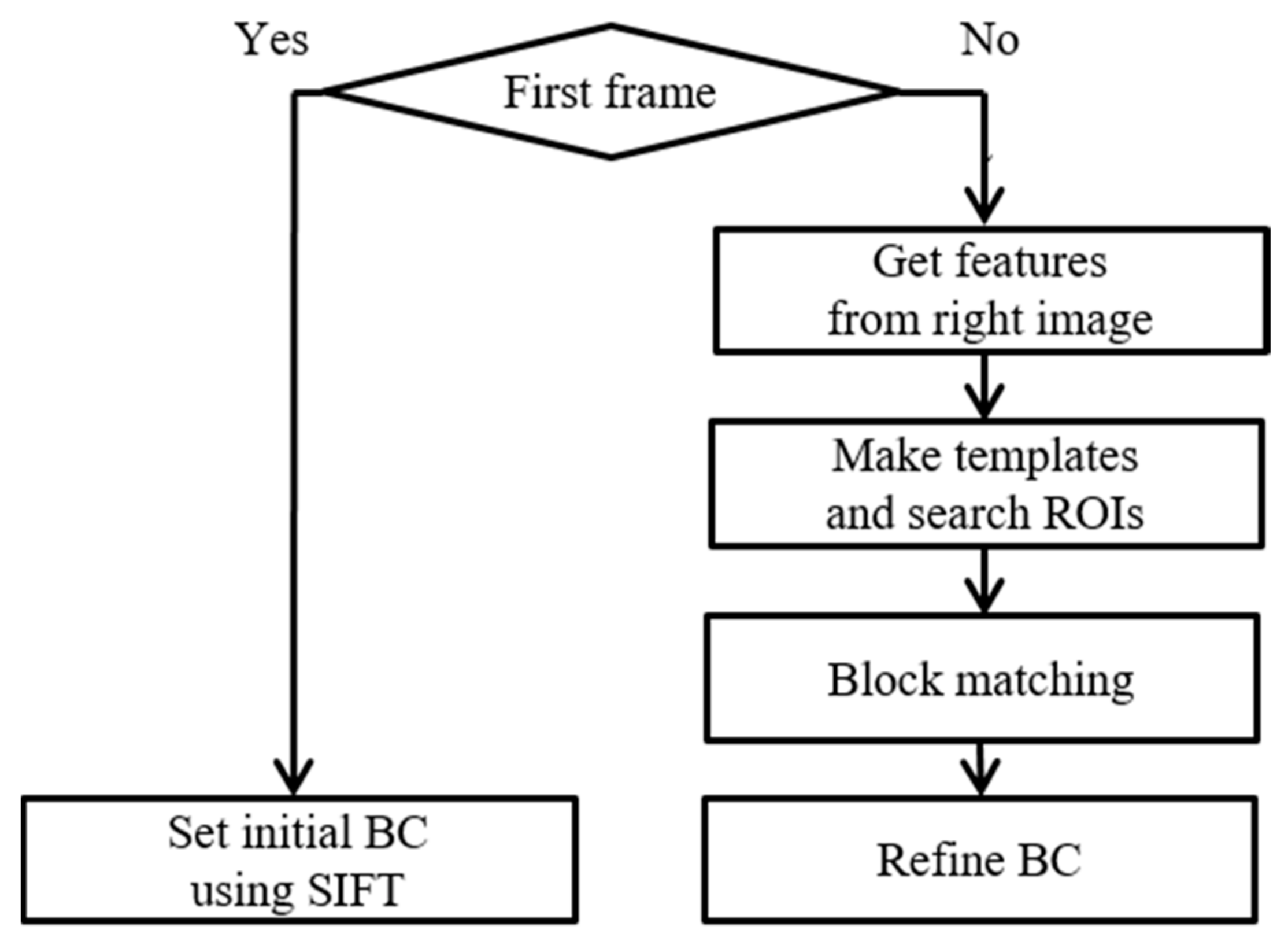
Figure 11 shows the flowchart of the homography refinement in detail. In the first step, we calculate the initial BC by using SIFT and FLANN at the first frame. Though this initial step has a long processing time, it is important to accurately estimate the initial BC, which is used as a reference for the refined BCs. In the second step, we reuse the features, which are obtained in the CP estimation, from the right frames, to construct the templates and search ROIs. In the third step, we form the templates of size ( × ) and search ROIs of size ( × ) around the warped features in the warped right and left frames, respectively. We define , as 9, 21, respectively. In the fourth step, we carry out the block matching to estimate the error motions. The block matching uses the normalized cross correlations (NCC) to measure the matching rate between the templates and search ROIs:
where and are pixel coordinates in the warped frames, and are pixel coordinates in the templates, is the value of NCC, and are the intensities in the warped frame and templates, respectively. We select the features with a maximum as the refined features. Finally, the current BCs are updated by the error motions, which are estimated by the refined matching points using the RANSAC algorithm and using (11).
6. Experimental Results
To evaluate the performance of the proposed method, we performed three experiments as follows: (1) we evaluated the performance of our method using a variety of samples (i.e., processing time and stitching qualities), (2) we demonstrated the performance of this CP estimation and homography refinement approach by comparing it with other methods, and (3) we found the optimal parameters.
We tested our method on a PC with an Intel i5-4590 3.4GHz CPU and 4G RAM. Our method is implemented using C++.
Input videos used in the experiments are acquired by the iPhone 6s with a resolution of 1280 × 720 pixels at 24 fps.
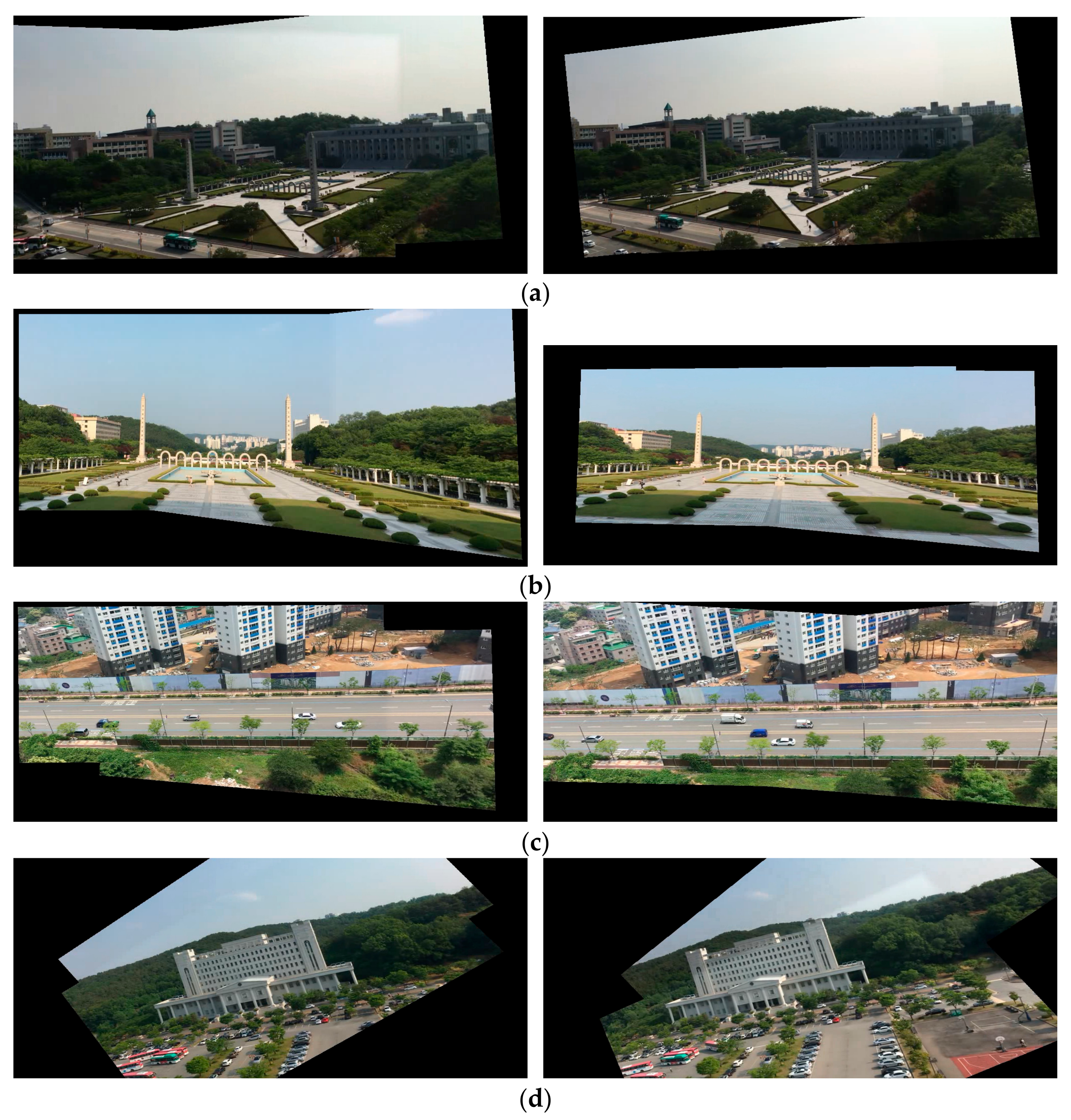
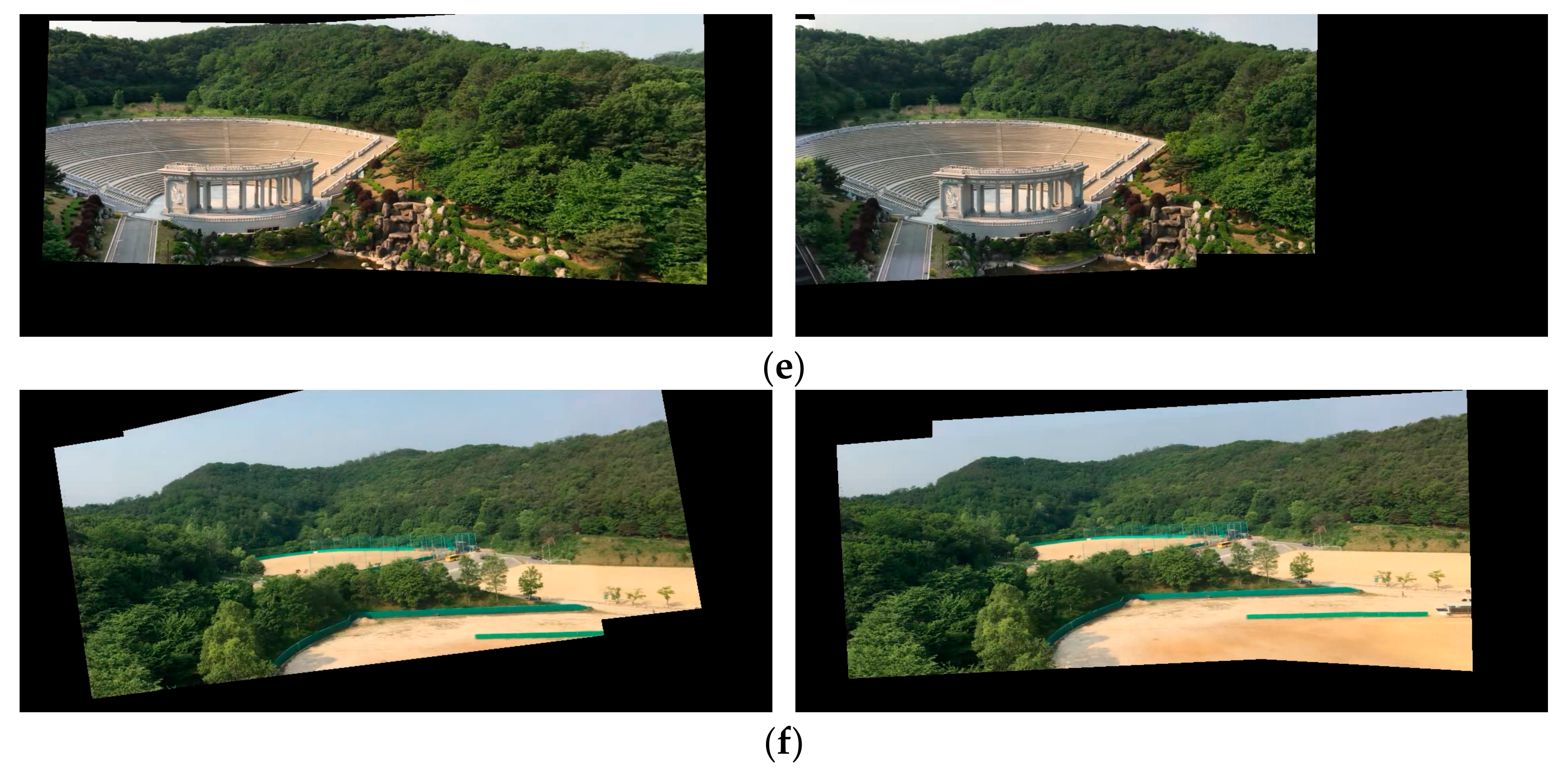
To validate our method, we collected various kinds of video samples, with six of these shown in Figure 12. Here, the samples include diverse environments (streets, building, etc.) and many kinds of camera motions (swings, parallel translations, dynamic moving). The first, second and third examples contain various environments. The third example contains a moving object. The fourth, fifth, and sixth samples are filmed under various camera movements, i.e., swings, parallel translations, and dynamic moving, respectively (the original videos and experimental results can be found at [29]).
6.1. Processing Time and Stitching Quality
The important components, which indicate the performances of the video stitching, are the processing times and qualities of alignments. To show the two performances, we measured the processing times using the win32 API and the stitching score proposed in [6], using samples 1–6, as shown in Figure 12.
Table 1 shows the processing times using the six samples. On average, the proposed method spent 11.0 ms, 6.2 ms, 15.6 ms, 42.0 ms, for the camera path estimation, homography refinement, warp and blending, respectively. The total processing time is 75.6 ms (i.e., about 13.2 fps). In Figure 13, it is demonstrated that this method takes less time than video stitching using SIFT, which takes about 3.9 s. The proposed method approximately shortens the processing time by a factor of 50. This confirms that the proposed method is suitable for real-time systems.
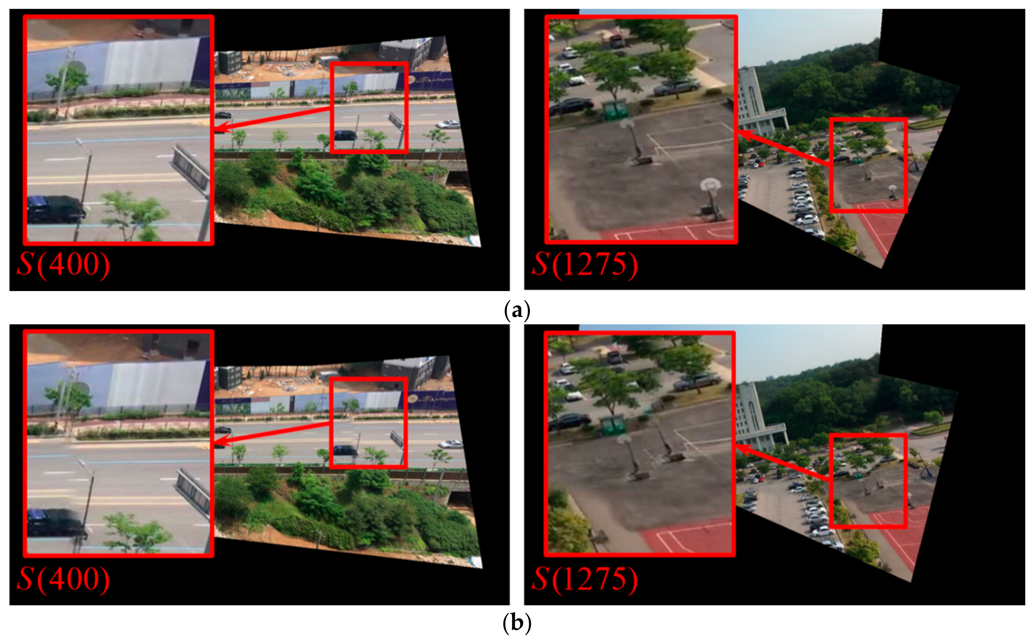
Now, we evaluate the alignment quality. For numerical evaluation of the alignment quality, the stitching scores, which are proposed in [6], are measured. To explain briefly, the stitching score is the L2 distance between features transformed in the estimated homography and ideal homography. For the ideal homography, we re-estimate the new homography between two frames using SIFT and FLANN. The new homography is considered as the ideal homography. A smaller stitching score represents a better quality of alignments. Table 2 shows the stitching scores that compare the two cases with and without homography refinement, using samples 1–6. In Table 2, the average stitching score without the homography refinement is 6.433. When applying the homography refinement, the average stitching score is 1.027. We numerically confirm that the homography refinement removes the error motion caused by the accumulated errors, as shown in Figure 14.
6.2. Comparison with Other Methods
To reduce the processing time, we tried a variety of methods. In particular, we strived to improve the features extraction process in CP estimation, and improved the process of finding the refined features in the homography refinement. In the feature extraction process, we experimented with the proposed method, good feature to track (GFTT) [30], and Harris corner detection. In the matching methods, we ran experiments with the proposed method and nearest neighbor search (NNS). The stitching score and processing time are shown in Table 3 and Table 4. In Table 3, we measure the stitching score without homography refinement and processing time during the CP estimation process. In the Table 4, we measure the stitching score with homography refinement and the processing time during the homography refinement. The results are obtained based on the first sample in Figure 12.
GFTT and Harris corner detection were used as feature extraction methods in CP estimation, and were compared with the proposed method. First, GFTT is also a feature extraction algorithm for the tracking algorithm. Features obtained using GFTT are uniformly dispersed. Due to suitable feature detection for tracking objects, GFTT has a better stitching score than the proposed method. However, GFTT has the notable disadvantage of a greater processing time. Second, Harris corner detection is a basic detection algorithm using the Hessian matrix. Although the stitching score of Harris corner detection is equal to that of the proposed method, the processing time incurred by the Harris corner detection is five times larger than that of the proposed method. Additionally, Harris corner detection has the disadvantage that the local CMs are estimated, as shown in the Figure 8b.
To illustrate our superior performance of finding the refined features, our method is compared with NNS. NNS is a simple matching algorithm that selects the closest features. Below, we present the instructions of NNS for matching features. We first establish the ROI around the features. The matching candidates are regenerated using the feature extraction in the ROI. The nearest candidate from features is selected as the matching points. The NNS requires less processing time than the proposed method. For the stitching score, however, the NNS algorithm is woefully inadequate, because the method only uses the distance information. Thus, NNS is inappropriate for matching algorithms.
6.3. Parameter Optimization
We will define appropriate parameters for our system. Our system uses various parameters in both the CP estimation and homography refinement. Among various parameters, this section is focused on six parameters that are mentioned above. The six parameters can be categorized into two types of the parameter: (1) size type (i.e., the size of the grid in the CP estimation, and the size of templates and search ROI in the homography refinement); (2) threshold type (i.e., , , and ). The six parameters are optimized by the experiments. To optimize the type of size, we measured the processing times and stitching score with changes in the value of the parameters, because the type of size influences the trade-off between computational complexities and quality of stitching. Similarly, the threshold types are optimized by comparing the results of tests with change in the threshold values.
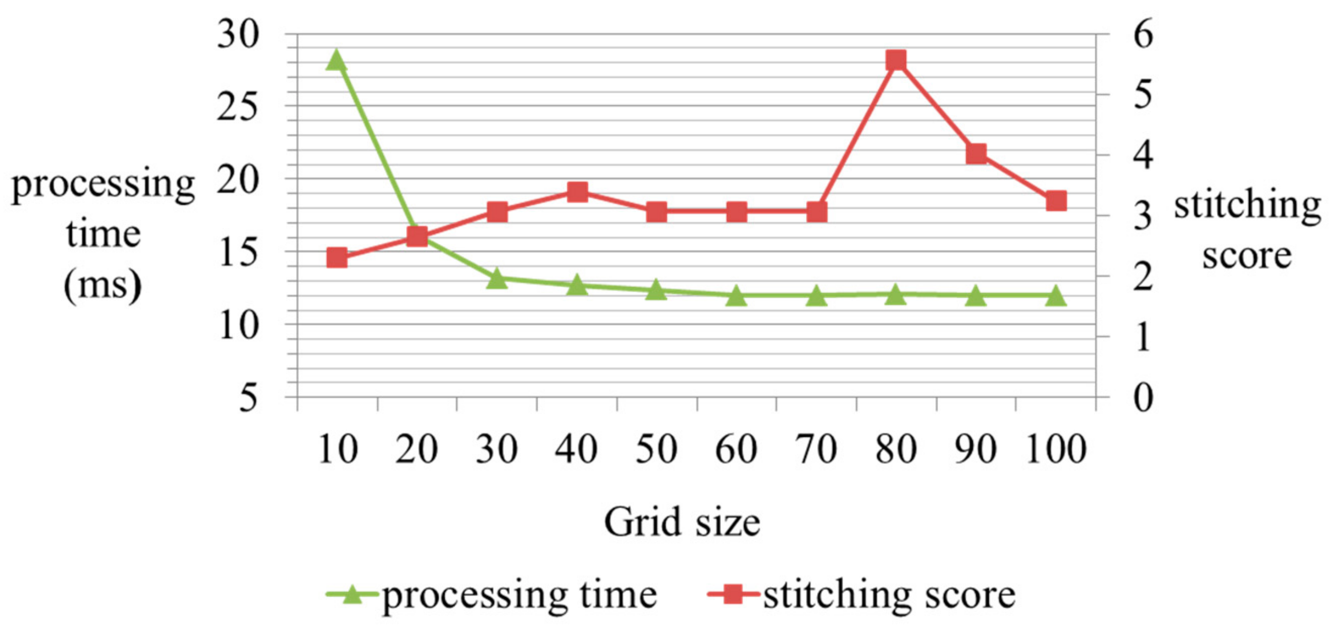
The size of the grid influences the number of features. The smaller the grid size, the more features are extracted. Figure 15 shows the stitching scores and processing times as a function of the changes in the grid size. We first measure processing time in the CP estimation step. We then calculate stitching scores without the homography refinement. In Figure 15, the processing time generally decreases by increasing the grid size. In detail, the grid sizes with 30 or more elements show no change in processing time. However, the stitching score is independent of the grid size, while a large grid size has a higher probability of leading to misalignments. On the whole, a high score is observed with large grid size. At the grid size of 80 elements, the highest score is obtained. Therefore, we consider the results of experiments to maintain a balance between the processing time and the stitching score. In this framework, we select grid sizes of 70 elements.
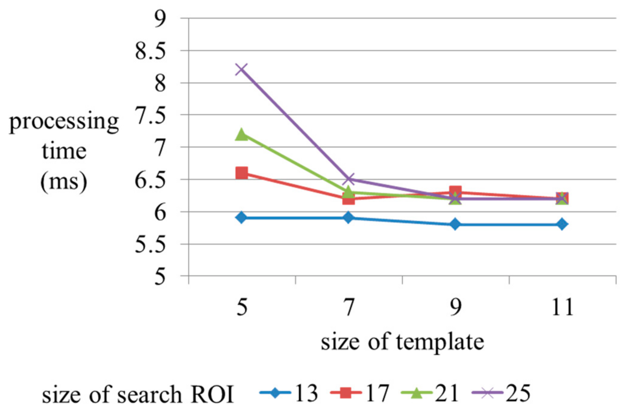
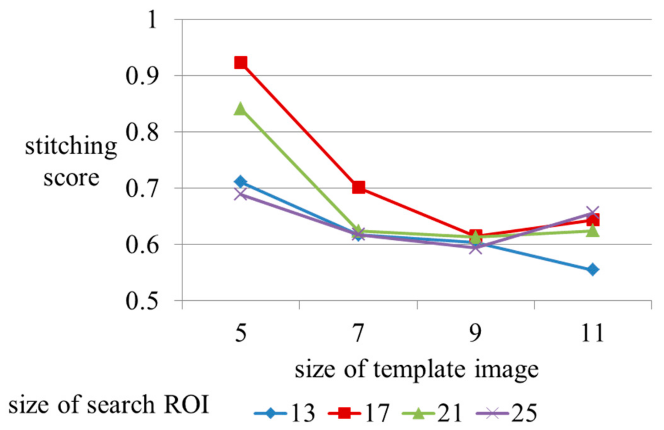
In the block matching process, the size of the template images and search ROI are important parameters relating to the computational complexities. Figure 16 and Figure 17 show the stitching scores and processing times as a function of changes in size of the template and the search ROI. We measure processing time during the homography refinement step. We calculate stitching scores after completion of the homography refinement. In Figure 16 and Figure 17, we confirm that the stitching score and the processing time gradually decrease with expansion of the template image, and are unrelated to the size of the search ROI. Figure 16 shows that the size of the template has little impact on the processing time, except for a size of 5. According to the results, we only consider the size of the template for the optimal parameter. But the large size of the search ROI is an important component. Inputs with fast movement require a wide search range. If a small size is set for the search ROI, inputs with fast camera movement are inappropriate for consideration. Therefore, we should consider an optimal search ROI. In the paper, we set the size of the template image and search ROI as 9 and 21.
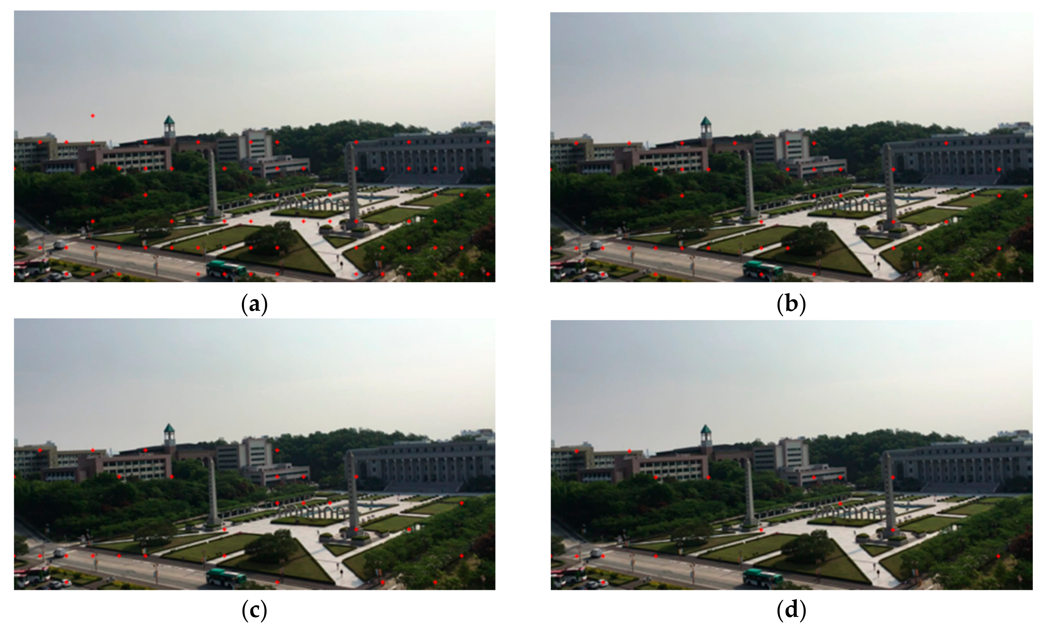
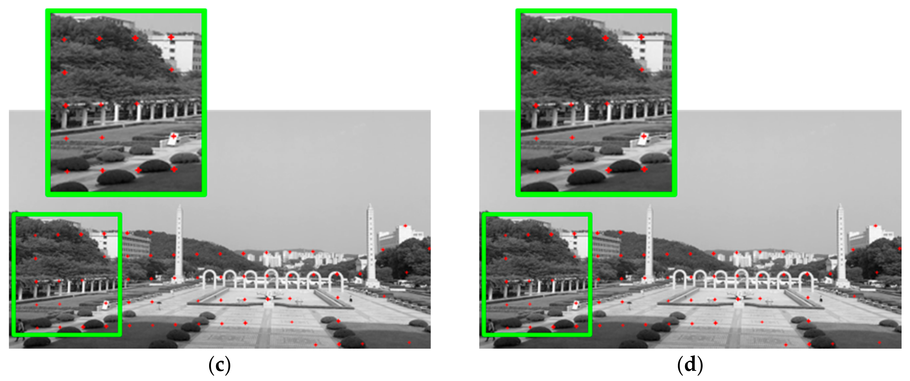
To set the appropriate value of threshold in the (5), both the number and position of features are considered. Figure 18 shows the results of experiments with a change in value of the threshold. The red crosses indicate the positions of the features. In the Figure 18a, some features are extracted on the poorly textured region like sky, causing the errors of optical flow. In the Figure 18c,d, although the features are extracted on the highly textured region, the number of features is insufficient for homography estimation. Therefore, an optimal threshold value is set to 5.
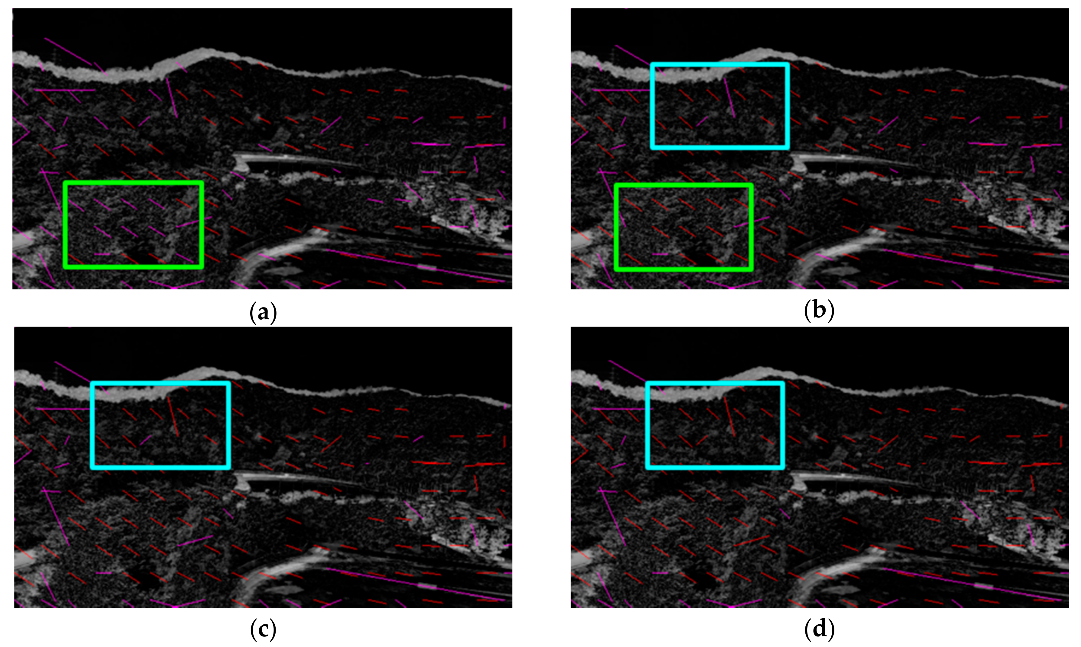
The value of threshold in (6) is also optimized by comparing the results of experiments. The role of threshold is to distinguish errors from the feature tracking. Therefore, when the optimal is set in (6), incorrect flows are classified as the false detection. Figure 19 is the results of experiments with change in the value of . Red lines indicate well-tracked features, and magenta lines indicate the errors. In the Figure 19a, the well-tracked features are recognized as the errors in a green box, unlike a green box in the Figure 19b. On the other hand, in the Figure 19c,d, the errors are missed in a cyan box. According to the results, the value of is set to 5.
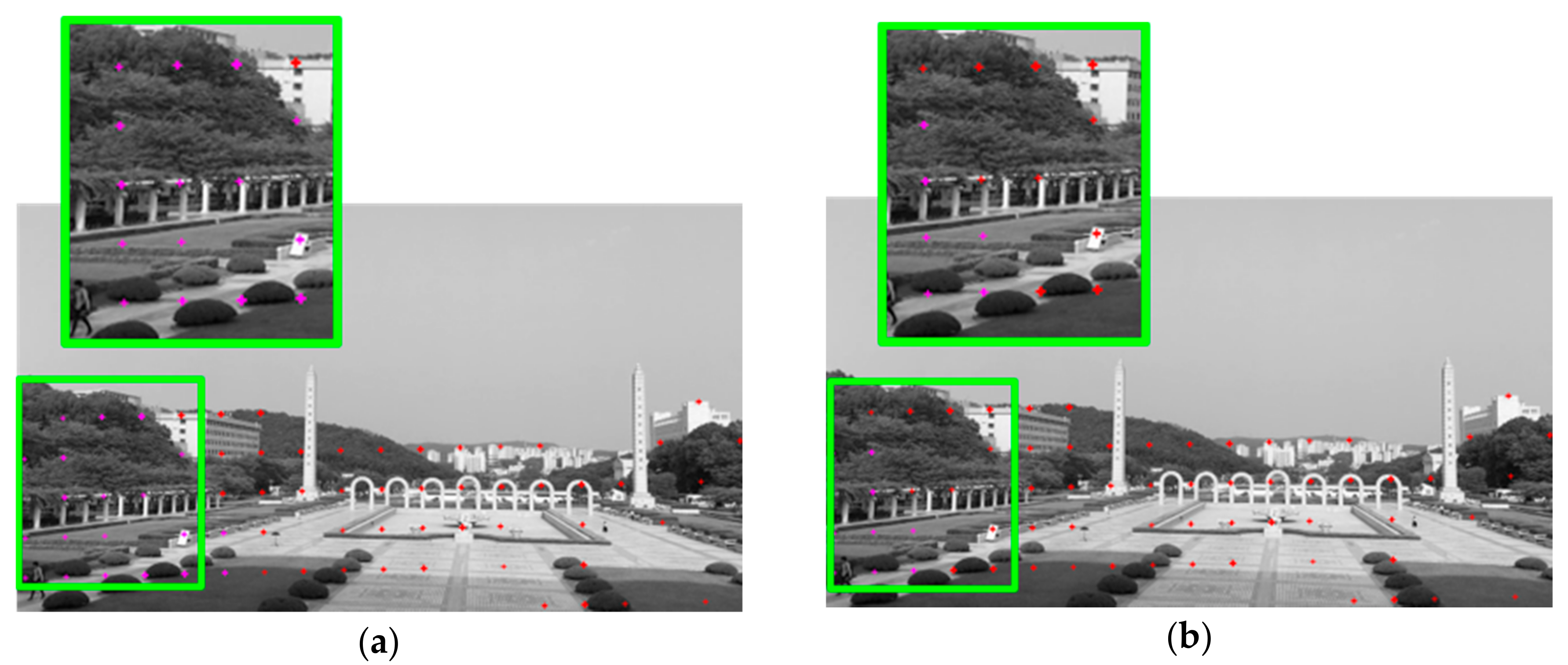
Finally, we estimate the threshold value to analysis the results of experiments with change in value of . In the Figure 20, we can compare with the results using (7) in the green boxes. The red crosses indicate the selected features, and the magenta crosses indicate the unselected features that are insufficient to be selected for estimation of homography. In the Figure 20c,d, the selected features are over-selected, while the proper features are selected as shown in Figure 20a. Therefore, in the paper, the threshold is set to 30. However, it notes that the can be adaptively set according to movement of the cameras. In the case that the movement of cameras is dynamic, is set to a higher value than the optimal value of 30.
7. Discussion
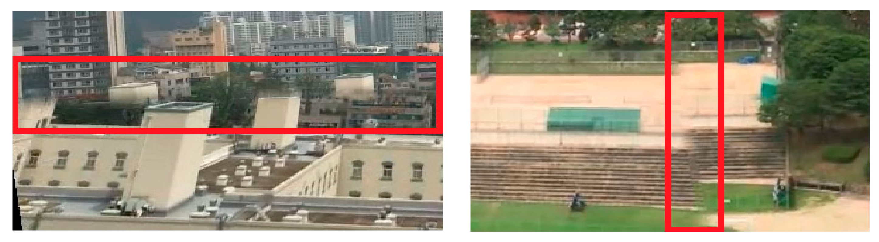
In this section, we describe limitations. Although our method demonstrates an improvement over previous work, samples of failure are sometimes observed, as shown in Figure 21. By analyzing the samples of failure, we determine that they occur due to two reasons: (1) a dramatic movement of camera, and (2) multiple planes in the scene. The first reason, a dramatic movement of camera, produces weird and unusual CPs. We suppose that videos must have continuity between adjacent frames for the optical flow. However, a video with a dramatic movement may have discontinuities that are susceptible to producing errors. Moreover, under these conditions, the template images cannot be matched in the homography refinement, because the variation of scenes is beyond the range of the search ROI. The second reason, multiple planes in the scene, is related to estimate homography. In our method, the misalignments are less frequently observed using the global homography than the local homography. Therefore, to estimate global homography, the scenes including a dominant plane are exploited as inputs. To use the inputs including multiple planes, we consider the method that blends the local homography, as in [6].
Furthermore, we consider some components to develop our framework. For example, we can consider a video synchronization. When we carried out tests, we roughly record the videos by starting at the same time. This can make for slightly unnatural results. To solve the problem, the use of advanced synchronization [31] is considered. Also, we can consider the application of video stabilization. In the proposed method, our results are seen as the videos captured from fixed cameras. This situation has limitations when the outputs are cropped. The use of video stabilization [32,33] is a solution for this problem. To improve the performance, we consider the use of video stabilization using the energy function minimization [32], or Kalman filtering [33].
8. Conclusions
In this paper, we propose a novel video stitching method that combines multiple input videos from handheld cameras in real-time. The proposed method contributes to two improvements to video stitching: (1) processing time reduction, and (2) the removal of misalignments. To reduce processing time, we propose the use of CP estimation, which is an estimation method using a grid and optical flow. To remove the error of alignment, we propose the homography refinement, which is a refinement method that uses block matching. The experiments and supplements have demonstrated that our method can build the stitched results in real-time, with clear advantages over earlier algorithms.
Acknowledgments
This research was Basic Science Research Program through the National Research Foundation of Korea (NRF) funded by the Ministry of Education (NRF-2015R1D1A1A01059091).
Author Contributions
Jaeyoung Yoon and Daeho Lee designed the proposed method, and wrote the paper.
Conflicts of Interest
The authors declare no conflict of interest.
References
- He, B.; Yu, S. Parallax-Robust Surveillance Video Stitching. Sensors 2016, 16, 7. [Google Scholar] [CrossRef] [PubMed]
- He, B.; Zhao, G.; Liu, Q. Panoramic Video Stitching in Multi-Camera Surveillance System. In Proceedings of the 25th International Conference of Image and Vision Computing New Zealand (IVCNZ), Queenstown, New Zealand, 8–9 November 2010; pp. 1–6. [Google Scholar]
- Amiri, A.J.; Moradi, H. Real-Time Video Stabilization and Mosaicking for Monitoring and Surveillance. In Proceedings of the 4th International Conference on Robotics and Mechatronics (ICROM), Tehran, Iran, 26–28 October 2016; pp. 613–618. [Google Scholar]
- Li, J.; Xu, W.; Zhang, J.; Zhang, M.; Wang, Z.; Li, X. Efficient Video Stitching Based on Fast Structure Deformation. IEEE Trans. Cybern. 2015, 45, 2707–2719. [Google Scholar] [CrossRef] [PubMed]
- Lin, K.; Liu, S.; Cheong, L.; Zeng, B. Seamless Video Stitching from Hand-held Camera Inputs. Comput. Graphics Forum 2016, 35, 479–487. [Google Scholar] [CrossRef]
- Guo, H.; Liu, S.; He, T.; Zhu, S.; Zeng, B.; Gabbouj, M. Joint Video Stitching and Stabilization from Moving Cameras. IEEE Trans. Image Process. 2016, 25, 5491–5503. [Google Scholar] [CrossRef] [PubMed]
- Bouguet, J. Pyramidal Implementation of the Affine Lucas Kanade Feature Tracker Description of the Algorithm. Intel. Corpor. 2001, 5, 4. [Google Scholar]
- Szeliski, R. Image Alignment and Stitching: A Tutorial. In Foundations and Trends® in Computer Graphics and Vision; Now Publishers Inc.: Hanover, MA, USA, 2007; Volume 2, pp. 1–104. [Google Scholar]
- Lowe, D.G. Distinctive Image Features from Scale-Invariant Keypoints. Int. J. Comput. Vis. 2004, 60, 91–110. [Google Scholar] [CrossRef]
- Bay, H.; Tuytelaars, T.; Van Gool, L. Surf: Speeded Up Robust Features. In Computer Vision–ECCV 2006, Proceedings of the European Conference on Computer Vision; Springer: Berlin, German, 2006; pp. 404–417. [Google Scholar]
- Muja, M.; Lowe, D.G. Scalable Nearest Neighbor Algorithms for High Dimensional Data. IEEE Trans. Pattern Anal. Mach. Intell. 2014, 36, 2227–2240. [Google Scholar] [CrossRef] [PubMed]
- Fischler, M.A.; Bolles, R.C. Random Sample Consensus: A Paradigm for Model Fitting with Applications to Image Analysis and Automated Cartography. Commun ACM 1981, 24, 381–395. [Google Scholar] [CrossRef]
- Agarwala, A.; Dontcheva, M.; Agrawala, M.; Drucker, S.; Colburn, A.; Curless, B.; Salesin, D.; Cohen, M. Interactive Digital Photomontage. In Proceedings of the ACM Transactions on Graphics (TOG), New York, NY, USA, November 2017; pp. 294–302. [Google Scholar]
- Gao, J.; Li, Y.; Chin, T.; Brown, M.S. Seam-Driven Image Stitching. In Eurographics; Short Papers; The Eurographics Association: Lyon, France, 2013; pp. 45–48. [Google Scholar]
- Zomet, A.; Levin, A.; Peleg, S.; Weiss, Y. Seamless Image Stitching by Minimizing False Edges. IEEE Trans. Image Process. 2006, 15, 969–977. [Google Scholar] [CrossRef] [PubMed]
- Lee, S.; Park, Y.; Lee, D. Seamless Image Stitching using Structure Deformation with HoG Matching. In Proceedings of the International Conference on the Information and Communication Technology Convergence (ICTC), Jeju, Korea, 28–30 October 2015; pp. 933–935. [Google Scholar]
- Gao, J.; Kim, S.J.; Brown, M.S. Constructing Image Panoramas using Dual-Homography Warping. In Proceedings of the IEEE Conference on Computer Vision and Pattern Recognition (CVPR), Colorado Springs, CO, USA, 20–25 June 2011; pp. 49–56. [Google Scholar]
- Lin, W.; Liu, S.; Matsushita, Y.; Ng, T.; Cheong, L. Smoothly Varying Affine Stitching. In Proceedings of the IEEE Conference on Computer Vision and Pattern Recognition (CVPR), Colorado Springs, CO, USA, 20–25 June 2011; pp. 345–352. [Google Scholar]
- Zaragoza, J.; Chin, T.; Brown, M.S.; Suter, D. As-Projective-as-Possible Image Stitching with Moving DLT. In Proceedings of the IEEE Conference on Computer Vision and Pattern Recognition, Portland, OR, USA, 23–28 June 2013; IEEE: Piscataway, NJ, USA, 2013; pp. 2339–2346. [Google Scholar]
- Chang, C.; Sato, Y.; Chuang, Y. Shape-Preserving Half-Projective Warps for Image Stitching. In Proceedings of the IEEE Conference on Computer Vision and Pattern Recognition, Columbus, OH, USA, 23–28 June 2004; pp. 3254–3261. [Google Scholar]
- Jiang, W.; Gu, J. Video Stitching with Spatial-Temporal Content-Preserving Warping. In Proceedings of the IEEE Conference on Computer Vision and Pattern Recognition Workshops, Boston, MA, USA, 7–12 June 2015; pp. 42–48. [Google Scholar]
- El-Saban, M.; Izz, M.; Kaheel, A.; Refaat, M. Improved Optimal Seam Selection Blending for Fast Video Stitching of Videos Captured from Freely Moving Devices. In Proceedings of the 18th IEEE International Conference on Image Processing (ICIP), Brussels, Belgium, 11–14 September 2011; pp. 1481–1484. [Google Scholar]
- Shimizu, T.; Yoneyama, A.; Takishima, Y. A Fast Video Stitching Method for Motion-Compensated Frames in Compressed Video Streams. In Proceedings of the 2006 Digest of Technical Papers. International Conference on Consumer Electronics (ICCE’06), Las Vegas, NV, USA, 7–11 January 2006; pp. 173–174. [Google Scholar]
- El-Saban, M.; Izz, M.; Kaheel, A. Fast Stitching of Videos Captured from Freely Moving Devices by Exploiting Temporal Redundancy. In Proceedings of the 17th IEEE International Conference on Image Processing (ICIP), Hong Kong, China, 26–29 September 2010; pp. 1193–1196. [Google Scholar]
- Chen, L.; Wang, X.; Liang, X. An Effective Video Stitching Method. In Proceedings of the International Conference on Computer Design and Applications (ICCDA), Qinhuangdao, China, 25–27 June 2010; pp. V1-297–V1-301. [Google Scholar]
- Shum, H.; Szeliski, R. Construction of panoramic image mosaics with global and local alignment. In Panoramic Vision; Springer: Berlin, Germany, 2001; pp. 227–268. [Google Scholar]
- Szeliski, R.; Shum, H. Creating Full View Panoramic Image Mosaics and Environment Maps. In Proceedings of the 24th Annual Conference on Computer Graphics and Interactive Techniques, Los Angeles, CA, USA, 3–8 August 1997; pp. 251–258. [Google Scholar]
- Harris, C.; Stephens, M. A Combined Corner and Edge Detector. In Proceedings of the Alvey Vision Conference, Hong Kong, China, 31 August–2 September 1988; pp. 147–151. [Google Scholar]
- Original Videos and Results. Available online: http://sites.google.com/site/khuaris/home/video-stitching (accessed on 26 December 2017).
- Shi, J. Good Features to Track. In Proceedings of the IEEE Computer Society Conference on Computer Vision and Pattern Recognition (CVPR’94), Seattle, WA, USA, 21–23 June 1994; pp. 593–600. [Google Scholar]
- Wang, O.; Schroers, C.; Zimmer, H.; Gross, M.; Sorkine-Hornung, A. Videosnapping: Interactive Synchronization of Multiple Videos. ACM Trans. Graphics (TOG) 2014, 33, 77. [Google Scholar] [CrossRef]
- Liu, F.; Gleicher, M.; Jin, H.; Agarwala, A. Content-Preserving Warps for 3D Video Stabilization. ACM Trans. Graphics (TOG) 2009, 28, 44. [Google Scholar] [CrossRef]
- Litvin, A.; Konrad, J.; Karl, W.C. Probabilistic Video Stabilization using Kalman Filtering and Mosaicking. Proc. SPIE 2003, 5022, 663–675. [Google Scholar] [CrossRef]
Figure 1.
Comparison of video stitching methods: (a) video stitching using direct computation of the homography; (b) video stitching using camera paths (CPs).
Figure 1.
Comparison of video stitching methods: (a) video stitching using direct computation of the homography; (b) video stitching using camera paths (CPs).

Figure 2.
Examples of the various motion models.

Figure 3.
Relationship between CP and between-camera (BC).

Figure 4.
Relationships among the warping motion (WM), CP, and BC.

Figure 5.
The pipeline of our framework: (a) input video; (b) camera path estimation; (c) homography estimation; (d) warping and blending.
Figure 5.
The pipeline of our framework: (a) input video; (b) camera path estimation; (c) homography estimation; (d) warping and blending.

Figure 6.
The flowchart of the camera path estimation.

Figure 7.
Input images divided into a grid: (a) complex image; (b) simple image.

Figure 8.
Feature distributions of image: (a) proposed method; (b) Harris corner detection.

Figure 9.
Examples of features tracking using optical flow: (a) well-tracked features; (b) removal of tracking errors using the error function.
Figure 9.
Examples of features tracking using optical flow: (a) well-tracked features; (b) removal of tracking errors using the error function.

Figure 10.
Example of the block matching: (a) example of the error motion; (b) example of the search ROI and template.
Figure 10.
Example of the block matching: (a) example of the error motion; (b) example of the search ROI and template.

Figure 11.
The flowchart of homography refinement.

Figure 12.
Video stitching results from various samples: (a) sample 1; (b) sample 2; (c) sample 3; (d) sample 4; (e) sample 5; and (f) sample 6.
Figure 12.
Video stitching results from various samples: (a) sample 1; (b) sample 2; (c) sample 3; (d) sample 4; (e) sample 5; and (f) sample 6.


Figure 13.
Comparison of processing time with the proposed video stitching and video stitching with SIFT.
Figure 13.
Comparison of processing time with the proposed video stitching and video stitching with SIFT.

Figure 14.
Stitching result of video stitching: (a) with homography refinement; (b) without homography refinement.
Figure 14.
Stitching result of video stitching: (a) with homography refinement; (b) without homography refinement.

Figure 15.
The stitching score and processing times as a function of changes in the grid size.

Figure 16.
Processing time by size change of the template image, and search ROI.

Figure 17.
Stitching score by size change of the template image, and search ROI.

Figure 18.
The results of experiments with change in value of : (a) ; (b) ; (c) ; (d) .

Figure 19.
The results of experiments with change in value of : (a) ; (b) ; (c) ; (d) .

Figure 20.
The results of experiments with change in value of : (a) ; (b) ; (c) ; (d) .


Figure 21.
Results with the errors.


Table 1.
The processing time (ms) using samples 1–6.
| Dataset | Camera Path Estimation (ms) | Homography Refinement (ms) | Frame Warping (ms) | Multi-Band Blending (ms) | Total (ms) |
|---|---|---|---|---|---|
| Sample 1 | 10.5 | 6.3 | 16.9 | 46.1 | 80.5 |
| Sample 2 | 11.6 | 6.2 | 14.7 | 39.1 | 72.4 |
| Sample 3 | 10.3 | 6.4 | 15.3 | 41.6 | 74.6 |
| Sample 4 | 10.8 | 6.1 | 17.1 | 49.4 | 83.9 |
| Sample 5 | 11.5 | 5.8 | 15.4 | 34.7 | 68.2 |
| Sample 6 | 11.5 | 6.3 | 14.5 | 40.7 | 73.8 |
| Average | 11.0 | 6.2 | 15.6 | 42.0 | 75.6 |
Table 2.
The stitching scores using samples 1–6.
| Stitching Score | Sample 1 | Sample 2 | Sample 3 | Sample 4 | Sample 5 | Sample 6 | Average |
|---|---|---|---|---|---|---|---|
| Without refinement | 3.031 | 3.315 | 7.187 | 17.126 | 6.533 | 1.434 | 6.433 |
| Homography refinement | 0.621 | 0.623 | 0.576 | 0.595 | 2.695 | 1.051 | 1.027 |
Table 3.
Comparison of the stitching score and processing time (ms) with various features extraction methods in the CP estimation.
Table 3.
Comparison of the stitching score and processing time (ms) with various features extraction methods in the CP estimation.
| Methods | Stitching Score (without Homography Refinement) | Processing Time (ms) (Camera Path Estimation) |
|---|---|---|
| Proposed method | 3.031 | 14.2 |
| GFTT | 2.565 | 63.2 |
| Harris corner detection | 3.157 | 69.5 |
Table 4.
Comparison of stitching score and processing time (ms) with proposed method and NNS.
| Methods | Stitching Score (with Homography Refinement) | Processing Time (ms) (Homography Refinement) |
|---|---|---|
| Proposed method | 0.649 | 12.4 |
| NNS | 103.106 | 11.5 |
© 2017 by the authors. Licensee MDPI, Basel, Switzerland. This article is an open access article distributed under the terms and conditions of the Creative Commons Attribution (CC BY) license (http://creativecommons.org/licenses/by/4.0/).
Share and Cite
MDPI and ACS Style
Yoon, J.; Lee, D. Real-Time Video Stitching Using Camera Path Estimation and Homography Refinement. Symmetry 2018, 10, 4. https://doi.org/10.3390/sym10010004
AMA Style
Yoon J, Lee D. Real-Time Video Stitching Using Camera Path Estimation and Homography Refinement. Symmetry. 2018; 10(1):4. https://doi.org/10.3390/sym10010004
Chicago/Turabian StyleYoon, Jaeyoung, and Daeho Lee. 2018. "Real-Time Video Stitching Using Camera Path Estimation and Homography Refinement" Symmetry 10, no. 1: 4. https://doi.org/10.3390/sym10010004
Note that from the first issue of 2016, this journal uses article numbers instead of page numbers. See further details here.