Evolutionary Hierarchical Sparse Extreme Learning Autoencoder Network for Object Recognition

Abstract

Extreme learning machine (ELM), characterized by its fast learning efficiency and great generalization ability, has been applied to various object recognition tasks. When extended to the stacked autoencoder network, which is a typical symmetrical representation learning model architecture, ELM manages to realize hierarchical feature extraction and classification, which is what deep neural networks usually do, but with much less training time. Nevertheless, the input weights and biases of the hidden nodes in ELM are generated according to a random distribution and may lead to the occurrence of non-optimal and redundant parameters that deteriorate discriminative features, which will have a bad influence on the final classification effect. In this paper, a novel sparse autoencoder derived from ELM and differential evolution is proposed and integrated into a hierarchical hybrid autoencoder network to accomplish the end-to-end learning with raw visible light camera sensor images and applied to several typical object recognition problems. Experimental results show that the proposed method is able to obtain competitive or better performance than current relevant methods with acceptable or less time consumption.

1. Introduction

Images obtained by visible light camera sensors are the carriers of perceptive information and taken as the indispensable inputs of computer vision algorithms. Among many different types of computer vision algorithms, object recognition is the fundamental and essential one, and its vital step is how to extract and identify the latent explanatory factors underlying the low-level sensory images, which is also called feature extraction. Since object recognition plays an important role in algorithms such as scene segmentation, object detection and tracking, the performance of practical applications, for instance, autonomous driving, relies heavily on the extent to which the useful information is organized and extracted from the images.

The prospect of feature extraction techniques mainly goes towards two directions. One is the feature engineering, which relies on human wisdom together with prior knowledge and is usually labor-intensive. The other is feature learning or representation learning, which is data-driven and enables directly learning and discovering generic priors from data. Due to the fast growth of powerful computing hardware and the availability of massive data, the community’s interest gradually has tended to focus on feature learning. The majority of state-of-the-art feature learning methods can be divided into two main categories, i.e., deep learning-based and extreme learning machine-based.

During the past few decades and nowadays, deep learning (DL [1,2,3,4]) has become no doubt the most popular neural network learning algorithm. The deep neural network is equipped with prominent representation learning ability and can imitate the visual cortex to learn multi-level features through layer-by-layer non-linear transformations. It has yielded a large amount of surprising achievement in various fields, speech recognition [5], object recognition [6,7,8] and transfer learning [9,10] included. Apart from these exciting results, deep learning is still facing several issues. Firstly, deep learning is computation-consuming because it has to tune iteratively numerous parameters of large-scale neural networks by gradient descent. Compensating for this gives rise to a desperate dependence on parallel computing hardware. Secondly, it is unavoidable that gradient descent is likely to get stuck in the local minimum since the cost function related to training a deep neural network can be extremely complex. The robustness of the trained network’s generalization performance is often not ensured. Lastly, how to design and train a proper deep neural network for a specific task accurately and efficiently is tricky, which demands for specific domain priors and rich engineering experience.

As a promising candidate, extreme learning machine (ELM), proposed by Huang et al. [11,12,13,14], is a simple, but effective algorithm. It is originated from the least squares theory and no longer optimizes neural network parameters through iterative gradient descent. Instead, the solution of the parameter optimization is analytically solved by using the Moore-Penrose (MP) generalized inverse, which ensures that ELM is characterized by a fast learning speed and good generalization performance. ELM, including its variants as well, is used to optimize the parameters of the single hidden layer feedforward networks (SLFNs). In most cases, the SLFN trained by ELM is usually fed by hand-crafted features and works as an outstanding classifier for many computer vision tasks like traffic sign recognition [15,16,17], cross-domain visual object detection [18], etc. Inspired by the learning mechanism of deep neural networks, especially the stacked autoencoder (SAE [4]), which is a typical symmetrical representation learning model architecture, ELM is promoted to train the multilayer neural network [19,20], which integrates feature learning and classification into one hierarchical architecture. Tang et al. 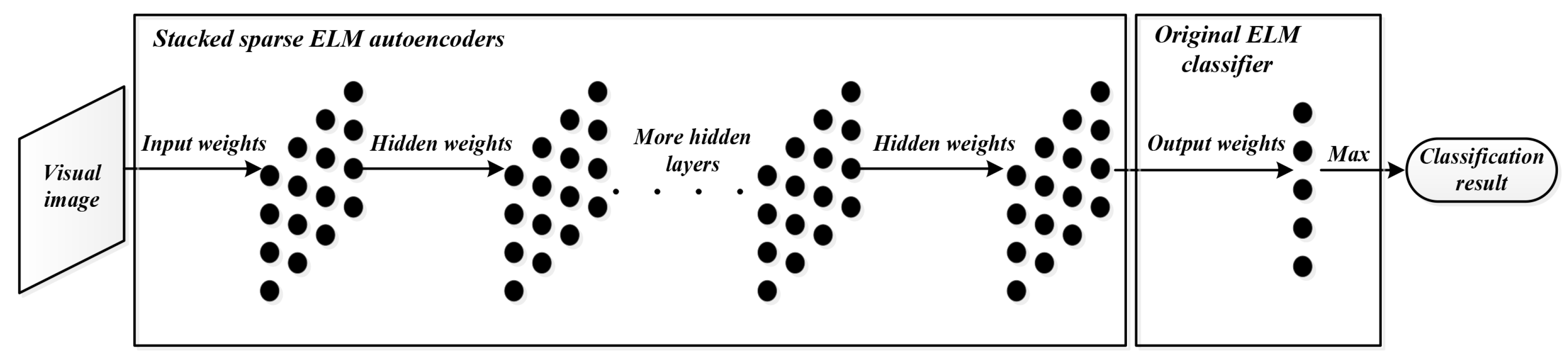replaced the $l_2$ norm constrain to the cost function of training the ELM-based autoencoder with $l_1$ optimization and made use of the FISTA algorithm [21] proposed by Beck and Teboulle to train a novel sparse ELM-based autoencoder. When stacked up and then combined with the conventional ELM classifier, such sparse ELM-based autoencoders form a multilayer network named hierarchical extreme learning machine (HELM [22]). It is reported that HELM has reached a higher recognition accuracy and is much faster than both conventional ELM-based methods and most deep learning methods on the mixed national institute of standards and technology database (MNIST [23]) and the NORB database [24].

However, the input weights and biases of the hidden nodes in ELM are generated according to a random distribution, which maps the inputs into the random feature space and may lead to the occurrence of non-optimal and redundant parameters that deteriorate discriminative features, which will have a bad influence on the final classification effect. In this paper, a hybrid method called the evolutionary hierarchical extreme learning network is proposed. Altogether, the main contribution is two-fold. Firstly, a novel sparse autoencoder is proposed by combining modified differential evolution with ELM so as to train a superior autoencoder with optimized hidden layer parameters and output weights, which makes the encoded features more discriminative. Secondly, the proposed evolutionary sparse ELM autoencoder is further integrated into a hierarchical network and realizes an end-to-end feature learning for object recognition with raw visible light camera sensor images. Experiments on two benchmarks (MNIST and NORB) show that the proposed method is able to obtain competitive or better performance than current relevant methods with acceptable or less time consumption.

The organization of the remaining sections are as follows. The preliminaries and research background are briefly introduced in Section 2. The details of the proposed method are described in Section 3. The experimental results and relevant analysis are given in Section 4, and Section 5 draws the final conclusion.

2. Background and Preliminaries

2.1. Differential Evolution

Differential evolution [25] (DE) was proposed by K. Price and R. Storn in 1997. It is an efficient heuristic member of the evolution algorithm family. DE shares the pipeline of common evolution algorithms (i.e., the composition of population initialization, fitness evaluation, individual mutation, crossover and selection), which is inspired by the natural biological evolution process, but it differs from other evolution algorithm members mainly in the way of mutating individuals. For any individual in the population of the k-th generation $x_i^k$, its corresponding mutated individual is given by Equation (1).

$$m_i^k=x_i^k+C_m(x_p^k-x_q^k)$$

(1)

where $C_m\in [0,2]$ is the mutation strength factor, the mutation comes from the weighted difference between two other randomly-chosen individuals $x_p^k$ and $x_q^k$, which makes DE a simple, but powerful self-organizing algorithm.

In more detail, Figure 1 illustrates the whole flowchart of DE, where there are six steps.

• Initialize the population randomly or according to some specific distribution.
• Pick out two individuals from the population randomly and compute the weighted difference.
• Carry out the mutation according to Equation (1).
• Conduct crossover between the mutated and the original individuals.
• Evaluate the fitness values of all the individuals in both the original population and the one after crossover.
• Select individuals according to the fitness values to form the population of the next generation.

2.2. Hierarchical Extreme Learning Machine

Generally, the proposal of ELM aims to train Single hidden layer feedforward networks (SLFNs). The universal approximation capability of ELM enables it to work well with a variety of features, and ELM or its variants usually work as a classifier in most applications. Tang et al. promoted ELM by proposing the hierarchical extreme learning machine (HELM), which integrates feature extraction and classification in one multilayer network. As Figure 2 shows, HELM is made up of two parts. One is the stacked sparse ELM autoencoders for unsupervised hierarchical feature learning, and the other is the conventional ELM classifier. Suppose that $\mathit{X}=\{{\mathit{x}}_i\in {\mathit{R}}^d,i=1,2,\dots ,N\}$ is the training dataset; the sparse ELM autoencoder in HELM tries to minimize the reconstruction error together with the norm of the output weights.

$${\mathit{F}}_{object}=\underset{\mathit{\beta }}{\arg \min }\{{\parallel \mathit{A}\mathit{\beta }-\mathit{X}\parallel }^2+{\parallel \mathit{\beta }\parallel }_{l_1}\}$$

(2)

where $\mathit{A}$ is the random hidden activation matrix given by Equation (3). The constraint on the norm of the output weights $\mathit{\beta }$ is $l_1$ instead of the commonly-used $l_2$ optimization. The reason for choosing the $l_1$ norm instead of the $l_2$ norm is that it is hoped to force the autoencoder to learn more sparse and compact features and reduce the needed number of hidden nodes.

$$\mathit{A}=\left[\begin{array}{ccc}\mathit{a}({\mathit{w}}_1·{\mathit{x}}_1+b_1)& \cdots & \mathit{a}({\mathit{w}}_M·{\mathit{x}}_1+b_M)\\ ⋮& \mathit{a}({\mathit{w}}_j·{\mathit{x}}_i+b_j)& ⋮\\ \mathit{a}({\mathit{w}}_1·{\mathit{x}}_N+b_1)& \cdots & \mathit{a}({\mathit{w}}_M·{\mathit{x}}_N+b_M)\end{array}\right]$$

(3)

where M is the hidden node number, ${\mathit{w}}_j$, $b_j$ are the corresponding input weight, bias and activation function of the j-th hidden node and $\mathit{a}(·)$ is the activation function.

$$\mathit{A}\mathit{\beta }=\mathit{X}$$

(4)

Since it is demonstrated in [26] that ELM has the universal approximation capability once the inputs are projected into random feature space, the encoding and decoding processing of the sparse ELM autoencoder in HELM can be treated as a linear system (see Equation (4)), and the expected output weights $\mathit{\beta }$ can be solved by following the ELM theory and applying the FISTA algorithm (more details could be found in [22]). Then, the encoded features are computed below.

$$\mathit{Y}=\mathit{a}(\mathit{X}·\mathit{\beta })$$

(5)

3. Evolutionary Hierarchical Extreme Learning Network

Feature representation is crucial to solving the objection recognition problem. It is able to extract discriminative information from raw data while removing the irrelevant or reductant data. The success of HELM lies in that the features encoded by the ELM autoencoder network are sparse and discriminative. Even though generated randomly, the hidden layer parameters in the ELM autoencoder network are related to the solution of the output weights (see Equation (1)), which are used for feature encoding. Zhu et al. [27] stated that random hidden layer parameters are not ideal and will result in the emergence of non-optimal unnecessary parameters. In [28], singular value decomposition is applied to optimize the randomly-set hidden layer parameters, and the final performance gets promoted significantly. Thus, for the purpose of achieving the improvement on the feature encoding and finally the recognition precision, the hidden layer parameters should be carefully selected and optimized.

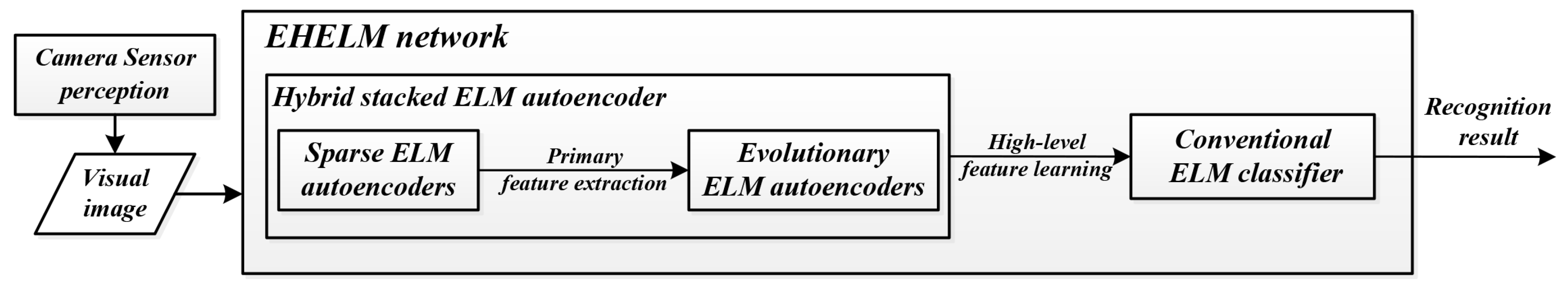
In this section, the proposed evolutionary hierarchical extreme learning network (EHELN) is presented. It can be seen in Figure 3 that there are two main modules composing the whole network, i.e., the classification module and the feature learning module. The former is actually a conventional ELM classifier. The latter is made up of two different autoencoders, i.e., the sparse ELM autoencoder in [22] for primary feature extraction, as well as dimensionality reduction, and the evolutionary sparse ELM autoencoder for high-level feature learning. During the training of the evolutionary sparse ELM autoencoder, the hidden layer parameters are searched by using differential evolution other than being randomly chosen in order to learn a more complete set of features with satisfactory discriminative capability. The next subsections will describe the details of the learning procedure of the evolutionary sparse ELM autoencoder.

3.1. Initialize the Population and Define the Fitness Function

Since the object to be optimized is the hidden layer parameters in the sparse ELM autoencoder, the definition of the individual in the initial population is direct and simple, i.e., the concatenation of the input weight and bias of each hidden node.

$$\mathit{\theta }=[{\mathit{w}}_1,{\mathit{w}}_2,{\mathit{w}}_j,\dots {\mathit{w}}_N,b_1,b_2,b_j\dots ,b_N]$$

(6)

where ${\mathit{w}}_j$ is the input weight and $b_j$ is the bias of the j-th hidden node, which are randomly initialized within [−1,1], and N is the hidden node number.

Following the ELM theory and HELM [22], each individual can be taken to compute analytically the sparse output weight with minimum norm by applying the FISTA algorithm [21]. There is no need to implement any backpropagation-based tuning, which is time-consuming and commonly utilized in deep learning.

The autoencoder aims to learn the feature space transformation that enables it to realize the reconstruction of the input data with minimized error. What is more, the learned features are expected to be discriminative enough, which means in the learned feature space, the data’s inter-distance should be as large as possible, while the intra-distance should be small. Therefore, the fitness function is defined to have two opponents, i.e., the reconstruction fitness ${\mathit{F}}_r$ and the discriminative fitness ${\mathit{F}}_d$, which are given in Equation (7).

$${\mathit{F}}_{\mathit{\beta },\mathit{\theta }}={\mathit{F}}_r\left(\mathit{\beta }\right)+{\mathit{F}}_d(\mathit{\theta },\mathit{\beta })$$

(7)

where $\mathit{\beta }$ refers to the output weight when taking $\mathit{\theta }$ as the hidden layer parameters. As shown by Equation (8), ${\mathit{F}}_d$ is actually the ratio of the inter-class distance $d_{inter}$ and the intra-class distance $d_{intra}$. Apparently, if the learned features are more discriminative, the values of ${\mathit{F}}_d$ will be higher so that data from different classes can be separated more easily.

$$p\left(\mathit{\beta }\right)=\frac{d_{intra}}{d_{inter}}=\frac{{\displaystyle \sum _{i=1}^{N_c}}{n}_i{∥{\mathit{m}}_i-\mathit{m}∥}^2}{{\displaystyle \sum _{i=1}^{N_c}}{\displaystyle \sum _{{\mathit{x}}_f\in c_i}}{∥{\mathit{x}}_f-{\mathit{m}}_i∥}^2}$$

(8)

where ${\mathit{X}}_f$ is the encoded feature belonging to the i-th class, which is calculated by Equation (5), $n_i$ is the number of samples in the i-th class, $N_c$ is the number of classes and ${\mathit{m}}_i$ stands for the mean value of the features in the i-th class.

$${\mathit{m}}_i=\frac{1}{n_i}\sum _{{\mathit{x}}_f\in c_i}{\mathit{x}}_f,\mathit{m}=\frac{1}{M}\sum _{i=1}^{Nc}{n}_i{\mathit{m}}_i$$

(9)

where $\mathit{m}$ is the mean value of the whole features and M is the total number.

Meanwhile, the reconstruction fitness ${\mathit{F}}_r$ is defined in Equation (10).

$$f(\mathit{\theta },\mathit{\beta })=1-\sqrt{\frac{{\displaystyle \sum _{j=1}^M}{∥\mathit{a}({\mathit{x}}_{\mathit{j}}\odot \mathit{\theta })\mathit{\beta }-{\mathit{x}}_{\mathit{j}}∥}_2^2}{D\times M}}=1-\sqrt{\frac{{\displaystyle \sum _{j=1}^M}{∥{\displaystyle \sum _{i=1}^N}\mathit{a}({\mathit{x}}_{\mathit{j}}·{\mathit{w}}_{\mathit{i}}+b_i)\mathit{\beta }-{\mathit{x}}_{\mathit{j}}∥}_2^2}{D\times M}}$$

(10)

where D is the dimension of ${\mathit{x}}_j$ and ⊙ denotes the linear mapping operation of each hidden node.

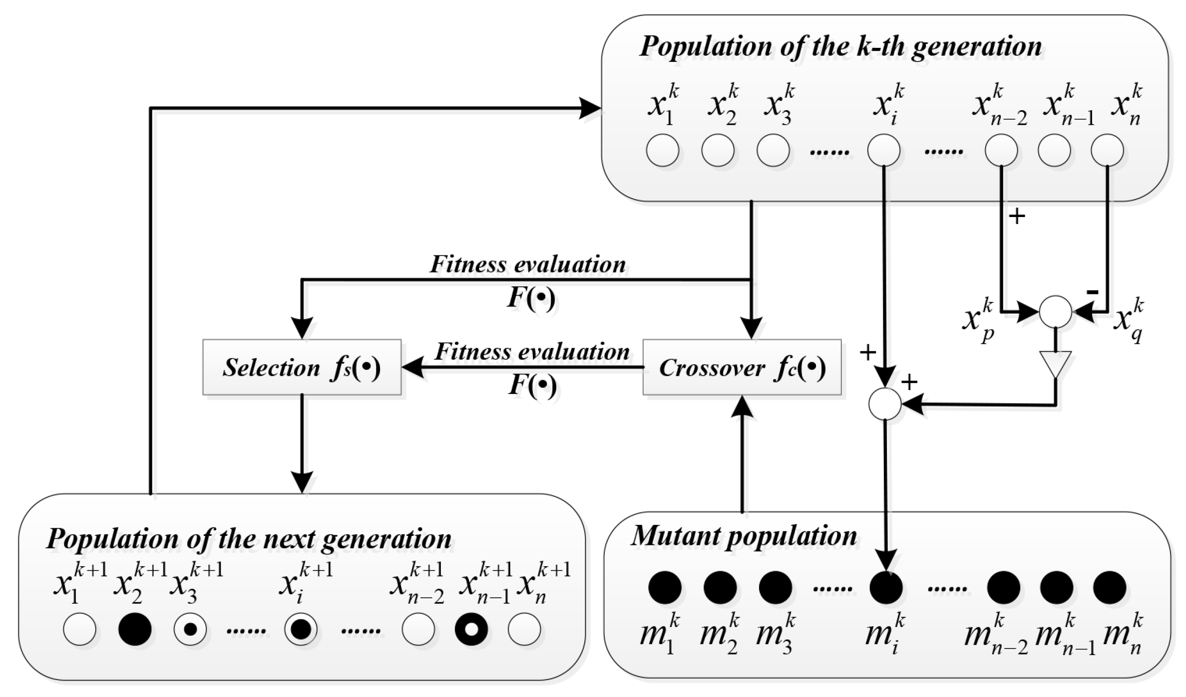
3.2. Mutate and Crossover the Individuals

According to differential evolution, the mutation is self-organizing, which means the variation comes from the difference between individuals themselves. For any individual, the corresponding mutated one is generated by Equation (10).

$${\mathit{m}}_{{\mathit{\theta }}_i}={\mathit{\theta }}_i+C_m(\Delta {\mathit{\theta }}_{r1}+\Delta {\mathit{\theta }}_{r2})$$

(11)

where ${\mathit{m}}_{{\mathit{\theta }}_i}$ is the mutated individual, ${\mathit{\theta }}_i$ is the original individual, $\Delta {\mathit{\theta }}_{r1}$ and $\Delta {\mathit{\theta }}_{r2}$ represent the difference of two pairs of other individuals, which are chosen randomly, and $C_m$ is a constant used to control and adapt the mutation strength.

$${\mathit{\mu }}_{{\mathit{\theta }}_i,k}=\left\{\begin{array}{cc}\hfill {\mathit{\theta }}_{i,k}& if{\mathit{f}}_{rand}<C_{co}\hfill \\ \hfill {\mathit{m}}_{{\mathit{\theta }}_i,k}& else\hfill \end{array}\right.$$

(12)

Then, as shown in Equation (12), the crossover is conducted among the attributes of the original individuals and the mutated ones, where ${\mathit{\theta }}_{i,k}$ and ${\mathit{m}}_{{\mathit{\theta }}_i,k}$ are the k-th attribute of the original individual and its mutated individual, respectively, ${\mathit{\mu }}_{{\mathit{\theta }}_i,k}$ is the crossover attribute, $C_{co}$ is the crossover factor and ${\mathit{f}}_{rand}$ is a function of a random number generator that gives the output within (0,1).

3.3. Select Predominant Individuals

At last, superior individuals from the augmented population, which contains both the original individuals and their corresponding mutated and crossover ones, will be picked out to form the population of the new generation. The superiority of the individuals is measured by the fitness function. The individual owning a larger fitness value has a higher probability to be selected. Moreover, Bartlett [29] has proven that the norm of weights in neural networks has a specifically important effect on the generalization performance, and the smaller the better. Taking this into consideration, when there exist individuals with similar fitness values, the one that leads to the output weight of the smaller norm will be chosen. Note that the fitness value of each individual is calculated on the basis of a subset of the whole training set to reduce computation consumption and avoid overfitting.

4. Experimental Results and Discussion

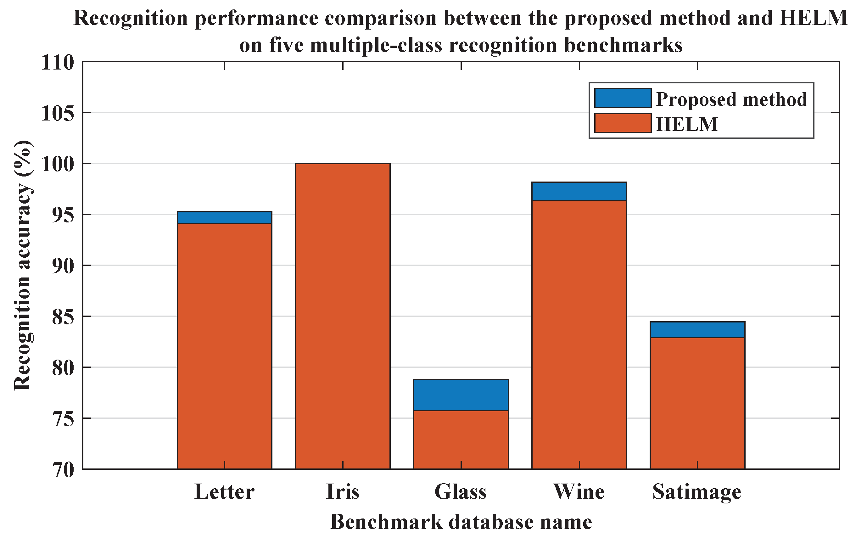
In this section, the proposed method is evaluated and compared with other related methods when applied to object recognition tasks on several typical benchmarks. The idea of the proposed evolutionary hierarchical sparse extreme learning autoencoder network was inspired by HELM, but it differs from HELM in that a hybrid stacked sparse autoencoder module, which is composed of evolutionary and conventional sparse ELM autoencoders, is integrated into the whole network for the extraction of more discriminative features oriented toward specific tasks. Firstly, the performance of the proposed method was evaluated and compared with HELM on five common multiple-class recognition databases preliminarily. The results are illustrated in Figure 4. The corresponding network configuration is given by

Table 1. Network configuration of the proposed method and HELM on different benchmark datasets.

Benchmark Database Name	Number of Hidden Nodes in Each Layer
Letter	L1 = L2 = 200, L3 = 2000
Iris	L1 = L2 = 20, L3 = 200
Glass	L1 = L2 = 20, L3 = 200
Wine	L1 = L2 = 20, L3 = 500
Satimage	L1 = L2 = 100, L3 = 1000

, where L1 and L2 are the hidden node numbers of each stacked ELM autoencoder and L3 of the conventional ELM classifier.

Clearly, except achieving the same 100% recognition accuracy on the Iris database, the performance of the proposed method was almost better than that of HELM. Note that when conducting the training of networks on each database, the network settings of both the proposed method and HELM were the same. Therefore, it could be concluded that the evolutional sparse ELM autoencoder whose hidden layer parameters get optimized by differential evolution outperformed the conventional ones used by HELM, and compared with HELM, the proposed evolutionary hierarchical sparse extreme learning autoencoder network was able to extract features equipped with better discriminative capability, which finally helped to improve the recognition accuracy.

Next, two representative object recognition benchmarks were used for further performance comparisons. Comparative methods include the ELM-based ML-ELM [19], HELM [22], as well as the DL-based SAE [4], SDA [30], DBN [31] and DBM [32]. The learning rate of the DL-based methods was 0.1, and the decay rate was 0.95. As for SDA, the corruption rate was set as 0.5, while the drop rate was 0.2. In ML-ELM, there were three hidden layers in all, the $l_2$ penalty coefficients of which were ${10}^{-1}$, ${10}^3$ and ${10}^8$, respectively. The mutation strength constant and the crossover factor used in the proposed method were 1 and 0.8 correspondingly. Except that the pixel values of the input raw images were normalized to [−1,1], no other image preprocessing was conducted.

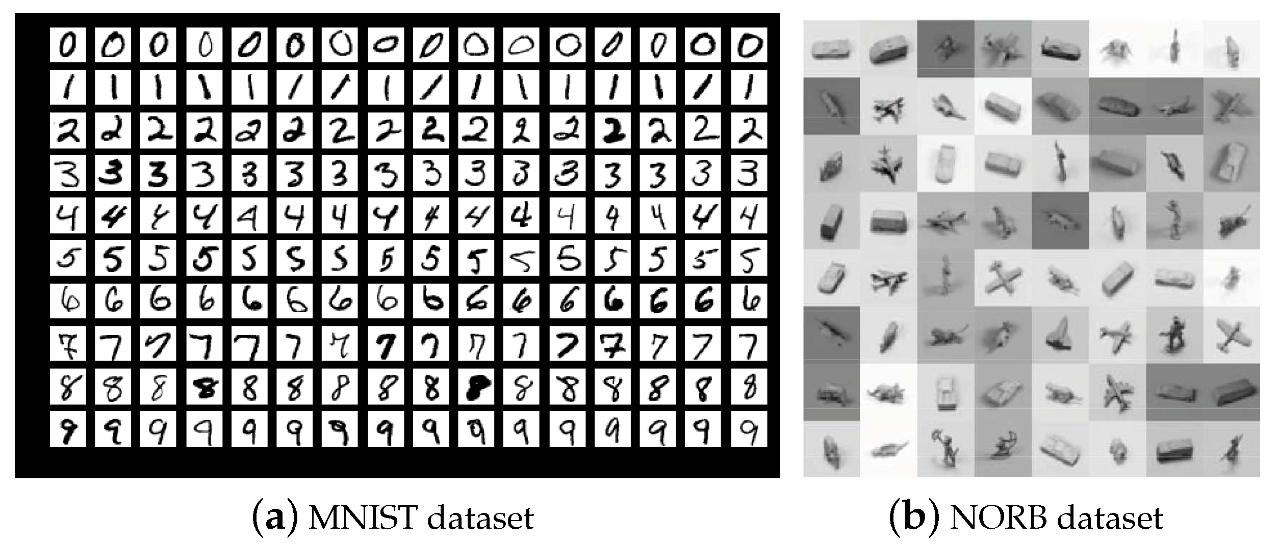
The MNIST 2D handwritten digit recognition database and NORB 3D object recognition database were used in comparative experiments, both of which are the representative benchmarks for evaluating object recognition algorithms. The MNIST consists of 70,000 grayscale $28\times 28$ images of handwritten digits collected from 500 people (see Figure 5a). There are 60,000 images in the training set, each of which contains a digit from 0–9. The MNIST requires nearly no formatting and preprocessing and is a practical platform for real-world objection recognition application. Meanwhile, the NORB dataset is more challenging than the MNIST and oriented toward recognizing 3D objects under different imaging conditions (see Figure 5b). It comprises 97,200 images of 50 3D toys that belong to five major categories, such as animals, planes, and so on. All the images were captured by two visible light cameras set at 9 azimuths and 36 angles under 6 different lighting conditions.

4.1. Comparison with HELM and Analysis

At first, the proposed method was compared with the HELM so as to validate that the evolutionary sparse ELM autoencoder used in the proposed method did help improve the performance. With regards to this, except for changing the hidden node number of the evolutionary sparse ELM autoencoder, the other network architectures of the proposed evolutionary hierarchical extreme learning network were the same as those of the HELM. For the MNIST dataset, the number of hidden nodes of the sparse ELM autoencoder and ELM classifier was 700 and 12,000, respectively, while 3000 and 15,000 for the NORB dataset. The regularization parameter C was $2\times {10}^{-30}$.

Table 2. Recognition accuracy (%) vs. different hidden nodes of the proposed method and HELM on the MNIST dataset.

Hidden Node Number	300	400	500	600	700	800	900
HELM	0.9895	0.9893	0.9890	0.9899	0.9913	0.9892	0.9891
the proposed method	0.9917	0.9920	0.9919	0.9119	0.9923	0.9919	0.9919

and

Table 3. Recognition accuracy (%) vs. different hidden nodes of the proposed method and HELM on the NORB dataset.

Hidden Node Number	1000	1500	2000	2500	3000	3500	4000
HELM	0.9021	0.8984	0.9026	0.9001	0.9128	0.9004	0.9007
the proposed method	0.9123	0.9120	0.9119	0.9136	0.9246	0.9118	0.9117

show the recognition accuracy varying with the number of hidden nodes in the conventional sparse ELM autoencoder in HELM and the evolutionary sparse ELM autoencoder in the proposed method on the MNIST dataset and the NORB dataset, respectively.

Apparently, it can be illustrated that with the same number of hidden nodes the recognition precision of the proposed method was always higher than HELM. Increasing the hidden node number helps to improve the performance, but overfitting will happen if the hidden node number is too large. The proposed method could reach the same recognition accuracy as that of HELM, but called for less hidden nodes. This should benefit from the optimized hidden layer parameters obtained by differential evolution during the learning procedure of the the evolutionary sparse ELM autoencoder.

Furthermore, the highest level features encoded by the last sparse ELM autoencoder in HELM and the evolutionary sparse ELM autoencoder in the proposed method were taken out, and the discriminative rate given in Equation (8) was adopted to measure how discriminative the features were quantitatively, which is given in

Table 4. Discriminative rate comparison of the features encoded by the proposed method and HELM on the MNIST dataset.

Method	HELM	The Proposed Method
Discriminative rate	0.9274	0.9372

and

Table 5. Discriminative rate comparison of the features encoded by the proposed method and HELM on the NORB dataset.

Method	HELM	The Proposed Method
Discriminative rate	0.4711	0.4724

. Clearly, the discriminative rates of the features encoded by the proposed method (0.9372 on MNIST and 0.4724 on NORB) were higher than those encoded by HELM (0.9274 on MNIST and 0.4711 on NORB). It can be concluded that the hidden layer parameters did impact the feature encoding of the ELM-based autoencoder, and the encoded features of the proposed method were more discriminative and can provide more useful information for building classifiers with good generalization capability. This could be the clue to explain the results shown in Table 2 and Table 3.

4.2. Comparison with Relevant State-of-the-Art Methods and Analysis

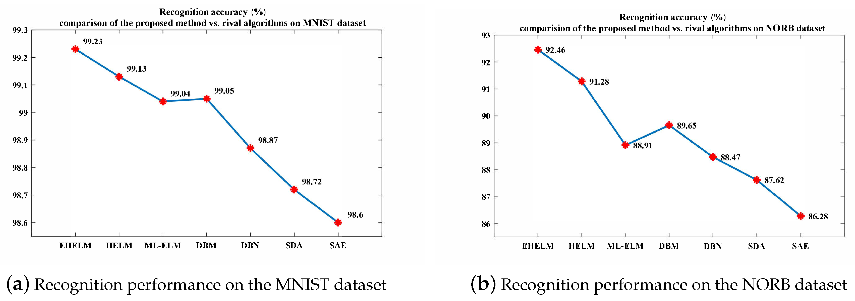
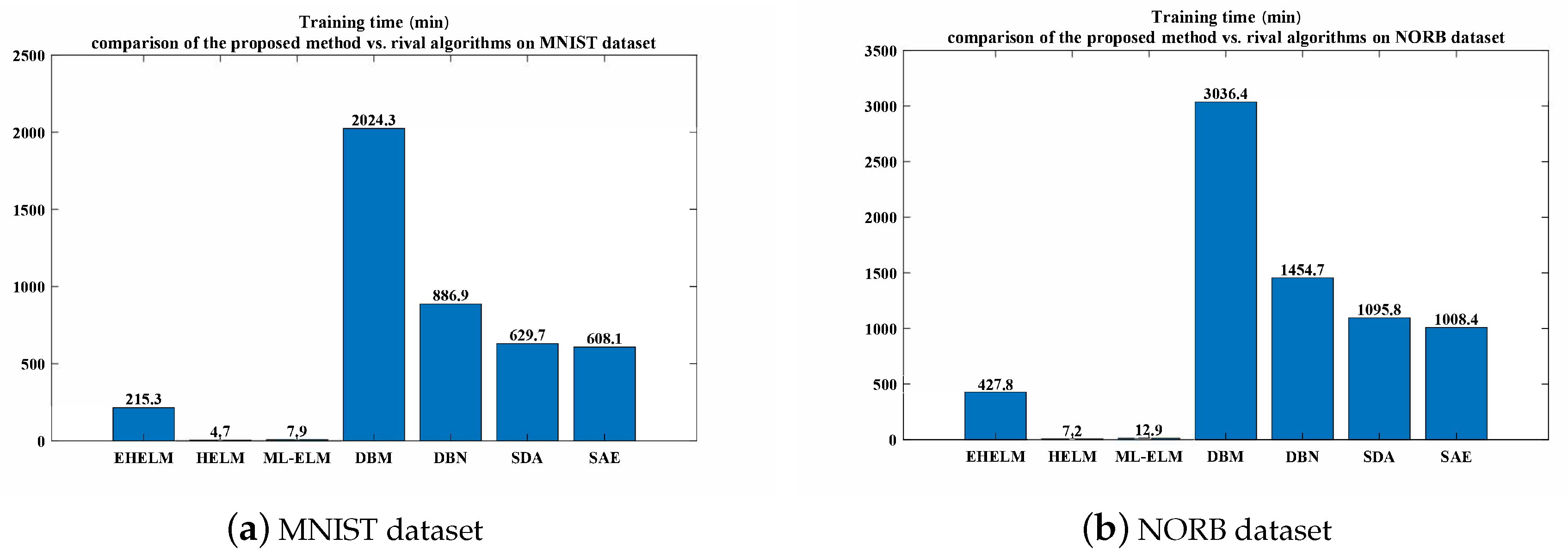
Next, both the performance and the training cost of the proposed method were compared with those of relevant state-of-the-art methods, which are given by Figure 6 and Figure 7. In terms of recognition accuracy, the proposed method obtained the best results (i.e., 99.23% on MNIST and 92.46% on NORB), followed by HELM, DBM and then the ML-ELM and the like. Since it can be inferred from the aforementioned experimental comparison and analysis that the improved performance of the proposed method was derived from differential evolution, more computation was needed for searching the optimized hidden layer parameters such that it required a longer training phase than what other ELM-based methods do. However, differential evolution was only applied to the evolutionary sparse ELM autoencoder, which was stacked at higher layers of the whole network for high-level feature extraction. The learning of other modules in the proposed method still followed the ELM theory. Hence, the computation cost became larger, but acceptable. Compared with ELM-based methods, the training period of the proposed method was much longer, but was about at least two- or three-times faster than the DL-based methods.

4.3. Application on a Real Complex Dataset

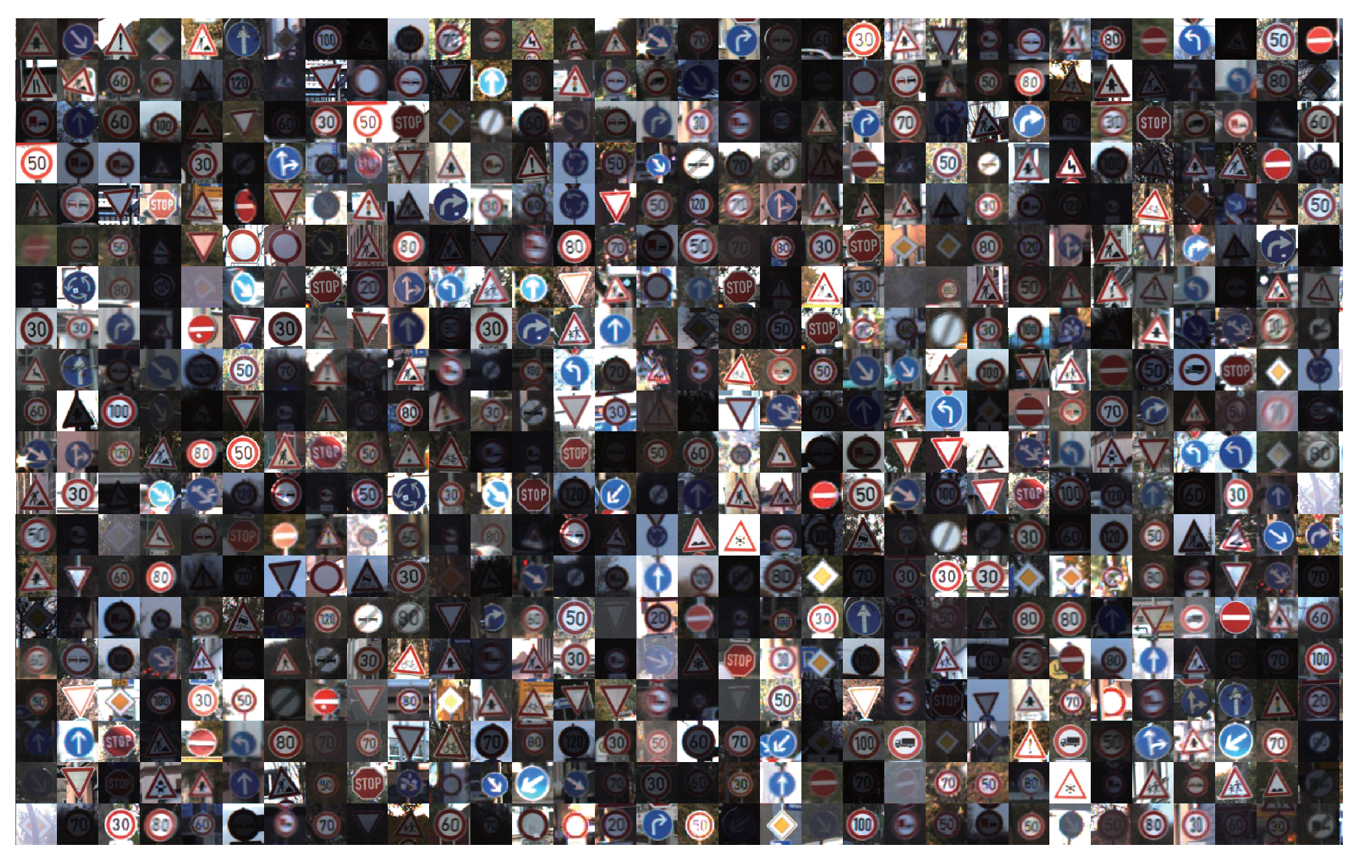
For the purpose of demonstrating the applicability of the proposed method on a real complex recognition task, the German traffic sign recognition benchmark (GTSRB [33]) was chosen as the test dataset, which contains more than 50,000 images of traffic signs captured in various real scenes and weather situations. The images in GTSRB suffer from issues such as contrast degradation, occlusion, over exposure, distortion, and so on. All the traffic signs belong to 43 classes in all (see Figure 8), the size of which ranges from $15\times 15$ to $250\times 250$.

The network structure of the proposed method here is in accordance with the one used in the experiments on MNIST and NORB datasets, that is two sparse ELM autoencoders for feature encoding and one ELM classifier for feature classification. Before applying the proposed method, all the traffic sign images were resized to $48\times 48$ and centered to have mean value of zero and scaled to have a standard deviation of one. The ZCA whiten procedure was conducted to normalize all the image samples, which were then fed to the proposed method for training and testing. The final results of recognition rates were recorded. The relevant rival methods that had formal reported results on GTSRB were also given, including HOG-LDA [33], HOG-random forests [34], BW-ELM [35], HELM [22] and HOGv-ELM [15]. As is shown in

Table 6. Recognition performance comparison with relevant rival methods on the GTSRB dataset.

Method	HOG-LDA	HOG-Random Forests	BW-ELM	HELM
Accuracy (%)	95.68	96.14	97.19	97.85
Method	Human Performance	HOGv-ELM	Proposed Method
Accuracy (%)	98.84	99.09	98.91

, the proposed method owned the second highest recognition accuracy of 98.91%, that is 0.18% lower than the best result of HOGv-ELM. Note that HOGv-ELM is based on the variant version of HOG features that is specifically designed for representing traffic signs, while the proposed method learned the feature representation directly from raw inputs. The proposed method outperformed other methods with a recognition rate that was better than human performance. Such a result could to some extent demonstrate that the proposed method was meaningful and useful for real practical application.

5. Conclusions

In this paper, a novel evolutionary sparse ELM autoencoder was proposed and embedded in the hierarchical neural network called the evolutionary hierarchical sparse extreme learning autoencoder network. Due to the training of the whole network being based on least mean squares, it is faster and requires less computation than rival deep learning methods while maintaining great performance. Besides, since the parameters in the hidden layer of the sparse ELM autoencoder are optimized by differential evolution other than being generated randomly, the discriminative ability of the encoded features get further strengthened, so that the proposed method can outperform previous ELM-based opponents with acceptable time consumption when applied to object recognition problems. Experimental results on typical benchmarks have also validated the proposed method’s utility and capability.

Since it is reported that ELM with a local receptive field and combinational node has achieved impressive results superior to state-of-the-art methods including convolutional neural networks, the future work should extend the proposed evolutionary sparse ELM autoencoder to such a new ELM structure so as to further improve the quality of the feature encoding. In the meantime, more challenging tasks and data such as the ones perceived by the visible light camera mounted on real cars will also be used to test the proposed method’s robustness and generalization performance.