Vertex Labeling and Routing for Farey-Type Symmetrically-Structured Graphs

Abstract

The generalization of Farey graphs and extended Farey graphs all originate from Farey graphs. They are simultaneously scale-free and small-world. A labeling of the vertices for them are proposed here. All of the shortest paths between any two vertices in these two graphs can be determined only on their labels. The number of shortest paths between any two vertices is the product of two Fibonacci numbers; it is increasing almost linearly with the order or size of the graphs. However, the label-based routing algorithm runs in logarithmic time O(logn). Our efficient routing protocol for Farey-type models should help contribute toward the understanding of several physical dynamic processes.

1. Introduction

In comparison with empirical and random graphs, deterministic models have unique advantages in improving our comprehension in complex networks. For instance, we can obtain the solutions for a deterministic model by rigorous derivation, and the computation is only a small quantity of calculations. Deterministic models can be created by simple recursive operation [1,2,3,4], construction of fractal processes [5], plane filling techniques [6], the relationships between natural numbers [7], or perspectives and methods from classical research of physical processes [8,9,10,11]. Recently, Zhang et al. introduced Farey graphs (FG) on the basis of classical Farey sequences. Farey graphs are simultaneously uniquely Hamiltonian, minimally three-colorable, maximally outer-planar, and perfect [12,13]. FG can be used as modules of multiple networks. The networks created by edge iterations [14], or evolving graphs with geographical attachment preference [15], coincide with the combination of three FG, while the merger of six FG generates graphs with multidimensional growth [16]. Moreover, two new kinds of Farey-type graphs, the generalization of Farey graphs (GFG), and the extended Farey graphs (EFG) are deduced by generalizing the construction mechanism of FG, and they all are scale-free and small-world [17,18,19].

Deterministic graphs also provide a new perspective and methodology for classical research of physical processes. For example, some important dynamical processes on the basis of Apollonian models [20], a kind of deterministic matching graph, space-filling, Euclidean, small-world, and scale-free, has been researched extensively. Accurate analytical solutions are derived, including percolation [21], electrical conduction [20], Ising models [20], quantum transport [22], partially connected feedforward neural networks [23], traffic gridlock [24], Bose–Einstein condensation [25], free-electron gas [26], and so on. However, the study of physical processes using FG is still lacking, as the recursive relationships in FG are more complex than for Apollonian networks.

The label-based routing protocol for all shortest paths may also bridge Farey-type graphs with the fields below. The all-pairs shortest paths problem is frequently studied in textbooks and it has remained open to this day, the classical algorithms such as the A*, Bellman–Ford, Floyd–Warshall and Dijkstra algorithms all run in subcubic time $O({\left|V\right|}^{3-\delta })$, where $\delta >0$ [27,28,29,30,31]. The $K$ shortest path routing (KSPR) algorithm is an extension of the shortest path routing algorithm, in which $K$ is the number of shortest paths to find [32]. KSPR finds K paths in order of increasing cost, including the shortest path. KSPR in Farey-type graphs will partly reduce to finding out all the shortest paths. Similar to the minimum spanning problem, the graph Steiner tree problem (GSTR) interconnects a set $V$ of vertices by using a network of shortest length, and the length is the sum of the lengths of all edges [33]. Most versions of GSTR are NP (non-deterministic polynomial) complete. Moreover, the bottleneck of many network analysis algorithms is the exorbitant computational complexity of calculating the shortest paths, so that scientists are forced to use approximation algorithms [34].

Graph labeling is one active subject in graph theory. Graph labeling has a wide range of applications in many fields, such as communication design, circuit design, crystallography, and coding theory [35]. Finding the shortest paths in graphs is an open problem, which has been well studied. Zhang and Camellas pioneered the relationship between the shortest paths and vertex labels [35,36,37,38,39]. They can determine the shortest path just by applying simple rules and a few computations based only on their labels.

We propose an algorithm for labeling nodes—all of the shortest paths between any pair of vertices can be efficiently derived only on the basis of their labels. We found that the number of shortest paths between two vertices is huge, but the routing algorithm runs in logarithmic time O(logn).

Furthermore, the existence of symmetry in real-world graphs have been underlined by analyzing of over 1500 graph datasets [40,41,42,43]. It was found that over 70% of the empirical networks contain symmetries, independent of size and modularity. All the graphs we proposed here are symmetrically-structured on the basis of Farey-type graphs, and therefore our labeling and routing algorithms can provide a new viewpoint on empirical networks which are containing symmetries.

2. Generation of Farey-Type Graphs

GFG and EFG are generalized from FG; we present the definitions of the three in turn.

Definition 1.

(Generation of FG) Farey graph $F(t)=(V(t),E(t))$ is constructed as follows (see Figure 1), in which the iteration step $t\ge 0$, with vertex set$V(t)$and edge set$E(t)$[6]:

• $F(0)$has two vertices and an edge.
• For$t\ge 1$,$F(t)$is obtained from$F(t-1)$by adding a new vertex to every edge which is introduced at step$t-1$in$F(t-1)$, then to linking the new vertex to the two vertices of that edge.

Remark 1.

The number of vertices added at step$t$is$\Delta n_t=2^{t-1}$, so that the order of FG is$\left|V(t)\right|=2^t+1$and the size is$\left|E(t)\right|=2^{t+1}+1$, respectively. The cumulative degree distribution follows an exponential distribution$P_{cum}(\delta )=2^{-\frac{\delta }{2}}$, and the degree correlation$k_{nn}(\delta )$is approximately a linear function of $\delta$ [6,7].

All the vertices in$F(t)$are divided into three groups by their distances to two initial vertices$X$and$Y$:$V^x(t)$,$V^{xy}(t)$and$V^y(t)$. The nodes in$V^y(t)$(including$Y$) have shorter distances to$Y$than to $X$, while$V^x(t)$(including$X$) have shorter distances to$X$, and in$V^{xy}(t)$the distances are equal. That is to say,$V(t)=V^x(t)\cup V^{xy}(t)\cup V^y(t)$. As$X$and$Y$are neighbors, the difference in distances above are 0 or 1. If two copies of$F(t)$are named as$F_1(t)$and$F_2(t)$, the initial vertices are$X_1$,$Y_1$and$X_2$,$Y_2$, then$F(t+1)$is generated as shown in Figure 2.

Definition 2.

(Generation of GFG)$GF(t,k)$is deduced by the rules (see Figure 3):

• For$t=0$,$GF(0,k)$is composed of three initial vertices which are linked to each other.
• For$t\ge 1$,$GF(t,k)$is constructed from$GF(t-1,k)$by adding$k$new vertices to every edge introduced at step$t-1$, then linking the$k$new vertices to the two end vertices.

Remark 2.

$GF(t,1)$is exactly the graphs created by edge iterations [8]. It is just the evolving graphs with geographical attachment preference [9]. GFG can also be treated as a flower, which has$3\times k$identical petals, denoting as$P_i(t)$,$i=1,2,\dots ,3\times k$. All petals are rooted from two initial vertices, as a GFG is made up of three groups, so that each group contains$k$identical petals.

Definition 3.

(Generation of EFG) The construction of$EF(t,k)$is shown as below:

• For$t=0$, $EF(0,k)$ holds three vertices that are linked to each other.
• For$t\ge 1$,$EF(t,k)$is constructed from$EF(t-1,k)$by adding$k$new vertices to every edge linked at step$t-1$and three initial edges added at$t=0$, then linking the$k$new vertices to the two end vertices (see Figure 4).

Remark 3.

The generation method of EFG is slightly different from GFG, which lies in the three initial edges, not only the edges merged at step $t-1$, but as active edges that can generate new vertices. EFG has$3\times t\times k$petals, named$P_i(t_j)$,$i=1,2,\dots ,3\times k$and$t_j=0,1,\dots ,t$; a GFG is therefore just part of an equivalent EFG.

3. Labeling and Routing of $F(t)$

The labeling and routing protocol of GFG and EFG are extended from FG; the label-based routing algorithm was originally derived in [33], but we redefine it here for completeness and clarity. In order to save space, we do not repeat the proofs of these properties in this section.

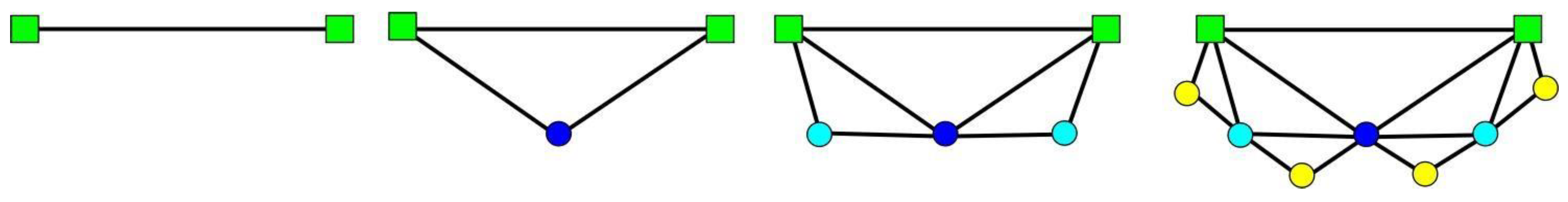
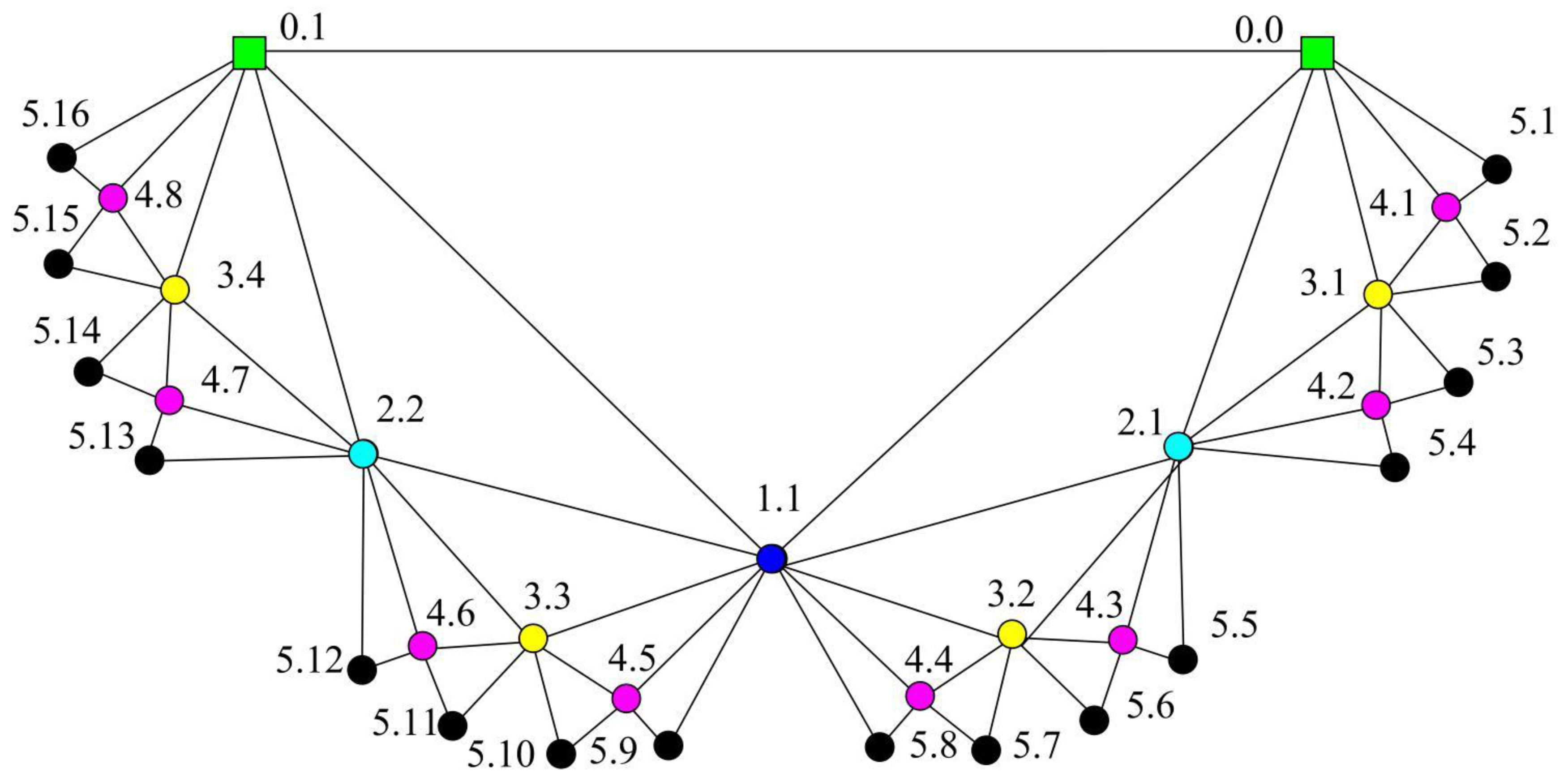
Definition 4.

Labeling any vertex in FG as follow (see Figure 5):

• Label two initial vertices as$0.1$and$0.0$when t = 0.
• When$t\ge 1$, the new vertices added at step t are marked with labels from$t.1$to$t{.2}^{t-1}$in a clockwise direction.

Supposing any two vertices are labeled with $t_i.k$ and $t_j.l$, and $t_i\ge t_j$. Then the mother vertex of $t_i.k$ added to the graph at step $t_i-1$. Two vertices with same mother are brothers. The father is added to the graph at step $t_i-2$ or earlier. The following relationships between different vertices, are extracted with the help of their labels.

Property 1.

(The family of $t_i.k$)

Two children of$t_i.k$are$(t_i+1).(2k-1)$and$(t_i+1).2k$when$t_i\ge 1$.

When$t_i\ge 2$,The brother of$t_i.k$is$t_i.(k+1)$(when$k$is odd) or$t_i.(k-1)$(when$k$is even).

When$t_i\ge 2$,$t_i.k$and its parents shapes a triangle. The mother is$(t_i-1).\lfloor \frac{k}{2}\rfloor$and the father is$(t_i-l).\lfloor \frac{k-rem(k,2)}{2^l}\rfloor$(in which$rem(k,2)$is the remainder of$k$divided by 2,$\lfloor x\rfloor =floor(x)$is a function rounding the real number$x$down towards the nearest integer. The integer$l(\ge 2)$is the number of the continuous zeros from right to left in the binary sequence created by converting the value of$k-rem(k,2)$to base 2, plus one, that is, l = Function(k-rem (k,2)).

If$t_i\ge t_j$, the$(t_i-t_j)th$generation of maternal ancestor of$t_i.k$is$t_j.\lfloor \frac{k}{2^{t_i-t_j}}\rfloor$.

Property 2.

(The neighbors of$t_i.k$)

When$t_i=0$, the neighbors of$0.0$is$\left\{x.1\right\}$,$x\in \{0,1,2,\dots ,t\}$, and the neighbors of$0.1$are$\{0.0,x{.2}^{x-1}\}$,$x\in \{1,2,\dots ,t\}$.

When$t_i=1$, the neighbors of$1.1$are$\{0.0,0.1,(1+x){.2}^{x-1}(2k-1),(1+x).[2^{x-1}(2k-1)+1]\}$,$x\in \{0,1,2,\dots ,t\}$.

When$t_i\ge 2$, the neighbors of$t_i.k$are$\{(t_i-l).$$\lfloor \frac{k-rem(k,2)}{2^l}\rfloor ,(t_i-1).\lfloor \frac{k}{2}\rfloor ,(t_i+x){.2}^{x-1}(2k-1),$$(t_i+x).[2^{x-1}(2k-1)+1]\}$,$x\in \{1,2,\dots ,$$t-t_i\}$.

Property 3.

When two vertices are located in different subgraphs$F_1(t-1)$and$F_2(t-1)$of$F(t)$, the hub$X$of$F(t)$is on the shortest paths, if

(1)$t_i.k\in V_2^x(t-1)$and$t_j.l\in V_1^y(t-1)/\left\{Y_1\right\}$,

(2) or$t_i.k\in V_1^x(t-1)$and$t_j.l\in V_2^y(t-1)/\left\{Y_2\right\}$,

(3) or$t_i.k\in V_2^x(t-1)\cup V_2^{xy}(t-1)$and$t_j.l\in V_1^x(t-1)\cup V_1^{xy}(t-1)$,

(4)$t_i.k\in V_1^x(t-1)\cup V_1^{xy}(t-1)$and$t_j.l\in V_2^x(t-1)\cup V_2^{xy}(t-1)$. Two initial vertices$Y_1$and$Y_2$of$F(t)$are located on the shortest paths if

(1)$t_i.k\in V_2^y(t-1)$and$t_j.l\in V_1^y(t-1)$,

(2) or$t_i.k\in V_1^y(t-1)$and$t_j.l\in V_2^y(t-1)$.

Vertices$X$,$Y_1$and$Y_2$lie on the shortest paths simultaneously if

(1)$t_i.k\in V_2^y(t-1)$and$t_j.l\in V_1^{xy}(t-1)$,

(a) or$t_i.k\in V_1^y(t-1)$and$t_j.l\in V_2^{xy}(t-1)$.

Property 4.

All the shortest paths between any pair of vertices are located a minimum common subgraph (MCSG) denoted as $F_{}^{mcsg}(t_{\min })$. Moreover, one vertex is an initial vertex or a$(p+1)th$layer vertex in$F_{3-\eta }^{mcsg}(t_{\min }-1)$, the other is positioned in the outermost layer of$F_{\eta }^{mcsg}(t_{\min }-1)$.

Property 5.

(The shortest paths routing algorithm of Farey graphs)

1. 

Given a pair of vertices labeled with$t_i.k$and$t_j.l$.

2. 

Determine whether the two vertices are neighbors or not.

If$t_i-t_j=1$and$l=\lfloor \frac{k}{2}\rfloor$, or$t_i-t_j=m$and$l=\lfloor \frac{k-rem(k,2)}{2^m}\rfloor$, by Property 1, the two vertices are in a mother-child or father-child relationship. Insert the two labels to the labels set of the shortest paths ($LSS{P}_m(h)$). Noticing that$LSS{P}_m(0)=\varnothing$and$m$is an integer increasing from one, go to step 6.

3. Find out MCSG when $l=\lfloor \frac{k}{2^{t_i-t_j}}\rfloor$, namely, where $t_j.l$ is the $(t_i-t_j)th$ generation of maternal ancestor of $t_i.k$.

If$k\in \{(l-1)\times 2^{t_i-t_j}+2^{t_i-t_j-1}+2\}$, or$k\in \{(l-1)\times 2^{t_i-t_j}+2^{t_i-t_j-1}+3,$$(l-1)\times 2^{t_i-t_j}+2^{t_i-t_j-1}+4\}$, or ..., or$k\in \{(l-1)\times 2^{t_i-t_j}+2^{t_i-t_j-1}+2^{t_i-t_j-2}+1,l\times 2^{t_i-t_j}\}$, MCSG is the embedded subgraph from$F(2)$to$F(t_i-t_j)$.$t_j.l$is the initial vertex$0.0$and$t_i.k$is an outermost layer vertex in MCSG.

If$k\in \{(l-1)\times 2^{t_i-t_j}+2^{t_i-t_j-1}-2\}$, or$k\in \{(l-1)\times 2^{t_i-t_j}+2^{t_i-t_j-1}-3,(l-1)\times 2^{t_i-t_j}+2^{t_i-t_j-1}-4\}$, or ..., or$k\in \{(l-1)\times 2^{t_i-t_j}+1,(l-1)\times 2^{t_i-t_j}+2^{t_i-t_j-1}\}$, MCSG is also the embedded subgraph from$F(2)$to$F(t_i-t_j)$, but$t_j.l$is the other initial vertex$0.1$. Go to step 5.

4. Find out MCSG when $l\ne m=\lfloor \frac{k}{2^{t_i-t_j}}\rfloor$.

If$t_j.m$is the$(t_i-t_j)th$generation of maternal ancestor of$t_i.k$, then$F_{}^{mcsg}(t_{\min })=F(t_i-t_j+p+1)$, in which$2^{p-1}\le \left|m-l\right|\le 2^p$. Go to step 5.

5. Determine whether $X$, $Y_1$ and $Y_2$ of MCSG are on the shortest paths or not.

Map the labels of$F_{}^{mcsg}(t_{\min })$onto labels of$F(t_{\min })$and divide all the vertices in$F(t_{\min })$into six sets as above:$V_{\eta }^x(t_{\min }-1)$,$V_{\eta }^{xy}(t_{\min }-1)$and$V_{\eta }^y(t_{\min }-1)$. Then, decide whether$X$,$Y_1$and$Y_2$are on the shortest paths by Property 3 or not.

If only the node$X$is on the paths, then insert the label of$X$, assuming the label is$t_p.q$, in the middle of$t_j.l$and$t_i.k$in$LSS{P}_m(h)$, and$h=h+1$. Thereafter, go back to step 1 with two new pairs of labels:$t_i.k$and$t_p.q$,$t_p.q$and$t_j.l$.

If only$Y_1$and$Y_2$are on the paths, insert the labels of$Y_1$and$Y_2$, being$t_{p1}.q1$and$t_{p2}.q2$respectively, in the middle of$t_i.k$and$t_j.l$in$LSS{P}_m(h)$, and$h=h+2$. Get two new pairs of labels,$t_i.k$and$t_{p1}.q1$,$t_{p2}.q2$and$t_j.l$, and go back to step 1.

If$X$,$Y_1$and$Y_2$are all on the paths at the same time, insert$t_p.q$into$LSS{P}_m(h)$and$h=h+1$, then insert$t_{p1}.q1$and$t_{p2}.q2$into$LSS{P}_{m+1}(h)$,$h=h+2$. Go back to step 1 with four pairs of labels:$t_i.k$and$t_p.q$,$t_p.q$and$t_j.l$,$t_i.k$and$t_{p1}.q1$,$t_{p2}.q2$and$t_j.l$.

6. Ascertain the shortest paths routing.

The shortest paths are traversed over every element in every set of$LSS{P}_m(h)$in order, where$m$is the number of the shortest paths and$h$is the distance between$t_i.k$and$t_j.l$.

Property 6.

The shortest paths routing algorithm in Property 5 between any two vertices of a Farey graph runs in logarithmic time.

Proof. 

Each algorithm has its time complexity and space complexity.

The space complexity of the shortest paths routing algorithm in Property 5 is decided by the number of shortest paths. The number is exactly the product of two Fibonacci numbers. When $t_i=t_j=t$, the max number is $F_{\lfloor \frac{t}{2}\rfloor +1}\times F_{\lfloor \frac{t-3}{2}\rfloor +1}=\frac{1}{5}[{(\frac{1+\sqrt{5}}{2})}^{\lfloor \frac{t}{2}\rfloor +1}-{(\frac{1-\sqrt{5}}{2})}^{\lfloor \frac{t}{2}\rfloor +1}][{(\frac{1+\sqrt{5}}{2})}^{\lfloor \frac{t-3}{2}\rfloor +1}-{(\frac{1-\sqrt{5}}{2})}^{\lfloor \frac{t-3}{2}\rfloor +1}]$, increasing almost exponentially [33]. The order and size of FG is $\left|V(t)\right|=2^t+1$, so the space complexity increases almost linearly with O(n).

However, the time complexity is determined by the maximum number of the vertices, which are located in the shortest paths in two Farey-type graphs. We can obtain that all the vertices on the shortest paths shape rhombuses which are zigzagged adjacent from the construction mechanism. The max number of rhombuses from $t_i.k$ to $0.\lfloor \frac{k}{2^{t_i-2}}\rfloor$ is $\lfloor \frac{t_i}{2}\rfloor$. While from $t_j.l$ to $0.\lfloor \frac{l}{2^{t_j-2}}\rfloor$ is $\lfloor \frac{t_j-3}{2}\rfloor$. That is to say, only at most $2t+1$ vertices need to be ascertained in the routing algorithm. When determining a vertex of $2t+1$ vertices, several operations of addition and multiplication are needed. For the order of FG is $\left|V(t)\right|=2^t+1$ and $\log \left|V(t)\right|\propto t$, all the shortest paths can be determined in logarithmic time $O(\log n)$. ☐

4. Labeling of $GF(t,k)$ and $EF(t,k)$

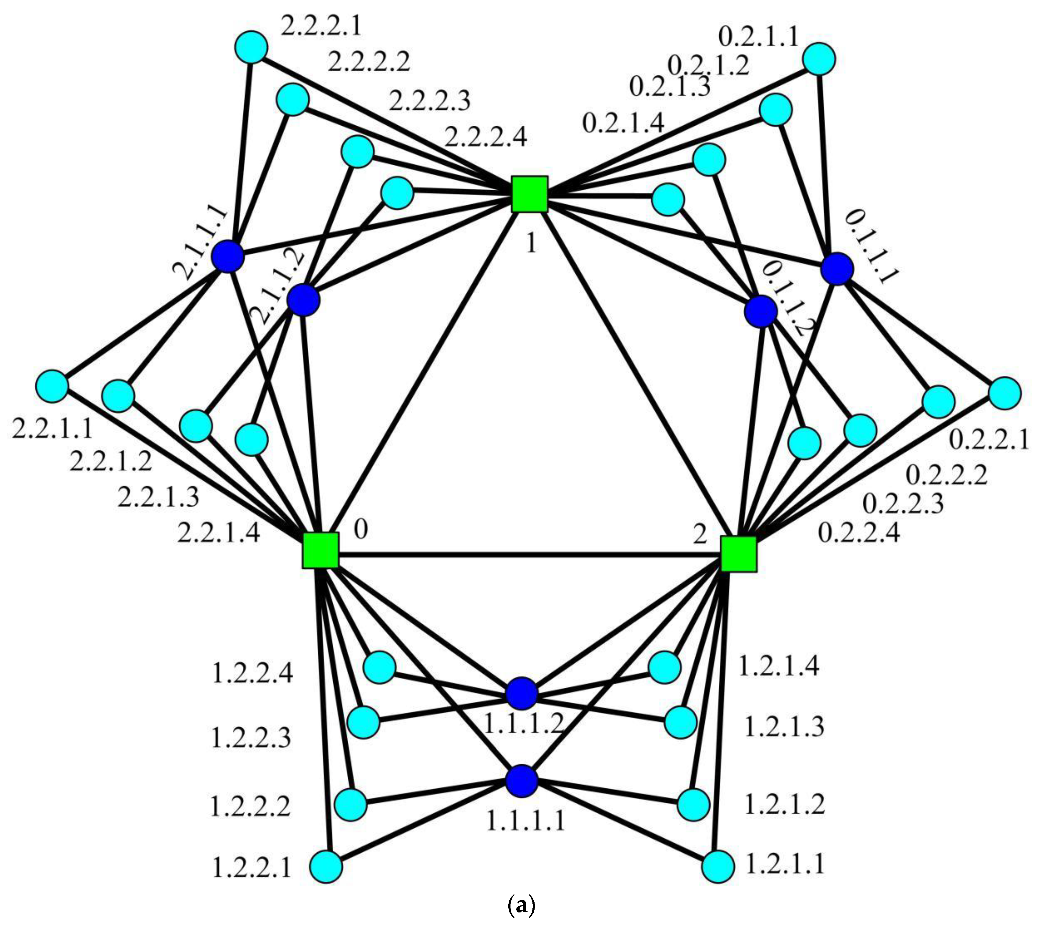
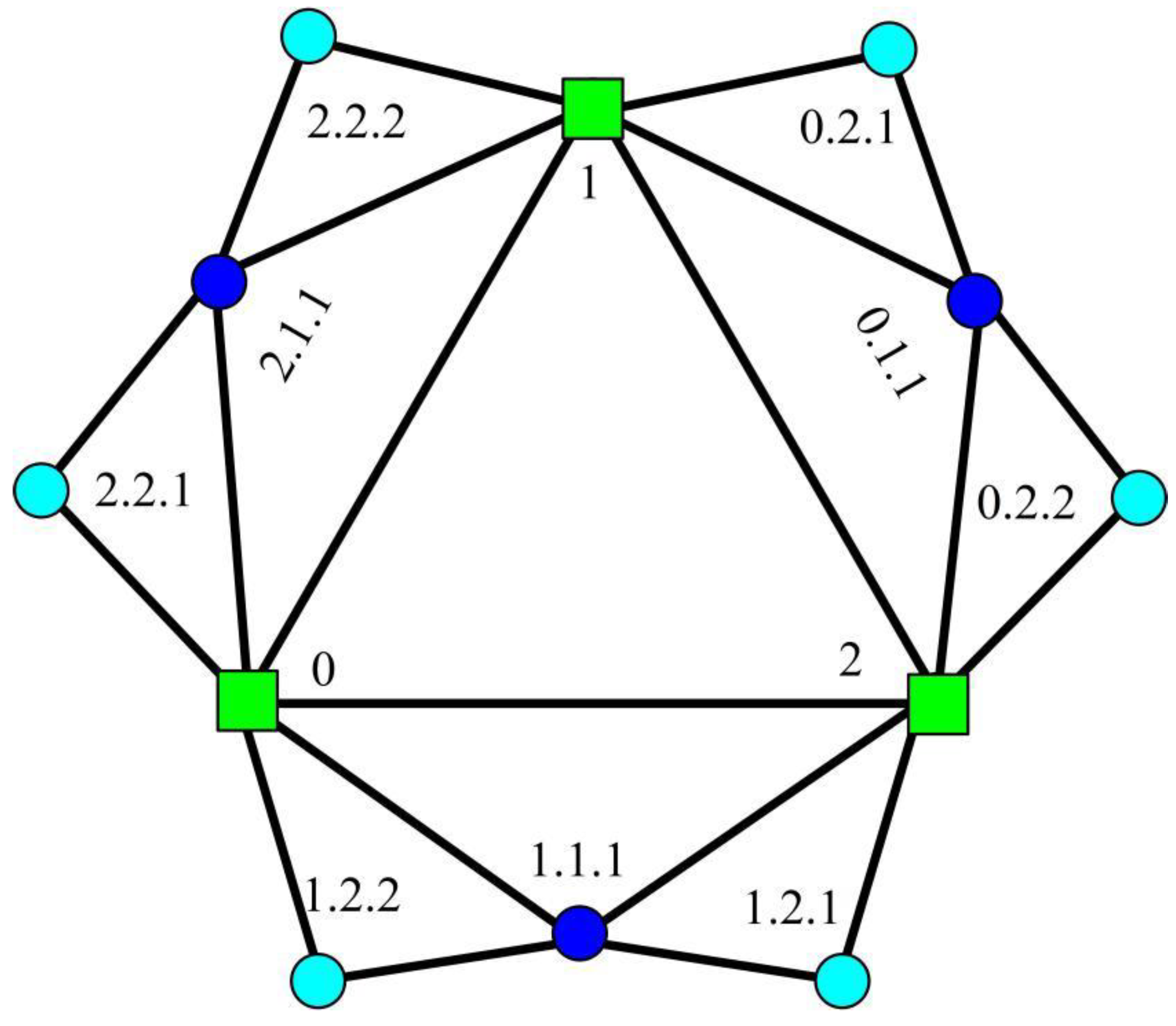
Definition 5.

(The labeling of GFG) The labeling of any vertex in $GF(t,k)$ adheres to the following rules:

• The three initial vertices are labeled with 0, 1 and 2.
• At any step$t\ge 1$, a vertex in$GF(t,k)$is marked with$a.b.c.d$according to the group ($a$), the subgroup ($b.c$) and the precise positions ($d$) from down to top in the same subgroup, in which$a\in \{0,1,2\}$,$b=\{1,2,\dots ,t\}$,$c\in \{1,2,\dots ,2^{b-1}\}$and$d\in \{1,2,\dots ,k^b\}$.

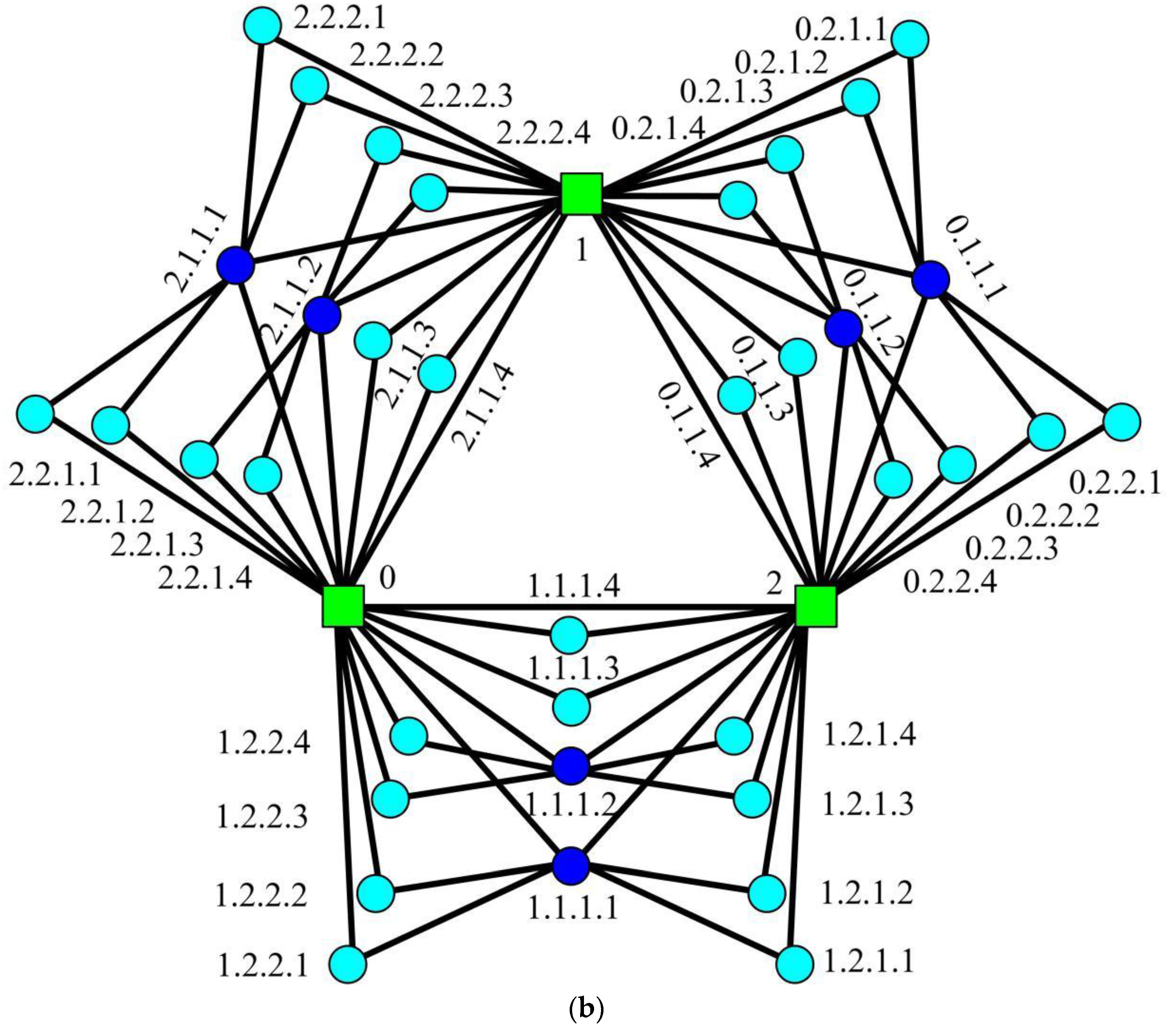
Definition 6.

(The labeling of EFG) Vertices in$EF(t,k)$are labeled as follows:

• Label three initial vertices as 0, 1 and 2.
• At step$t\ge 1$, a vertex is tagged with$a.b.c.d$, in which$a\in \{0,1,2\}$,$b=\{1,2,\dots ,t\}$,$c\in \{1,2,\dots ,$$2^{b-1}\}$and$d\in \{1,2,\dots ,(t-b+1)\times k^b\}$.

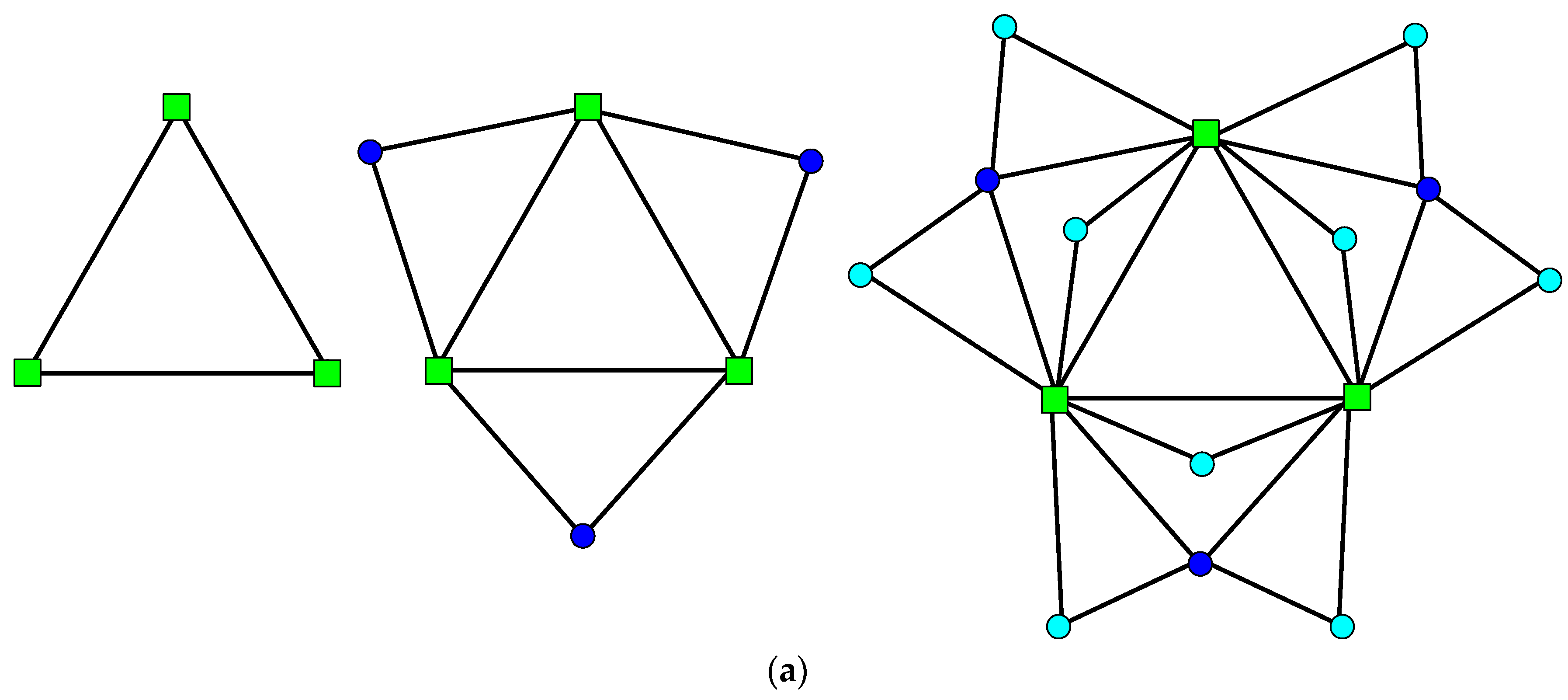
Labeling of$GF(2,2)$and$EF(2,2)$are illustrated in Figure 6.

Remark 4.

A GFG has more petals than an EFG, such that$d_{\max }=(t-b+1)\times k^b$in EFG, while$d_{\max }=k^b$in GFG.

When $t\ge 2$, any new vertex, added to GFG/EFG at step $t_i$, links to two vertices: a mother and a father. The vertices added to graphs at the same time are siblings if they have the same parents. Supposing that two arbitrary vertices in GFG/EFG are labeled with $a_1.b_1.c_1.d_1$ and $a_2.b_2.c_2.d_2$, in which $b_1\ge b_2$, then, we give several properties satisfying GFG and EFG at once.

Property 7.

(The family of $a.b.c.d$)

When$b\ge 1$,$a.b.c.d$belongs to a set of siblings {$a.b.c.(k\lfloor \frac{d}{k}\rfloor +1),a.b.c.(k\lfloor \frac{d}{k}\rfloor +2)$, $\dots ,a.b.c.(k\lfloor \frac{d}{k}\rfloor +k)$}.

When$b\ge 2$,$a.b.c.d$and its parents define a triangle, the mother is$a.(b-1).\lfloor \frac{c}{2}\rfloor .\lfloor \frac{d}{k}\rfloor$, the father is$a.(b-l).\lfloor \frac{c-rem(c,2)}{2^l}\rfloor .\lfloor \frac{d}{k^l}\rfloor$.

If$b\ge b_0$, the$(b-b_0)th$generation of maternal ancestor of$a.b.c.d$is$a.b_0.\lfloor \frac{c}{2^{b-b_0}}\rfloor .\lfloor \frac{d}{k^{b-b_0}}\rfloor$.

Proof. 

The above results are self-evident, with the exception of the formulation of the father’s label, which we shall now prove. If $b\ge 2$, let $l$ denotes the difference $b-b_1$, thus, $l\in \{2,\dots ,b-2\}$. When $c=1$ and with any $b$, the fathers are all the initial vertexes. When $c$ is odd but excluding one, $l$ is one plus the number of the continuous zeros from right to left in the binary representation of $c-1$, such that the father is labeled as $a.(b-l).\lfloor \frac{c-1}{2^l}\rfloor .\lfloor \frac{d}{k^l}\rfloor$. When $c$ is even, the time difference $l$ is one plus the number of the continuous zeros from right to left of the binary representation of $c$, such that the father’s label is $a.(b-l).\lfloor \frac{c}{2^l}\rfloor .\lfloor \frac{d}{k^l}\rfloor$. In summary, the father of $a.b.c.d$ is $a.(b-l).\lfloor \frac{c-rem(c,2)}{2^l}\rfloor .\lfloor \frac{d}{k^l}\rfloor$ when $b\ge 2$. ☐

Remark 5.

The vertex$a\mathrm{.1.1.}d$has two mothers$\{0,1,2\}/\left\{a\right\}$and no father. The three initial vertices have no parents or siblings. Therefore, the neighbors of$a.b.c.d$are derived from Property 8.

Property 8.

(The neighbors of $a.b.c.d$)

When$b\ge 2$, the set of neighbors of$a.b.c.d$is$\{a.(b-l).\lfloor \frac{c-rem(c,2)}{2^l}\rfloor .\lfloor \frac{d}{k^l}\rfloor ,a.(b-1).\lfloor \frac{c}{2}\rfloor .\lfloor \frac{d}{k}\rfloor$,$a.(b+x){.2}^{x-1}(2c-1).d$,$a.(b+x).[2^{x-1}(2c-1)+1].d\}$, in which$x\in \{1,2,\dots ,t-b\}$,$d\in \{(b+x-1)\times k^x$$+1,(b+x-1)\times k^x+2,\dots ,(b+x)\times k^x\}$.

The neighbors of initial vertex$a$are$\{0,1,2\}/\left\{a\right\}\cup \{a.b\mathrm{.1.}d\}\cup \{a.b{.2}^{b-1}.d\}$, where$b\in \{1,2,\dots ,$$t\}$,$d\in \{1,2,\dots ,k^b\}$.

The neighbors of$a\mathrm{.1.1.}d$are$\{0,1,2\}/\left\{a\right\}$and$\{a.(1+x){.2}^{x-1}.d,a.(1+x).(2^{x-1}+1).d\}$, where$x\in \{1,2,\dots ,t-1\}$,$d\in \{(b+x-1)\times k^x+1,(b+x-1)$$\times k^x+2,\dots ,(b+x)\times k^x\}$.

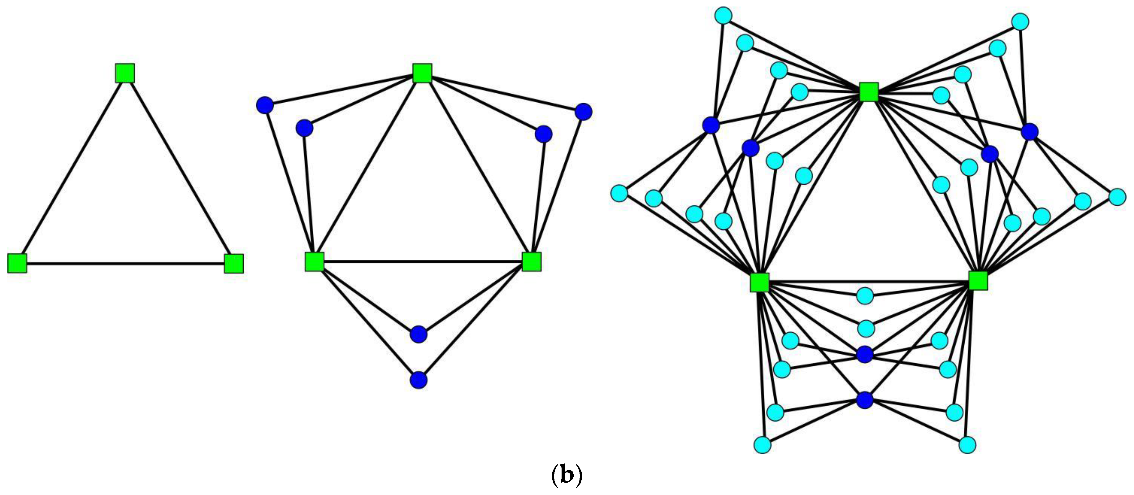
Property 9.

(The projection of GFG/EFG) By merging vertices$a.b.c.d$, which have the same$a.b.c$but a different$d$, into a vertex labeling with$a.b.c$,$GF(t,k)$/$EF(t,k)$is projected onto a graph which is exactly the combination of three Farey graphs starting from each edge of a triangle.

Proof. 

From the spatial relationship between vertices in different petals, all the vertices of $a\mathrm{.1.1.}d$ are linked to common vertices up until two initial vertices $\{0,1,2\}/\left\{a\right\}$ are reached, so that all of $a\mathrm{.1.1.}d$ can merged into a vertex of $a\mathrm{.1.1}$. By recursively using the spatial relationship, $GF(t,k)$/$EF(t,k)$ is projected into a combination of three Farey graphs. ☐

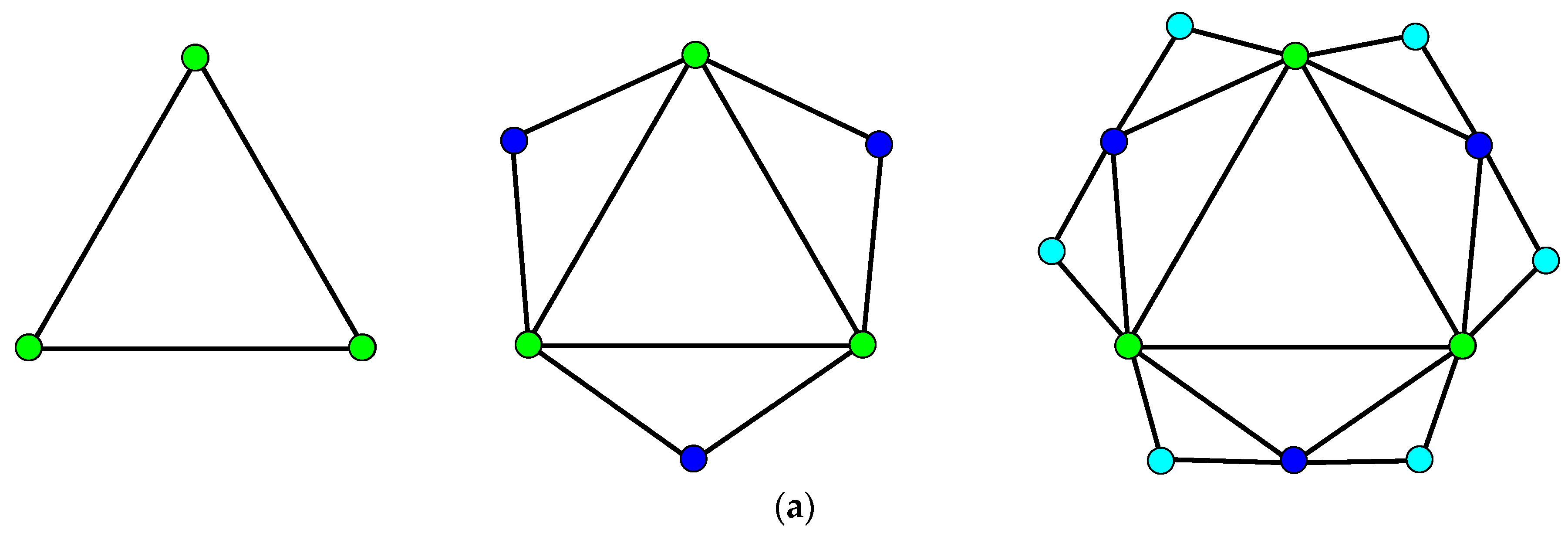
Example 1.

The projection graph of$GF(2,2)$/$EF(2,2)$is shown as Figure 7.

Property 10.

(The slice defined by $a.b.c.d$) For any vertex$a.b.c.d$, the slice is obtained by recursively identifying all triangles, which are shaped by a vertex and its parents, up until two initial vertices are reached.

Proof. 

Any vertex $a.b.c.d$ has a father $a.(b-l).\lfloor \frac{c-rem(c,2)}{2^l}\rfloor .\lfloor \frac{d}{k^l}\rfloor$ and a mother $a.(b-1).$ $\lfloor \frac{c}{2}\rfloor .\lfloor \frac{d}{k}\rfloor$ by Property 7, and the three vertices define a triangle. Then, the father’s mother, or the mother’s father, is obtained by recursively using Property 7. From the spatial relationship of vertices, $a.b.c.d$ and all these parents define a slice. ☐

5. Routing of $GF(t,k)$ and $EF(t,k)$

Although the labels of the three initial vertices in GFG and EFG are slightly different from the labels of the two initial vertices in FG, the shortest paths protocol in GFG/EFG also benefit from the routing algorithm in FG. From the generation mechanism, GFG/EFG is divided into three groups by symmetry, and each group is consisted of $k$ or $t\times k$ petals, and furthermore vertices in each group can also be divided into three sets by the differences in distance, similar to the equivalent division for FG: sets $V_{}^x(t)$, $V_{}^{xy}(t)$ and $V_{}^y(t)$.

Property 11.

(The characteristic of shortest paths when two vertices are located in different groups)

If$a_1\ne a_2$, the initial vertex$\{0,1,2\}/\{a_1,a_2\}$is on the shortest paths between$a_1.b_1.c_1.d_1$and$a_2.b_2.c_2.d_2$of GFG/EFG, if

(a)$a_1.b_1.c_1\in V_1^x(t)\cup V_1^{xy}(t)$and$a_2.b_2.c_2\in V_2^x(t)\cup V_2^{xy}(t)$,

(b) or$a_1.b_1.c_1\in V_2^x(t)\cup V_2^{xy}(t)$and$a_2.b_2.c_2\in V_1^x(t)\cup V_1^{xy}(t)$,

(c) or$a_1.b_1.c_1\in V_1^x(t)$and$a_2.b_2.c_2\in V_2^y(t)/\left\{a_2\right\}$,

(d) or$a_1.b_1.c_1\in V_2^x(t)$and$a_2.b_2.c_2\in V_1^y(t)/\left\{a_1\right\}$.

The two initial vertices$a_1$and$a_2$are on the shortest paths, if

(a)$a_1.b_1.c_1\in V_1^y(t)$and$a_2.b_2.c_2\in V_2^y(t)$,

(b) or$a_1.b_1.c_1\in V_2^y(t)$and$a_2.b_2.c_2\in V_1^y(t)$.

The shortest paths pass$\{0,1,2\}/\{a_1,a_2\}$,$a_1$and$a_2$simultaneously, if

(a)$a_1.b_1.c_1\in V_1^y(t)$and$a_2.b_2.c_2\in V_2^{xy}(t)$,

(b) or$a_1.b_1.c_1\in V_2^y(t)$and$a_2.b_2.c_2\in V_1^{xy}(t)$.

Proof. 

From Property 9, $a_1.b_1.c_1.d_1$ and $a_2.b_2.c_2.d_2$ are projected as $a_1.b_1.c_1$ and $a_2.b_2.c_2$, which are located in different subgraphs $F_1(t)$ and $F_2(t)$ of Farey graphs $F(t+1)$. Following from the proof of Property 3, the conclusions can easily be deduced. ☐

Property 12.

(The characteristic of shortest paths when two vertices lie in different slices of same group) If$a.b_1.c_1.d_1$and$a.b_2.c_2.d_2$are located in different petals, the shortest paths between them are positioned in two slices which are connected by two common vertices.

Proof. 

From the generating algorithm, if $a.b_1.c_1.d_1$ and $a.b_2.c_2.d_2$ are located in different petals or subpetals, then the neighbor sets of $a.b_1.c_1.d_1$ and $a.b_2.c_2.d_2$ are ascertained by Property 8. When two common neighbors are created during the same step, then $a.b_1.c_1.d_1$ and $a.b_2.c_2.d_2$ are positioned in different slices, and the two slices can be determined by Property 10. Supposing that the first two common neighbors are $a.b_3.c_3.d_3$ and $a.(b_3+1).c_4.d_4$, the two slices are rooted in them and belong to $F(b_1-b_3)$ and $F(b_2-b_3)$. 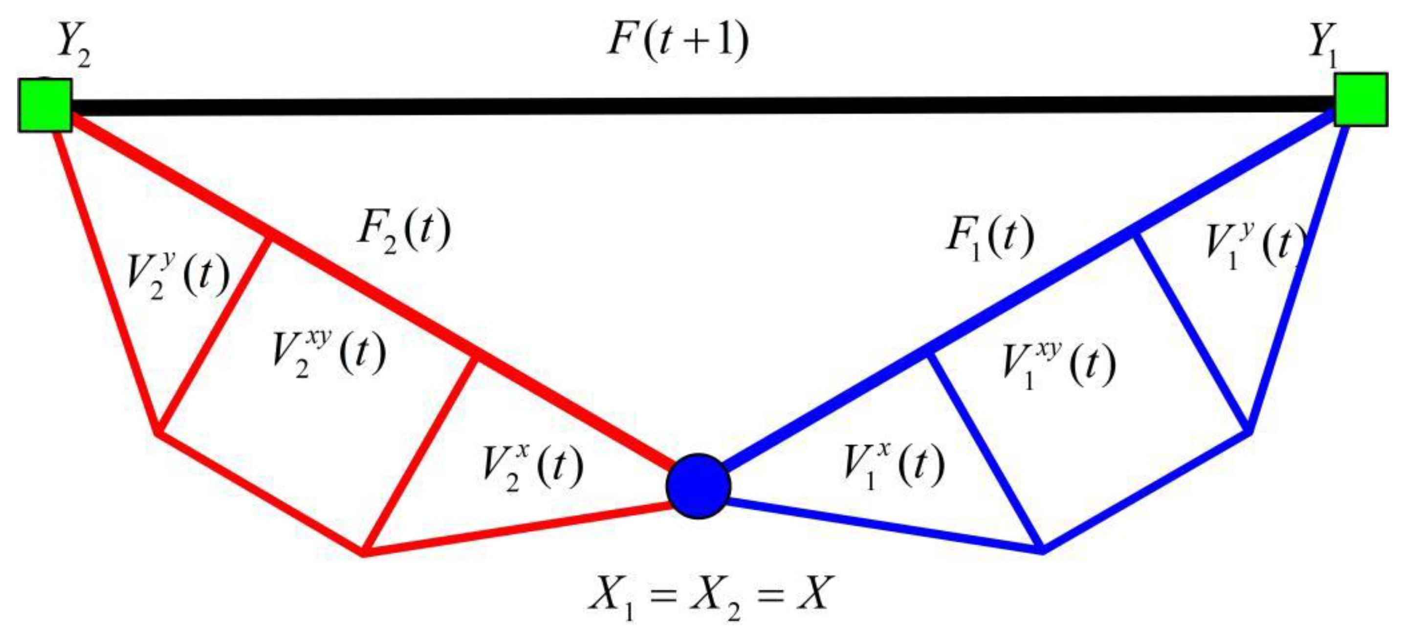Compared with the construction schematic diagram in Figure 2, the linking of $F(b_1-b_3)$ and $F(b_2-b_3)$ is slightly different. Name the initial vertices of $F(b_1-b_3)$ and $F(b_2-b_3)$ as $X_1$, $X_2$ and $Y_1$, $Y_2$, respectively. $F(b_1-b_3)$ and $F(b_2-b_3)$ are linked exactly by merging $X_1$ and $Y_1$ into $a.b_3.c_3.d_3$ and linking $X_2$ and $Y_2$ into $a.(b_3+1).c_4.d_4$. The vertices of $F(b_1-b_3)$ and $F(b_2-b_3)$ can be divided into six parts similarly: $V_{\alpha }^x(t)$, $V_{\alpha }^{xy}(t)$, $V_{\alpha }^y(t)$ and $V_{\beta }^x(t)$, $V_{\beta }^{xy}(t)$, $V_{\beta }^y(t)$, by the distance between $a.b_1.c_1.d_1$ or $a.b_2.c_2.d_2$ to initial vertices $X$ (i.e., $a.b_3.c_3.d_3$) and $Y$ (i.e., $a.(b_3+1).c_4.d_4$), in which case then the shortest paths between $a.b_1.c_1.d_1$ and $a.b_2.c_2.d_2$ go via $a.b_3.c_3.d_3$, if

(a) $a.b_1.c_1\in V_{\alpha }^x(t)$ and $a.b_2.c_2\in V_{\beta }^x(t)$,

(b) $a.b_1.c_1\in V_{\alpha }^x(t)$ and $a.b_2.c_2\in V_{\beta }^{xy}(t)$,

(c) or $a.b_1.c_1\in V_{\alpha }^{xy}(t)$ and $a.b_2.c_2\in V_{\beta }^x(t)$.

The shortest paths go through $a.b_3.c_3.d_3$ and $a.(b_3+1).c_4.d_4$, if

(a) $a.b_1.c_1\in V_{\alpha }^x(t)$ and $a.b_2.c_2\in V_{\beta }^y(t)$,

(b) or $a.b_1.c_1\in V_{\alpha }^{xy}(t)$ and $a.b_2.c_2\in V_{\beta }^{xy}(t)$,

(c) $a.b_1.c_1\in V_{\alpha }^y(t)$ and $a.b_2.c_2\in V_{\beta }^x(t)$.

The shortest paths pass $a.(b_3+1).c_4.d_4$, if

(a) $a.b_1.c_1\in V_{\alpha }^{xy}(t)$ and $a.b_2.c_2\in V_{\beta }^y(t)$,

(b) $a.b_1.c_1\in V_{\alpha }^y(t)$ and $a.b_2.c_2\in V_{\beta }^{xy}(t)$,

(c) or $a.b_1.c_1\in V_{\alpha }^y(t)$ and $a.b_2.c_2\in V_{\beta }^y(t)$. ☐

Property 13.

(The characteristic of shortest paths when two vertices are in same slice) If$a.b_1.c_1.d_1$and$a.b_2.c_2.d_2$are in the same slice of a petal or subpetal of same group, the shortest paths between them are determined by Property 5, as they have been projected onto a Farey graph.

Proof. 

If we obtained only one common neighbor vertex, labeled with $a.b_3.c_3.d_3$, of vertices $a.b_1.c_1.d_1$ and $a.b_2.c_2.d_2$ at the same step, then $a.b_1.c_1.d_1$ and $a.b_2.c_2.d_2$ are located in same slice. Assuming $b_1\ge b_2$, the projected Farey graph is $F(b_1-b_3-1)$ with a hub vertex $a.b_1.c_1.d_1$, in which case all the shortest paths are located in $F(b_1-b_3-1)$. So that all the shortest paths can be decided by Property 5. ☐

The detailed shortest routing algorithm in GFG/EFG is described as follows.

Property 14.

(The shortest paths routing algorithm in GFG/EFG)

1. Given any two vertices$a_1.b_1.c_1.d_1$and$a_2.b_2.c_2.d_2$, insert$a_1.b_1.c_1.d_1$and$a_2.b_2.c_2.d_2$into the labels set of the shortest paths ($LSS{P}_m(h)$), $LSS{P}_m(0)=\varnothing$.

2. If$a_1\ne a_2$, and both$a_1.b_1.c_1.d_1$and$a_2.b_2.c_2.d_2$are not initial vertices, then this is exactly the condition of two vertices being in different groups. Three initial vertices$\{0,1,2\}/\{a_1,a_2\}$,$a_1$and$a_2$are ascertained as being on the shortest paths or not by property 11.

If only$\{0,1,2\}/\{a_1,a_2\}$is on the paths, insert the label$\{0,1,2\}/\{a_1,a_2\}$in the middle of$a_1.b_1.c_1.d_1$and$a_2.b_2.c_2.d_2$in$LSS{P}_m(h)$,$h=h+1$, and generate two new pairs of labels:$a_1.b_1.c_1.d_1$and$\{0,1,2\}/\{a_1,a_2\}$,$\{0,1,2\}/\{a_1,a_2\}$and$a_2.b_2.c_2.d_2$, respectively.

If only$a_1$and$a_2$are on the paths, insert the labels$a_1$and$a_2$in the middle of two labels$a_1.b_1.c_1.d_1$and$a_2.b_2.c_2.d_2$,$h=h+2$, and get two new pairs of labels:$a_1.b_1.c_1.d_1$and$a_1$,$a_2$and$a_2.b_2.c_2.d_2$.

If$\{0,1,2\}/\{a_1,a_2\}$,$a_1$and$a_2$are all on the paths, combine the two conditions above together.

Go back to step 1 with the new label pairs.

3. If$a_1\ne a_2$, and$a_1.b_1.c_1.d_1$or$a_2.b_2.c_2.d_2$is an initial vertex, then it is the case of two vertices located in the same slice of a petal or subpetal in the same group. The common Farey graphs$F(b_1)$or$F(b_2)$are obtained by Property 13, in which case the shortest paths can be deduced by Property 5.

4. If$a_1=a_2=a$and$a.b_1.c_1.d_1$and$a.b_2.c_2.d_2$are not initial vertices, find out the neighbors of$a.b_1.c_1.d_1$and$a.b_2.c_2.d_2$by Property 8.

If two common neighbors are obtained at the same step, then$a.b_1.c_1.d_1$and$a.b_2.c_2.d_2$are located in different slices. Whether the two common neighbors are positioned on the shortest paths or not are determined by Property 3. Assuming two common neighbors are$a.b_3.c_3.d_3$and$a.b_4.c_4.d_4$, if$a.b_3.c_3.d_3$(or$a.b_4.c_4.d_4$) is on the shortest paths, insert the label$a.b_3.c_3.d_3$(or$a.b_4.c_4.d_4$) in the middle of$a_1.b_1.c_1.d_1$and$a_2.b_2.c_2.d_2$,$h=h+1$, and generate two new pair labels of$a_1.b_1.c_1.d_1$and$a.b_3.c_3.d_3$(or$a.b_4.c_4.d_4$), and$a.b_3.c_3.d_3$(or$a.b_4.c_4.d_4$) and$a_2.b_2.c_2.d_2$. If$a.b_3.c_3.d_3$and$a.b_4.c_4.d_4$are both on the shortest paths at the same time, insert the label$a.b_3.c_3.d_3$and$a.b_4.c_4.d_4$in the set$LSS{P}_m(h)$,$h=h+1$,$m=m+1$, and make up four new pair labels of$a_1.b_1.c_1.d_1$and$a.b_3.c_3.d_3$,$a_1.b_1.c_1.d_1$and$a.b_4.c_4.d_4$,$a.b_3.c_3.d_3$or$a_2.b_2.c_2.d_2$,$a.b_4.c_4.d_4$and$a_2.b_2.c_2.d_2$. Go back to step 1 with the new label pairs.

If only one common neighbor is obtained at the same time, then$a.b_1.c_1.d_1$and$a.b_2.c_2.d_2$are located in same slice. The shortest paths are projected into a Farey graph, and then all the shortest paths are derived by Property 5.

Remark 6.

The expanded deterministic Apollonian networks, denoted by$A(d,t)$, are the generalization of Apollonian networks, being simultaneously small-world, scale-free and highly clustered. The label-based routing protocol for it is deduced in [35].$A(d,t)$($d\ge 1$and$t\ge 0$) are constructed as follows.$A(d,0)$is a complete graph$K_{d+2}$(or$d+1$-clique).$A(d,t)$($t\ge 1$) is obtained from$A(d,t-1)$by adding one new node and connecting it to all the nodes of each existing subgraph of$A(d,t-1)$that is isomorphic to a (d + 1)-clique and created at step$t-1$. Apparently,$A(1,t)$is exactly the same as the special case of the generalization of Farey graphs$GF(t,1)$, however, the algorithm in [35] can only get one of shortest paths in it.

Recursive clique-trees,$K(q,t)$($q\ge 2$,$t\ge 0$), have scale-free and small-world properties and allow a fine tuning of the power-law exponent of their discrete degree distribution and clustering [38].$K(q,t)$is the graph constructed as follows:$K(q,0)$is the complete graph$K_q$(or q-clique).$K(q,t)$is obtained from$K(q,t-1)$by adding to each of its existing subgraphs isomorphic to a q-clique a new vertex and then joining it to all the vertices of the subgraph. From the construction mechanisms used,$K(2,t)$is the same as the extended Farey graphs $EF(t-1,1)$. Same as in Ref. [35], the protocol in [38] can only get one of shortest paths.

6. Conclusions

We presented label-based routing algorithms for Farey-type graphs, including standard Farey graphs, generalized Farey graphs and extended Farey graphs. Our results can be extended easily to several Farey-type deterministic models, such as models created by edge iteration, evolving graphs with general geometric growth models for pseudofractal scale-free webs, geographical attachment preference, graphs with multidimensional growth, and so on. In contrast with prior research results, which can only get one shortest path from the labels of any pair of vertices, we can ascertain all the shortest paths using only their labels in all Farey-type graphs.

As all Farey-type graphs are structurally isomorphic, the time complexity of the routing algorithm in generalized Farey graphs (GFG) and extended Farey graphs (EFG) are essentially equivalent to that of standard Farey graphs, and thus the routing algorithms run in logarithmic time O(logn).

For weighted scale-free small-world graphs [44] and delayed pseudofractal graphs [45], our solutions can also be easily extended to these weighted or delayed models.