Some Interacting Dark Energy Models

Abstract

In this paper, we study various cosmological models involving new nonlinear forms of interaction between cold dark matter (DM) and dark energy (DE) assuming that DE is a barotropic fluid. The interactions are nonlinear either due to $log({\rho }_{de}/{\rho }_{dm})$ or $log({\rho }_{dm}/{\rho }_{de})$ parameterizations, respectively. The main purpose of this paper is to demonstrate the applicability of the forms of suggested interactions to the problem of modern cosmology known as accelerated expansion of the Universe. Using the differential age of old galaxies expressed in terms of $H\left(z\right)$ data, the peak position of baryonic acoustic oscillations (known as BAO data), the SN Ia data with strong gravitational lensing data, we obtain the best fit values of the model parameters for each case. Besides, using $Om$ analysis and $S_3$ parameter from the statefinder hierarchy analysis, we also demonstrate that the considered models are clearly different from the $\mathsf{\Lambda }$CDM model. We obtain that the models predict Hubble parameter values consistent to the estimations from gravitational lensing, which probes the expansion out to $z\le 1.7$. We show that, with considered models, we can also explain PLANCK 2015 and PLANCK 2018 experiment results.

1. Introduction

It is well known that the standard cosmological model ($\mathsf{\Lambda }$CDM), where the cosmological constant plays the role of dark energy(DE), has two theoretical problems. These are very well know problems and one of them is the cosmological coincidence problem [1,2] (and references therein). It is very well known that the simple question encoded inside the cosmological coincidence problem can be answered using interacting DE and dark matter (DM) models. Therefore, one of the central ideas in modern cosmology is the interaction between DE and DM. It is obvious that using this idea also will provide an alternative option to explain the accelerated expansion of the low redshift Universe. The topic of interacting DE models is an often discussed topic in recent literature. On the other hand, according to General Relativity (GR), there is no restriction on the existence/form of interaction between other energy sources providing/contributing the background dynamics of our Universe. Nevertheless, it is not clear where interactions between two energy sources operating on different scales in our Universe can arise from, even though it can be useful to solve DE related problems, as has been mentioned above. Moreover, in particular, interaction also affects on the type and formation of finite-time future singularities. We can assume for a while that the origin of DE–DM interaction is related to emergence of the spacetime dynamics. However, this is not of much help, since this hypothesis is not more fundamental compared with other phenomenological assumptions within modern cosmology [3,4,5,6,7,8,9,10,11,12,13,14,15,16,17,18,19,20] (and references therein for an extended discussion on the points mentioned above). On the other hand, besides not well understood origin of DE–DM interaction, there is also another important questions related to the energy flow direction. In particular, in early literature, the energy flow from DE to DM has been considered, but latter developments demonstrated that the energy flow from DM to DE is also possible (see, for instance, [21] and other references of this paper).

The purpose of this paper is to develop cosmological models, where new phenomenological forms of interactions are involved. In particular, we study how new forms of interactions constructed in this paper help to solve the cosmological coincidence problem. Moreover, using constructed models, we also study the problem related to the Hubble constant tension [22,23,24]. Since we are interested mainly in the problem of the accelerated expansion of the low redshift Universe, we follow the well known approximation of the energy content of the recent Universe (for details, we refer the reader to [25] and references therein). Namely, we consider cold DM and barotropic dark fluid with negative constant equation of state parameter to represent the effective fluid with

$$P_{eff}=P_{de}={\omega }_{de}{\rho }_{de},$$

(1)

and

$${\rho }_{eff}={\rho }_{de}+{\rho }_{dm}.$$

(2)

The need to have DE to provide correct background dynamics consistent with the observational data is a well known fact and we refer the readers to [25] for more details on this issue. The presentation of DE as a barotropic fluid with constant equation of state parameter is one of the simplest ways considered in the recent literature. In general, there are various ways to present DE and one of them is the scalar field representation giving various interesting options. The other possibilities are the parameterization of either the energy density or the pressure of DE. In particular, holographic and ghost DE models are the models given by the parameterization of the energy density. On the other hand, an interesting approach to represent DE can be associated to Chaplygin gas [13] and van der Waals fluid [19]. These are examples of how DE can be interpreted as dark fluid. The existence and variety of DE models are directly associated with the fact that the tension between different datasets does not allow choosing one of them as the best candidate [26] (and references therein). However, the simplest model for DE is still the cosmological constant with equation of state parameter $-1$. On the other hand, as we mentioned above, with this model, we have additional problems, which can be solved with dynamical DE models, such as ghost dark energy, holographic dark energy and generalized holographic dark energy with Nojiri–Odintsov cut-off to mention a few [21,27,28,29,30,31,32,33,34,35,36,37,38]. There is a systematic update in DE interpretation as dark fluid and one of them is the varying polytropic fluid presented in Reference [34] (see the references therein about other models of dark fluids). With the accelerated expansion of the Universe, DE and DM problems can also be explained by modifying GR [39,40,41,42,43,44,45,46,47,48,49,50,51,52,53,54,55]. On the other hand, it can be done by particle creation, which generates negative pressure [56,57,58,59,60] (to mention a few).

The main approach to be convinced on the viability of suggested cosmological scenario is to compare the theoretical results with observational data. In general, a model can be constrained using the background tests and the growth test. In this work, we concentrate our attention only on the background tests involving the following four datasets (see, for instance, [61] and references therein for more details about the used datasets):

• The differential age of old galaxies, given by $H\left(z\right)$.
• The peak position of baryonic acoustic oscillations (BAO).
• The SN Ia data.
• Strong Gravitation Lensing data.

In the case of the Observed Hubble Data, one defines chi-square given by

$${\chi }_{OHD}^2=\sum \frac{{\left(H(\mathbf{P},z)-H_{obs}\left(z\right)\right)}^2}{{\sigma }_{OHD}^2},$$

(3)

where $H_{obs}\left(z\right)$ is the observed Hubble parameter at redshift z and ${\sigma }_{OHD}$ is the error associated with that particular observation, while $H(\mathbf{P},z)$ is the Hubble parameter obtained from the model and $\mathbf{P}$ is the set of the parameters to be determined/constrained from the dataset. On the other hand, seven measurements have been jointly used determining the BAO (Baryon Acoustic Oscillation) peak parameter to constrain the models by

$${\chi }_{BAO}^2=\sum \frac{{\left(A(\mathbf{P},z)-A_{obs}\left(z\right)\right)}^2}{{\sigma }_{BAO}^2},$$

(4)

where the theoretical value for the $\mathbf{P}$ set of the parameters $A(\mathbf{P},z)$ is determined as

$$A(\mathbf{P},z_1)=\frac{\sqrt{{\mathsf{\Omega }}_m}}{E{\left(z_1\right)}^{1/3}}{\left(\frac{{\int }_0^{z_1}\frac{dz}{E\left(z\right)}}{z_1}\right)}^{2/3},$$

(5)

with $E\left(z\right)=H\left(z\right)/H_0$ and $H_0$ the values of the Hubble parameter at $z=0$. For the Supernovae Data, ${\chi }_{\mu }^2$ is defined as

$${\chi }_{\mu }^2=A-\frac{B^2}{C},$$

(6)

where

$$A=\sum \frac{{(\mu (\mathbf{P},z)-{\mu }_{obs})}^2}{{\sigma }_{\mu }^2},$$

(7)

$$B=\sum \frac{\mu (\mathbf{P},z)-{\mu }_{obs}}{{\sigma }_{\mu }^2},$$

(8)

and

$$C=\sum \frac{1}{{\sigma }_{\mu }^2}.$$

(9)

In the last three equations, ${\sigma }_{\mu }$ is the uncertainty in the distance modulus [61].

If the analysis is carried out by including the Strong Gravitational Lensing data, we must follow to the receipt of Reference [62] and use data identical to the data presented there. The receipt of Reference [62] allows imposing observational constraints on the parameters of the models, without considering the structure and physics of the lensing object. To obtain appropriate constraints, usually known as the best fit values, of the parameters of the model, one needs to minimize ${\chi }^2$ function

$${\chi }^2={\chi }_{OHD}^2+{\chi }_{BAO}^2+{\chi }_{\mu }^2+{\chi }_{SGL}^2,$$

(10)

when all datasets are used simultaneously (for each combination of the datasets, appropriate total ${\chi }^2$ should be considered). The set of the parameters to be constrained by ${\chi }^2$ analysis for each model of this paper are presented in the next section during the discussion of the models.

The paper is organized as follows: in Section 2, we discuss the models and perform the analysis to demonstrate their viability. At the same time, we apply the well known ${\chi }^2$ statistical analysis to constraint the models. In this paper, we have a simple grid walk to seek the set of the parameters to minimize ${\chi }^2$. On the other hand, in Section 3 and Section 4, the analysis of two families of interacting DE and DM models has been performed and the results are discussed taking into account only the best fit values of the parameters obtained during the fit. The description of the models also includes a presentation of the forms of non-linear DE–DM interactions. In Section 5, we organize discussion on obtained results and present possible extensions of the models considered in this work.

2. Models and Observational Constraints

For the models considered in this paper, we assume that GR describes the background dynamics. Moreover, we consider a flat low redshift Universe with FRW metric and interacting dark components, for which the field equations read as

$$H^2=\frac{{\dot{a}}^2}{a^2}=\frac{\rho }{3},$$

(11)

$$\frac{\ddot{a}}{a}=-\frac{1}{6}(\rho +3P).$$

(12)

If we additionally assume that the effective fluid is ideal, we derive the following equations describing the dynamics of cold DM and DE (see, for instance, [29,63]):

$${\dot{\rho }}_{dm}+3H{\rho }_{dm}=Q,$$

(13)

$${\dot{\rho }}_{de}+3H{\rho }_{de}(1+{\omega }_{de})=-Q.$$

(14)

These equations describe interacting DE and DM models providing a transition from DE to DM, while ${\omega }_{de}$ is a negative constant (equation of state parameter of DE). It should be mentioned that, in this paper, we consider $\rho ={\rho }_{de}+{\rho }_{dm}$ including baryons into ${\rho }_{dm}$. The analysis of the models very often are performed using $Om$ analysis [64]. It is well known that $Om$ analysis is a geometrical tool to study DE models involving the following parameter [64]:

$$Om=\frac{x^2-1}{{(1+z)}^3-1},$$

(15)

where $x=H/H_0$. Note that the $Om$ analysis has been generalized to the two point $Om$ analysis with

$$Om(z_2,z_1)=\frac{x{\left(z_2\right)}^2-x\left(z_1^2\right)}{{(1+z_2)}^2-{(1+z_1)}^2}.$$

(16)

Moreover, a slight modification of the two-point $Om$ ($Om{h}^2$) is suggested in Reference [65] and the estimated values of the two point $Om{h}^2$ for $z_1=0$, $z_2=0.57$ and $z_3=2.34$:

$$Om{h}^2(z_1;z_2)=0.124\pm 0.045,$$

$$Om{h}^2(z_1;z_3)=0.122\pm 0.01,$$

$$Om{h}^2(z_2;z_3)=0.122\pm 0.012,$$

(17)

In general, it can also be used to obtain constraints on the parameters of the models.

Recall that, for the $\mathsf{\Lambda }$CDM mode, $Om{h}^2=0.1426$. The $Om$ analysis is the simplest tool to study DE models, since it connects the Hubble parameter and the redshifts. For other tools, such as statefinder hierarchy analysis, we need to calculate higher order derivatives of the scale factor, which makes calculations costly and complicated. To simplify our discussion, we organize two sections discussing the main results obtained from the ${\chi }^2$ technique for used datasets presented in Section 1.

3. Model 1

For the first cosmological model considered in this paper, we assume that the form of the interaction between DE and DM reads as

$$Q=3Hb{\rho }_{de}log\left[\frac{{\rho }_{de}}{{\rho }_{dm}}\right],$$

(18)

where b is a constant and should be determined from the observational data. On the other hand, ${\rho }_{de}$ and ${\rho }_{dm}$ are the densities of DE and DM. Suggested form of the interaction is constructed from the classical interaction term $Q=3Hb{\rho }_{de}$ intensively considered in the literature. According to Equations (13) and (14), the form of the interaction in Equation (18) indicates an energy transition from DE to DM. On the other hand, the transition from DM to DE can be modeled by

$$Q=3Hb{\rho }_{de}log\left[\frac{{\rho }_{dm}}{{\rho }_{de}}\right].$$

(19)

3.1. Transition from Dark Energy to Dark Matter

Consideration of the interaction in Equation (18) provides a cosmological model (including the parameters from the other assumptions) with the following $\{H_0,{\mathsf{\Omega }}_{dm}^{\left(0\right)},\omega ,b\}$ parameters, where $\omega$ is the equation of state parameter of DE, while ${\mathsf{\Omega }}_{dm}^{\left(0\right)}={\rho }_{dm}^{\left(0\right)}/3H_0^2$ and satisfies the following constraint

$${\mathsf{\Omega }}_{dm}^{\left(0\right)}+{\mathsf{\Omega }}_{de}^{\left(0\right)}=1.$$

(20)

Consideration on only energy transition from DE and DM impose on the parameter b to be strictly positive. This prior constraint on the parameter b is taken into account to constrain the other parameters of the model using the datasets and described statistical ${\chi }^2$ analysis presented above. On the other hand, to reduce the number of parameters and the computational time, for ${\mathsf{\Omega }}_{dm}^{\left(0\right)}$, we consider values of $0.26$, $0.27$, and $0.28$. Results in the existing scientific literature analyze, for instance, prior constraints on $\omega$ and $H_0$ of $[-1.2,-0.3]$ and $[67.5,73.5]$, respectively. With such priors, we obtain the best fit of the model with observational data described above as follows: $\{70.57,0.26,-1.03,0.0\}$, $\{70.22,0.27,-0.99,0.062\}$ and $\{69.88,0.28,-0.97,0.105\}$ with ${\chi }^2=784.2$, ${\chi }^2=780.9$ and ${\chi }^2=779.6$, respectively.

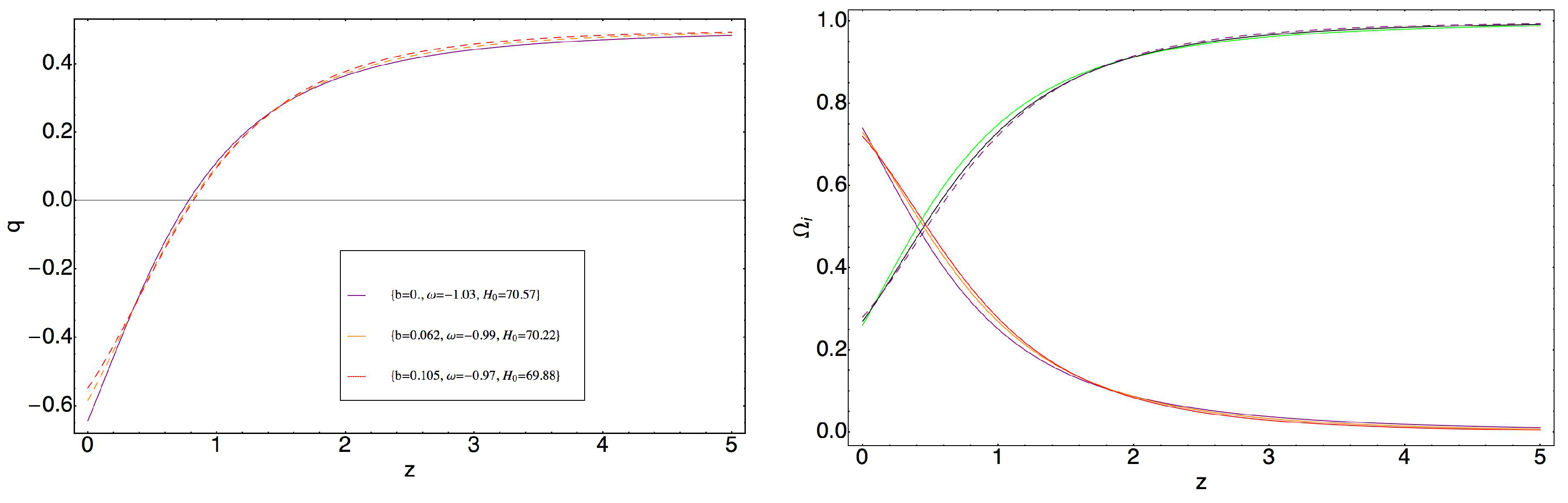
The graphical behavior of the deceleration parameter with the best fit values for the parameters is presented in Figure 1 (left). Transition between decelerated and accelerated expanding phases occurs. Moreover, the best fit results corresponding to ${\mathsf{\Omega }}_{dm}^{\left(0\right)}=0.27$ and ${\mathsf{\Omega }}_{dm}^{\left(0\right)}=0.28$ show a slightly earlier transition between mentioned expanding phases than the case with ${\mathsf{\Omega }}_{dm}^{\left(0\right)}=0.26$. On the other hand, since, for the parameter space scanning, we use the same priors and the same parameter space discretizing, we conclude that the model explains available/considered data (best fit with ${\chi }^2=779.6$) with $\{69.88,0.28,-0.97,0.105\}$. At the same time, Figure 1 (right) demonstrates that the model is free from the cosmological coincidence problem. The graphical behaviors of $Om$ and $S_3$ parameters representing $Om$ and statefinder hierarchy analysis (see [66] for the definition) are presented in Figure 2. We see clearly that both parameters are very sensitive on the values of the model parameters. Moreover, they indicate clear departures from the $\mathsf{\Lambda }$CDM model.

3.2. Transition from Dark Matter to Dark Energy

In this subsection, we discuss the results corresponding to the best fit for the cosmological model, where the interaction between DE and DM is given by Equation (19). According to the assumption about existence of the interaction between DE and DM, energy transfer from DM to DE is indicated, unlike the interaction given by Equation (18). During the study of this case, the prior constraint on the parameter b is extended. In particular, we allow b to be negative as well, which in this case also indicates transition from DE to DM corresponding to the case discussed in Section 3.1. In this case, $-0.99$, $-1.0$, $-1.02$, $-1.1$ and $-1.2$ discrete priors on $\omega$ are imposed and the following constraints $b=\{-0.095,-0.084,-0.062,0.24,0.3\}$, $H_0=\{69.86,69.76,69.65,69.35,70.68\}$ and ${\mathsf{\Omega }}_{dm}^{\left(0\right)}=\{0.28,0.28,0.28,0.28,0.28\}$ with ${\chi }^2=\{779.7,779.9,780.4,780.1,780.9\}$ are obtained.

From the obtained results, we see that, when DE is quintessence with allowed lower value for the equation of state parameter supported by PLANCK 2015 [67], the considered data support only energy transition from DE to DM, since $b<0$ in Equation (19). However, if with the parotropic fluid equation we attempt to obtain a phantom DE Universe, then it is possible only if transition for the energy will be from DM to DE, i.e., $b>0$. The graphical behaviors of the deceleration parameter q, ${\mathsf{\Omega }}_{de}$, ${\mathsf{\Omega }}_{dm}$ are presented in Figure 3. The graphical behaviors of $Om$ and $S_3$ parameters are presented in Figure 4.

4. Model 2

In this section, we present our study on the cosmological model, where the interaction between DE and DM is given by the following expression:

$$Q=3Hb{\rho }_{dm}log\left[\frac{{\rho }_{de}}{{\rho }_{dm}}\right].$$

(21)

Moreover, such interaction in our case leads to energy transition from DE to DM, while the interaction

$$Q=3Hb{\rho }_{dm}log\left[\frac{{\rho }_{dm}}{{\rho }_{de}}\right],$$

(22)

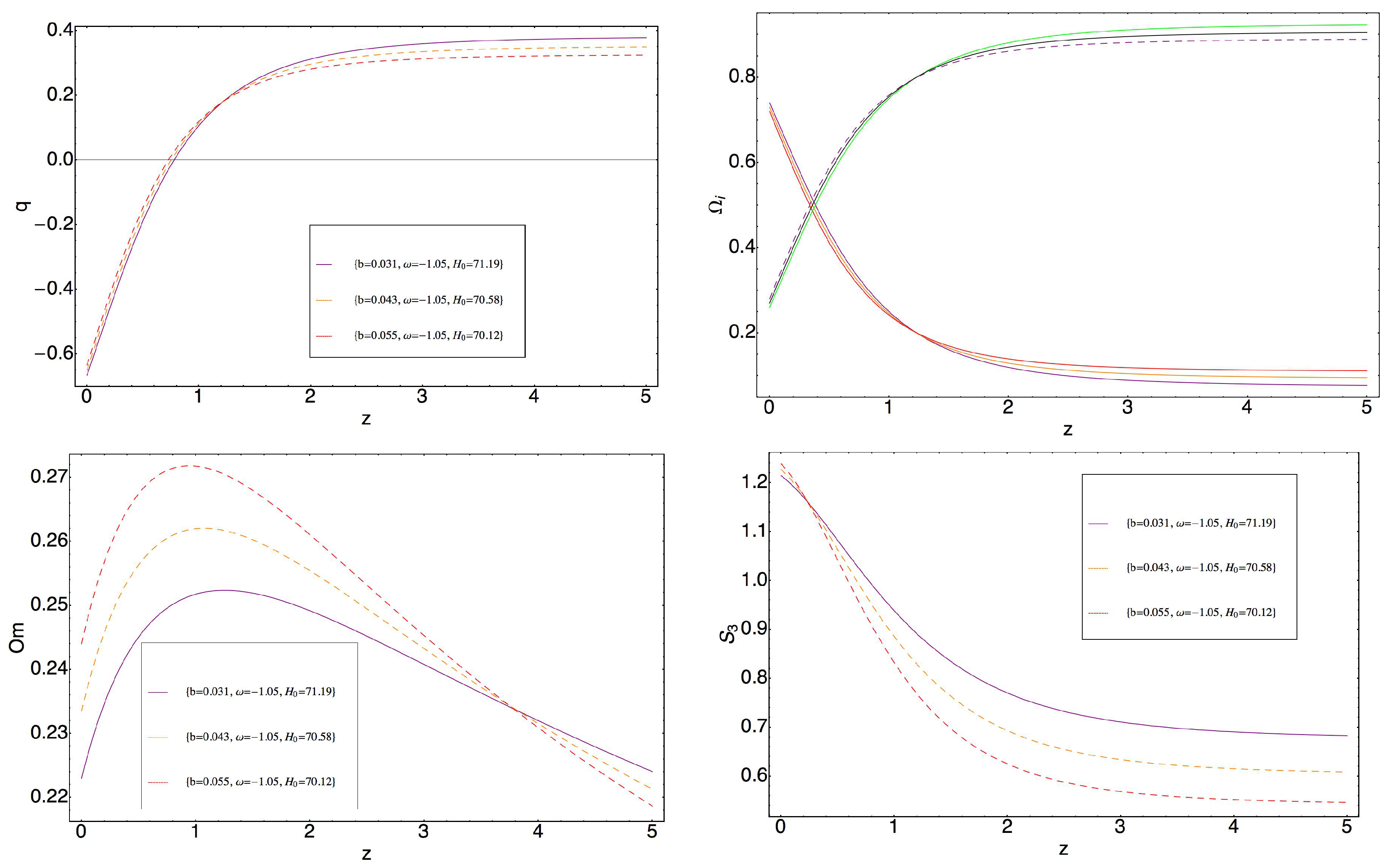
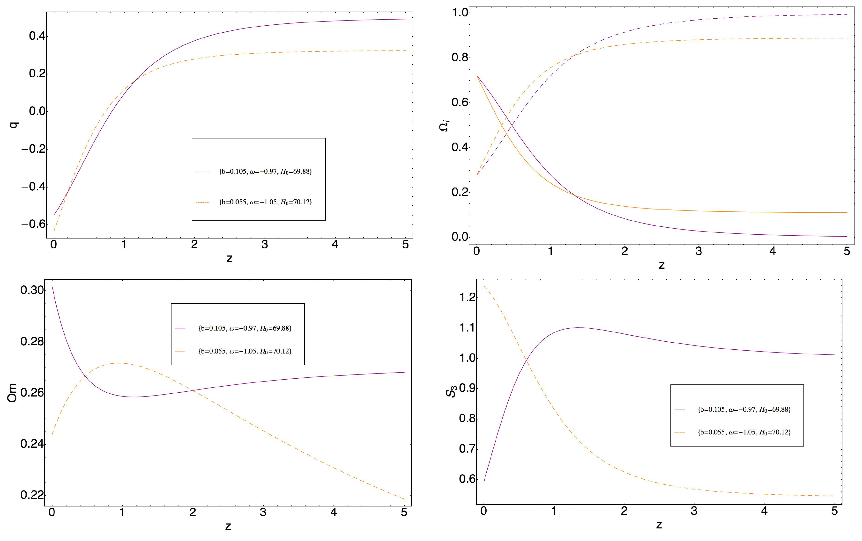
will indicate energy transition from DM to DE. In this case, the analysis reveals an interesting fact. Using ${\chi }^2={\chi }_{OHD}^2+{\chi }_{BAO}^2+{\chi }_{\mu }^2+{\chi }_{SGL}^2$ statistical technique, it turns out that more favorable is to have transition of the energy from DM to DE . In particular, the scanning of the parameters space shows that, for the model with ${\mathsf{\Omega }}_{dm}^{\left(0\right)}=0.26$ when $H_0=71.19$, $\omega =-1.05$ and $b=0.03$, we obtain the best fit, characterized by ${\chi }^2=783.7$. On the other hand, for ${\mathsf{\Omega }}_{dm}^{\left(0\right)}=0.27$, the best fit is observed for $H_0=70.58$, $\omega =-1.05$ and $b=0.043$ (${\chi }^2=780.0$), while for the model with ${\mathsf{\Omega }}_{dm}^{\left(0\right)}=0.28$, it is observed when $H_0=70.12$, $\omega =-1.05$ and $b=0.055$ (${\chi }^2=778.6$). The graphical behaviors of the deceleration parameter q, ${\mathsf{\Omega }}_{de}$, ${\mathsf{\Omega }}_{dm}$ are presented in Figure 5. The graphical behaviors of $Om$ and $S_3$ parameters are presented in Figure 5 (bottom). To finalize this section, in Figure 6, we present the graphical behaviors of q, ${\mathsf{\Omega }}_{de}$, ${\mathsf{\Omega }}_{dm}$, $Om$ and $S_3$ parameters for the models presented in Section 3.1 and, here, characterized by the smallest ${\chi }^2$ for each case. For instance, from comparison of the behavior of the deceleration parameters, we see that, for the model described by the interaction term given in Equation (22), it is a constant for higher redshifts. On the other hand, for the model with the interaction in Equation (18), the transition redshift is smaller and the present day value of the deceleration parameter is higher compared to the model with the interaction given in Equation (22). In Figure 6 (top right), we see a consequence of this on the redshift dependent behavior of ${\mathsf{\Omega }}_{de}$ and ${\mathsf{\Omega }}_{dm}$. Comparison of $Om$ and $S_3$ parameters is presented in Figure 6 (bottom). It is evident that both parameters are applicable to distinguish the differences of both models under comparison.

5. Discussion

It is well known that the existence of DE–DM interaction can make theoretical models work better. It can even change or completely suppress the type or formation of future finite-time singularities. It can also strongly affect structure formation history. Nevertheless, there is no fundamental theory explaining the origin of the connection of this type between two dark components. Dark components operate on different scales, which makes the problem more complicated. Various new phenomenological parameterizations of the interaction are considered recently. There is an increasing interest towards non-linear and non-linear sign changeable interactions to improve the background dynamics described by general relativity. In this paper, we follow the very well known concept of DE–DM interaction, interpreting it as the energy flow between two components. Actually, such formulation, in our opinion, also allows considering such interactions as non-gravitational. In general, assuming that the interaction between DE and DM has non-gravitational interaction could make sense of the fact that it can have electromagnetic or holographic nature. It is obvious that all ways discussed in the recent literature to interpret the coupling between DE and DM carries just a phenomenological character, but we hope that this situation could be improved with future observations.

Considering the above mentioned features of DE–DM interaction, we constructed new forms of non-linear interactions describing the energy flow between DE and DM. In particular, two types of new parameterizations of interaction between cold DM and DE described by the barotropic fluid equation of state are suggested here. To constrain the models, ${\chi }^2$ statistical technique is applied. Using the best fit values of the model parameters obtained from the Bayesian analysis, we conclude that, when the form of the interaction is given by Equation (18), the model with the energy transfer from DE to DM is preferred from the observational data (see Section 3). If the energy transfer from DM to DE is allowed, then, in such Universe, DE should be a phantom. Moreover, the value of the equation of state parameter describing dark fluid is below the value obtained by PLANCK 2015 experiment. However, from the study, we see that the models predict the value of the Hubble parameter consistent to the estimations from gravitational lensing, which probes the expansion out to $z\le 1.7$. Moreover, in principle, it is not excluded that, with suggested models, we can also explain the results reported recently by PLANCK 2018 experiment. Moreover, with suggested models, we can completely eliminate the tension problem related to the Hubble constant.

On the other hand, the study of the models with DE–DM interaction, when it is given by Equation (21), shows that the energy transfer from DM to DE is preferred by the observational data (see Section 4). The constraint on the equation of state parameter describing DE in this case providing the best fit is in good agreement with the result obtained by PLANCK 2015 experiment. In this model, the phantom line crossing is possible, while in the model in Section 3 only quintessence Universe is occurred.

The differences between the models considered in Section 3 and Section 4 are studied by the minimal ${\chi }^2$ (Figure 6). In both cases, graphical behavior of the $Om$ and $S_3$ parameters (statefinder hierarchy analysis) are analyzed. Both tools reveal possible differences between the considered models. For instance, $Om$ analysis shows that, for higher redshifts, the cosmological model considered in Section 3 becomes $\mathsf{\Lambda }$CDM standard model, while, for lower redshifts, there is a huge difference between the considered and $\mathsf{\Lambda }$CDM models. The $Om$ analysis indicates two redshifts, where the properties of the models considered in Section 3 and Section 4 are the same, while $S_3$ parameter indicates just only one redshift. This feature indicates existence of differences between these two analyses. This is another subject of research, which will be reported elsewhere. On the one hand, the considered parameterizations of the interaction were found to be supported by the observational data of a certain type, while, on the other hand, in considered cosmological models, the cosmological problems are solved. Moreover, it can be checked that obtained best fit values for the parameters provide results satisfying $Om{h}^2$ analysis as well.

In summary, we suggest new cosmological models involving new forms of DE–DM coupling which allows having two types of models depends on the sign of the energy transfer. We observed that, depending on the sign of the energy transfer, we can obtain the results which can explain either PLANCK 2015 results or PLANCK 2018 results. This can be seen from the dynamics of ${\chi }^2$ indicating that the minimum of ${\chi }^2$ for different fixed values of the parameters will be observed if we go beyond the constraints considered in this paper matching to the ranges indicated by PLANCK 2018 experiment. On the other hand, with recent constraints, we see that the models easily can predict the value of the Hubble parameter consistent to the estimations from gravitational lensing, which probes the expansion out to $z\le 1.7$.

Of course, several crucial aspects concerning the considered new forms of DE–DM interactions still should be studied. In particular, it would be interesting to compare the constraints presented during this study with the constraints obtained from the Gaussian Processes. Moreover, it would be interesting to see how suggested cosmological scenarios affect the structure formation and obtained constraints from appropriate dataset. On the other hand, the classification of finite-time singularities and performing the phase space analysis of suggested models could provide important knowledge indicating the directions for future developments.

References

- Velten, H.E.S.; vom Marttens, R.F.; Zimdahl, W. Aspects of the cosmological coincidence problem. Eur. Phys. J. C 2014, 74, 3160. [Google Scholar] [CrossRef]
- Sivanandam, N. Is the cosmological coincidence a problem? Phys. Rev. D 2013, 87, 083514. [Google Scholar] [CrossRef]
- Rowland, D.; Whittingham, I.B. Models of interacting dark energy. Mon. Not. R. Astron. Soc. 2008, 390, 1719–1726. [Google Scholar] [CrossRef]
- Cui, W.; Baldi, M.; Borgani, S. The halo mass function in interacting dark energy models. Mon. Not. R. Astron. Soc. 2002, 424, 993–1005. [Google Scholar] [CrossRef]
- Baldi, M. Clarifying the effects of interacting dark energy on linear and non-linear structure formation processes. Mon. Not. R. Astron. Soc. 2011, 414, 116–128. [Google Scholar] [CrossRef] [Green Version]
- Sadeghi, J.; Khurshudyan, M.; Movsisyan, A.; Farahani, H. Interacting ghost dark energy models with variable G and Λ. J. Cosmol. Astropart. Phys. 2013, 12, 031. [Google Scholar] [CrossRef]
- Sadeghi, J.; Khurshudyan, M.; Hakobyan, M.; Farahani, H. Phenomenological Fluids from Interacting Tachyonic Scalar Fields. Int. J. Theor. Phys. 2014, 53, 2246–2260. [Google Scholar] [CrossRef] [Green Version]
- Sadeghi, J.; Khurshudyan, M.; Hakobyan, M.; Farahani, H. Mutually interacting Tachyon dark energy with variable G and Λ. Res. Astron. Astrophys. 2015, 15, 175–190. [Google Scholar] [CrossRef]
- Sadeghi, J.; Khurshudyan, M.; Farahani, H. Interacting ghost dark energy models in the higher dimensional cosmology. Int. J. Mod. Phys. D 2016, 25, 1650108. [Google Scholar] [CrossRef] [Green Version]
- Sadeghi, J.; Khurshudyan, M.; Hakobyan, M.; Farahani, H. Hubble Parameter Corrected Interactions in Cosmology. Adv. High. Energy Phys. 2014, 2014, 129085. [Google Scholar] [CrossRef]
- Khurshudyan, M.; Chubaryan, E.; Pourhassan, B. Interacting Quintessence Models of Dark Energy. Int. J. Theor. Phys. 2014, 53, 2370–2378. [Google Scholar] [CrossRef] [Green Version]
- Khurshudyan, M.; Khurshudyan, A.; Myrzakulov, R. Interacting varying ghost dark energy models in general relativity. Astrophys. Space Sci. 2015, 357, 113. [Google Scholar] [CrossRef]
- Khurshudyan, M.; Myrzakulov, R. Phase space analysis of some interacting Chaplygin gas models. Eur. Phys. J. C 2017, 77, 65. [Google Scholar] [CrossRef]
- Khurshudyan, M. Some non-linear interactions in polytropic gas cosmology: Phase space analysis. Astrophys. Space Sci. 2015, 360, 33. [Google Scholar] [CrossRef]
- Feng, L.; Zhang, X. Revisit of the interacting holographic dark energy model after Planck 2015. J. Cosmol. Astropart. Phys. 2016, 08, 072. [Google Scholar] [CrossRef]
- Cataldo, M.; Chimento, L.P.; Richarte, M.G. Finite time future singularities in the interacting dark sector. Phys. Rev. D 2017, 95, 063510. [Google Scholar] [CrossRef] [Green Version]
- Jimenez, J.B.; Rubiera-Garcia, D.; Sáez-Gómez, D.; Salzano, V. Cosmological future singularities in interacting dark energy models. Phys. Rev. D 2016, 94, 123520. [Google Scholar] [CrossRef] [Green Version]
- Elizalde, E.; Khurshudyan, M.; Nojiri, S. Cosmological singularities in interacting dark energy models with an ω(q) parameterization. arXiv, 2018; arXiv:1809.01961. [Google Scholar]
- Elizalde, E.; Khurshudyan, M. Cosmology with an interacting van der Waals fluid. Int. J. Mod. Phys. D 2018, 27, 1850037. [Google Scholar] [CrossRef] [Green Version]
- Khurshudyan, M. On a holographic dark energy model with a Nojiri-Odintsov cut-off in general relativity. Astrophys. Space Sci. 2016, 361, 232. [Google Scholar] [CrossRef]
- Bolotin, Y.L.; Kostenko, A.; Lemets, O.A.; Yerokhin, D.A. Cosmological evolution with interaction between dark energy and dark matter. Int. J. Mod. Phys. D 2015, 24, 1530007. [Google Scholar] [CrossRef] [Green Version]
- Planck Collaboration. Planck 2018 results. VI. Cosmological parameters. arXiv, 2018; arXiv:1807.06209. [Google Scholar]
- Mortsell, E.; Dhawan, S. Does the Hubble constant tension call for new physics? arXiv 2018, arXiv:1801.07260. [Google Scholar]
- Verde, L.; Protopapas, P.; Jimenez, R. Planck and the local Universe: Quantifying the tension. Phys. Dark Universe 2013, 2, 166–175. [Google Scholar] [CrossRef]
- Roos, M. Introduction to Cosmology, 4th ed.; John Wiley & Sons: New York, NY, USA, 2015. [Google Scholar]
- Yoo, J.; Watanabe, Y. Theoretical models of dark energy. Int. J. Mod. Phys. D 2012, 21, 1230002. [Google Scholar] [CrossRef]
- Brevik, I.; Gron, O.; de Haro, J.; Odintsov, S.D.; Saridakis, E.N. Viscous Cosmology for Early- and Late-Time Universe. Int. J. Mod. Phys. D 2017, 26, 1730024. [Google Scholar] [CrossRef]
- Copeland, E.J.; Sami, M.; Tsujikawa, S. Dynamics of dark energy. Int. J. Mod. Phys. D 2006, 15, 1753–1935. [Google Scholar] [CrossRef]
- Miao, L.; Miao, X.D.; Wang, S.; Wang, Y. Dark energy. Commun. Theor. Phys. 2011, 56, 525. [Google Scholar] [CrossRef]
- Bamba, K.; Capozziello, S.; Nojiri, S.; Odintsov, S.D. Dark energy cosmology: The equivalent description via different theoretical models and cosmography tests. Astrophys. Space Sci. 2012, 342, 155–228. [Google Scholar] [CrossRef]
- Khurshudyan, M.Z.; Makarenko, A.N. On a phenomenology of the accelerated expansion with a varying ghost dark energy. Astrophys. Space Sci. 2016, 361, 187. [Google Scholar] [CrossRef]
- Khurshudyan, M. Varying ghost dark energy and particle creation. Eur. Phys. J. Plus. 2016, 131, 25. [Google Scholar] [CrossRef]
- Khurshudyan, M. Low redshift Universe and a varying ghost dark energy. Mod. Phys. Lett. A 2016, 31, 1650055. [Google Scholar] [CrossRef]
- Khurshudyan, M. A varying polytropic gas Universe and phase space analysis. Mod. Phys. Lett. A 2016, 31, 1650097. [Google Scholar] [CrossRef]
- Khurshudyan, M. On the Phenomenology of an Accelerated Large-Scale Universe. Symmetry 2016, 8, 110. [Google Scholar] [CrossRef]
- Nojiri, S.; Odintsov, S. Unifying phantom inflation with late-time acceleration: Scalar phantom–non-phantom transition model and generalized holographic dark energy. Gen. Relativ. Gravit. 2006, 38, 1285–1304. [Google Scholar] [CrossRef]
- Nojiri, S.; Odintsov, S.D. Covariant Generalized Holographic Dark Energy and Accelerating Universe. Eur. Phys. J. C 2017, 77, 528. [Google Scholar] [CrossRef]
- Saridakis, E.N. Theoretical limits on the equation-of-state parameter of phantom cosmology. Phys. Lett. B 2009, 676, 7–11. [Google Scholar] [CrossRef] [Green Version]
- Nojiri, S.; Odintsov, S.D. Introduction to modified gravity and gravitational alternative for dark energy. Int. J. Geom. Methods Mod. Phys. 2007, 4, 115–145. [Google Scholar] [CrossRef]
- Nojiri, S.; Odintsov, S.D. Unified cosmic history in modified gravity: From F(R) theory to Lorentz non-invariant models. Phys. Rept. 2011, 505, 59–144. [Google Scholar] [CrossRef]
- Nojiri, S.; Odintsov, S.D. Modified gravity with negative and positive powers of curvature: Unification of inflation and cosmic acceleration. Phys. Rev. D 2003, 68, 123512. [Google Scholar] [CrossRef] [Green Version]
- Nojiri, S.; Odintsov, S.D. Modified f(R) gravity consistent with realistic cosmology: From a matter dominated epoch to a dark energy universe. Phys. Rev. D 2006, 74, 086005. [Google Scholar] [CrossRef]
- Capozziello, S.; Nojiri, S.; Odintsov, S.D.; Troisia, A. Cosmological viability of f(R)-gravity as an ideal fluid and its compatibility with a matter dominated phase. Phys. Lett. B 2006, 639, 135–143. [Google Scholar] [CrossRef]
- Cognola, G.; Elizalde, E.; Nojiri, S.; Odintsov, S.D.; Sebastiani, L.; Zerbini, S. Class of viable modified f (R) gravities describing inflation and the onset of accelerated expansion. Phys. Rev. D 2008, 77, 046009. [Google Scholar] [CrossRef]
- Cai, Y.F.; Capozziello, S.; De Laurentis, M.; Saridakis, E.N. f (T) teleparallel gravity and cosmology. Rept. Prog. Phys. 2016, 79, 106901. [Google Scholar] [CrossRef] [PubMed]
- Dent, J.B.; Contaldi, C.R. Testing model independent modified gravity with future large scale surveys. J. Cosmol. Astropart. Phys. 2011, 013. [Google Scholar] [CrossRef]
- Nesseris, S.; Basilakos, S.; Saridakis, E.N.; Perivolaropoulos, L. Viable f (T) models are practically indistinguishable from ΛCDM. Phys. Rev. D 2013, 88, 103010. [Google Scholar] [CrossRef]
- Kofinas, G.; Saridakis, E.N. Teleparallel equivalent of Gauss-Bonnet gravity and its modifications. Phys. Rev. D 2014, 90, 084044. [Google Scholar] [CrossRef]
- Skugoreva, M.A.; Saridakis, E.N.; Toporensky, A.V. Dynamical features of scalar-torsion theories. Phys. Rev. D 2015, 91, 044023. [Google Scholar] [CrossRef]
- Oikonomou, V.K.; Saridakis, E.N. f (T) gravitational baryogenesis. Phys. Rev. D 2016, 94, 124005. [Google Scholar] [CrossRef]
- Clifton, T.; Ferreira, P.G.; Padilla, A.; Skordis, C. Modified gravity and cosmology. Phys. Rept. 2012, 513, 1–189. [Google Scholar] [CrossRef]
- Capozziello, S.; De Laurentis, M. Extended Theories of Gravity. Phys. Rept. 2011, 509, 167–321. [Google Scholar] [CrossRef] [Green Version]
- Bamba, K.; Odintsov, S.D. Inflationary Cosmology in Modified Gravity Theories. Symmetry 2015, 7, 220–240. [Google Scholar] [CrossRef] [Green Version]
- Nojiri, S.; Odintsov, S.D.; Oikonomou, V.K. Modified Gravity Theories on a Nutshell: Inflation, Bounce and Late-time Evolution. Phys. Rep. 2017, 692, 1–104. [Google Scholar] [CrossRef]
- Chattopadhyay, S.; Pasqua, A.; Khurshudyan, M. New holographic reconstruction of scalar-field dark-energy models in the framework of chameleon Brans–Dicke cosmology. Eur. Phys. J. C 2014, 74, 3080. [Google Scholar] [CrossRef]
- Lima, J.A.S.; Singleton, D. The impact of particle production on gravitational baryogenesis. Phys. Lett. B 2016, 762, 506–511. [Google Scholar] [CrossRef]
- Jesus, J.F.; Pereira, S.H. CCDM model from quantum particle creation: Constraints on dark matter mass. J. Cosmol. Astropart. Phys. 2014, 40. [Google Scholar] [CrossRef]
- Paliathanasis, A.; Barrow, J.D.; Pan, S. Cosmological solutions with gravitational particle production and nonzero curvature. Phys. Rev. D 2017, 95, 103516. [Google Scholar] [CrossRef] [Green Version]
- Chen, J.; Wu, P.; Yu, H.; Li, Z. Age problem in the creation cold dark matter cosmology model. Eur. Phys. J. C 2012, 72, 1861. [Google Scholar] [CrossRef]
- Nunes, R.C.; Pan, S. Cosmological consequences of an adiabatic matter creation process. Mon. Not. R. Astron. Soc. 2016, 459, 673–682. [Google Scholar] [CrossRef] [Green Version]
- Paul, B.C.; Thakur, P. Observational constraints on EoS parameters of emergent Universe. Astrophys. Space Sci. 2017, 362, 73. [Google Scholar] [CrossRef]
- Wang, N.; Xu, L. Strong gravitational lensing and its cosmic constraints. Mod. Phys. Lett. A 2013, 28, 1350057. [Google Scholar] [CrossRef]
- Zimdahl, W.; Pavón, D.; Chimento, L.P. Interacting quintessence. Phys. Lett. B 2001, 521, 133–138. [Google Scholar] [CrossRef]
- Sahni, V.; Shafieloo, A.; Starobinsky, A.A. Two new diagnostics of dark energy. Phys. Rev. D 2008, 78, 103502. [Google Scholar] [CrossRef]
- Sahni, V.; Shafieloo, A.; Starobinsky, A.A. Model-independent evidence for dark energy evolution from baryon acoustic oscillations. Astrophys. J. Lett. 2014, 793, L40. [Google Scholar] [CrossRef]
- Arabsalmani, M.; Sahni, V. Statefinder hierarchy: An extended null diagnostic for concordance cosmology. Phys. Rev. D 2011, 83, 043501. [Google Scholar] [CrossRef]
- Planck Collaboration. Planck 2015 results. XIII. Cosmological parameters. Astron. Astrophys. 2016, 594, A13. [Google Scholar] [CrossRef]
Figure 1.
The graphical behaviors of the deceleration parameter q, (solid lines) and (dashed lines) for the Universe with two component fluid, when the interaction is given by Equation (18).
Figure 2.
The graphical behaviors of and parameters for the Universe with two component fluid, when the interaction is given by Equation (18).
Figure 3.
The graphical behaviors of the deceleration parameter q, (solid lines) and (dashed lines) for the Universe with two component fluid, when the interaction is given by Equation (19).
Figure 4.
The graphical behaviors of and parameters for the Universe with two component fluid, when the interaction is given by Equation (19).
Figure 5.
(Top) The graphical behaviors of the deceleration parameter q, (solid lines) and (dashed lines). (Bottom) The graphical behavior of and parameters. The case corresponds to the model of the Universe with two component fluid, when the interaction is given by Equation (22).
© 2018 by the authors. Licensee MDPI, Basel, Switzerland. This article is an open access article distributed under the terms and conditions of the Creative Commons Attribution (CC BY) license (http://creativecommons.org/licenses/by/4.0/).
Share and Cite
MDPI and ACS Style
Khurshudyan, M.; Khurshudyan, A.Z. Some Interacting Dark Energy Models. Symmetry 2018, 10, 577. https://doi.org/10.3390/sym10110577
AMA Style
Khurshudyan M, Khurshudyan AZ. Some Interacting Dark Energy Models. Symmetry. 2018; 10(11):577. https://doi.org/10.3390/sym10110577
Chicago/Turabian StyleKhurshudyan, Martiros, and Asatur Zh. Khurshudyan. 2018. "Some Interacting Dark Energy Models" Symmetry 10, no. 11: 577. https://doi.org/10.3390/sym10110577
Note that from the first issue of 2016, this journal uses article numbers instead of page numbers. See further details here.