A Symmetry Motivated Link Table

Abstract

Proper identification of oriented knots and 2-component links requires a precise link nomenclature. Motivated by questions arising in DNA topology, this study aims to produce a nomenclature unambiguous with respect to link symmetries. For knots, this involves distinguishing a knot type from its mirror image. In the case of 2-component links, there are up to sixteen possible symmetry types for each link type. The study revisits the methods previously used to disambiguate chiral knots and extends them to oriented 2-component links with up to nine crossings. Monte Carlo simulations are used to report on writhe, a geometric indicator of chirality. There are ninety-two prime 2-component links with up to nine crossings. Guided by geometrical data, linking number, and the symmetry groups of 2-component links, canonical link diagrams for all but five link types ($9_5^2$, $9_{34}^2$, $9_{35}^2$, $9_{39}^2$, and $9_{41}^2$) are proposed. We include complete tables for prime knots with up to ten crossings and prime links with up to nine crossings. We also prove a result on the behavior of the writhe under local lattice moves.

1. Introduction

The unambiguous identification of links that are not topologically equivalent is of utmost relevance when studying links in a natural setting. Of special interest in the field of DNA topology is the action of enzymatic processes that produce DNA links. In this setting, one needs proper distinction between a link and its mirror image, or between two links related by reflection, orientation reversal, or component relabeling. For example, enzymes in the family of type II topoisomerases pass a segment of a DNA molecule through another thus introducing crossing changes (Figure 1b). Another class of enzymes, site-specific recombinases, bind to two DNA segments, cleave and reconnect the ends (Figure 1a). The local action of these enzymes on circular DNA molecules often results in global topological changes. Rigorous identification of the product links is used to study the topological mechanism of action of the enzymes. A mislabeling of the component orientation, or a mistaken chirality of the product can have severe implications on the mechanistic study. See more on this topic at the end of this section and in.

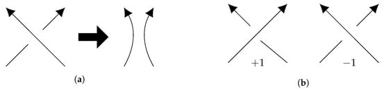
Figure 1. (a) Example of a coherent band surgery use to model DNA recombination; (b) Contribution of each type of crossing to the projected writhe calculation.

One of the primary goals of knot theory is to distinguish between link types. Knot theory is the mathematical study of links, i.e., embeddings of one or more disjoint circles in three-dimensional space. Each circle is a component of the link. A knot is a link with one component. Two links are topologically equivalent if there is an ambient isotopy between them. Intuitively, two links are equivalent if one can be smoothly deformed into the other without allowing phantom crossings between the curves. Each equivalence class is called a link type, and throughout this paper we may refer to an equivalence class as an isotopy class.

Traditionally, links have been tabulated following the Alexander–Briggs notation [1] that organizes them by their minimal crossing number. The order of the links sharing the same crossing number is somewhat arbitrary. The link table in most common use is the Rolfsen table [2]. There, links are labeled using Conway’s notation [3] and an extension of the Alexander–Briggs notation [1]. In the Rolfsen table, each knot diagram represents the unoriented knot K and its mirror image $K^{*}$. For a link of two or more components, in addition to L and $L^{*}$, the link diagram represents the link type with any component relabeling. However, the link L and its mirror image $L^{*}$ may be in different isotopy classes (i.e., may not be topologically equivalent). Such links are known as chiral links. Similarly, one could orient the link or label the components in several different ways which may yield non-equivalent links. Links which differ only in these ways share many properties, and are represented by a single unoriented link diagram in the standard link tables. In sum, the Rolfsen table provides no way to refer to chirality, orientations or component labeling [2]. Hence, there has been a need to provide explicit diagrams in studies requiring any of this information. The objective here is to provide a link table that accounts for chirality, orientation, and component labeling.

One could of course compile yet another table with an arbitrary choice of mirroring, orientation, and component labeling motivated by an application at hand. Far from solving the problem, this would lead to further confusion. We instead propose to use geometric and topological properties of links to determine a standard diagram for each link. Our goal is to achieve a more clear relationship between isotopy classes of different link types. This is particularly useful when studying enzymatic actions and trying to establish relationships of link types before and after crossing changes or coherent band surgery (Figure 2). More specifically, we propose to use writhe and linking number (introduced in Section 2) to classify the different isotopy classes formed by mirroring, orientation reversal, and component relabeling.

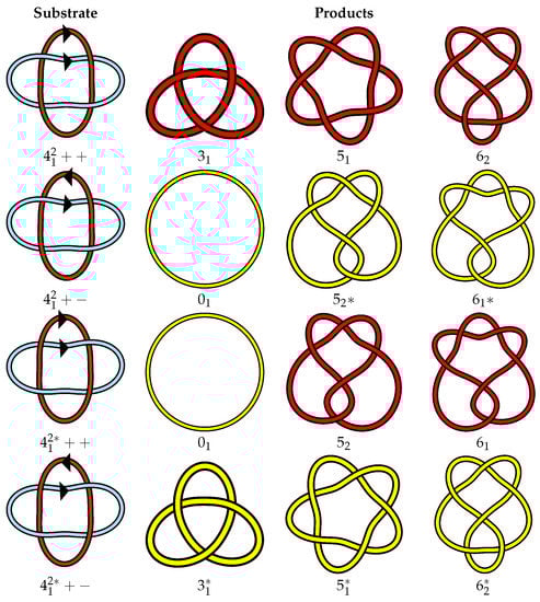
Figure 2. Isotopy types of the link $4_1^2$ are pictured in the first column. Each row denotes a different isotopy type of the $4_1^2$ used as the starting point for a coherent band surgery (local reconnection). These can be interpreted as substrates of site-specific recombination at two dif sites, one on each component of the link. The right side shows all the potential products of said event, up to crossing number 6, depending on the isotopy type of the substrate. It is clear in this example that coherent band surgery on the different isotopy types of the link $4_1^2$ yields different knots. In particular, $4_1^2$+− and $4_1^{2*}$++ can be unknotted in one step, while $4_1^2$++ and $4_1^{2*}$+− cannot.

Here by “classify”, rather than any deeper topological classification, we mean to distinguish isotopy classes of links in such a way that they can be consistently referenced. In Section 3, we review previous efforts in this direction. In Section 4, we propose a classification based on linking number and total writhe (defined in Section 2) and define a canonical isotopy class for links. In Section 4 we define the BFACF algorithm. In Section 5, we use numerical data obtained from BFACF simulations to estimate the total writhe for all prime links with up to nine crossings. In Section 6 we describe the numerical methods. We use self-avoiding polygons in ${\mathbb{Z}}^3$ to represent knots and links with two components. For any given polygon length n, we estimate the mean writhe values of all length n representations of a given isotopy class. This extends previous work on knots [4,5] and our numerical methods may be applied to any other link type.

Portillo et al. conjectured that given a chiral knot K, the mean writhe of all length n conformations in ${\mathbb{Z}}^3$ is bounded as n varies, and furthermore is either positive for all n or negative for all n [4]. The numerical data in [4] for knots with up to eight crossings supported this conjecture. Brasher et al. [5] extended the numerical work to knots with up to 10 crossings; their data remained consistent with the conjecture. Table S6 is the table of canonical knot diagrams extended from that presented by Brasher et al. [5]. We extend the conjecture to links as follows:

Conjecture 1.

Given a c-component link L, the mean of the self-writhe for each component is bounded as the total link length n varies. Moreover, if the link is chiral, then the sum of these mean self-writhes is either positive for every n or negative for every n.

Here, the total link length n is defined as the sum of the component lengths. Additionally, we could conjecture that if a link L with c components has a property that exchanging component i with component j yields a different link (i.e., L lacks exchange symmetry between components i and j), then for any total link length n, either the mean self-writhe of component i is smaller than the mean self-writhe of component j, or vice versa. We find, however, that, for smaller values of n, this ordering may not be consistent. Specifically, minimum length conformations of the $8_{15}^2$ link are provided as a counterexample (see Section 5).

Based on Conjecture 1 and the supporting numerical data presented in Section 5 and in the supplementary materials (online), we propose the following nomenclature. Let $\mathcal{L}$ be the set consisting of an oriented link and all links obtained from it by mirroring, component reversal and relabeling. We choose the standard link diagram L representative of the set $\mathcal{L}$ as the one corresponding to an isotopy class where the sum of self-writhes and linking number are most positive, with components labeled in order of decreasing self-writhe.

We argue that this is a natural approach to choose the standard link diagram since writhe and linking number are very closely related to chirality (see Section 3.4), and since we find that component self-writhe is related to exchange symmetries (i.e., component relabeling). Among the 2-component links with crossing number up to 9, only five are not fully disambiguated by our method. It is worth noting that previous approaches only partially disambiguate link isotopy classes (see Section 3.5 and Section 4.2 for more details). Additionally, the numerical methods used here to explore random conformations have been extensively used in studies of random knotting in the simple cubic lattice ${\mathbb{Z}}^3$ [6,7], and in applications to DNA studies. For example to explore whether or not biological processes, such as those performed by topoisomerases and recombinases, are truly random or have some order [8]. Relevance of proper link identification in DNA topology is discussed at the end of this section.

The structure of the paper is as follows. We start in Section 2 by defining writhe and linking number, which we will use to help distinguish the symmetry classes. Link symmetries and existing nomenclatures are reviewed and extended in Section 3. We describe a systematic way to define a canonical isotopy class for each link (Figure A1) in Section 4. In Section 5, we discuss the results of the numerical simulations used to distinguish between isotopy classes of links, and how they relate to Conjecture 1. Additional numerical results are included in the Supplementary Materials online. In Section 5, we also prove Theorem 2 that determines the difference in writhe between two polygons related by BFACF moves. This theorem deals with the boundedness of writhe for lattice links within the same isotopy class. The numerical methods used are described in Section 6. The key outcome of our work is Figure A1, the table of oriented link diagrams with labeled components based on our proposed nomenclature. For completeness, we have included Table S6, the writhe-based knot table extended to 10 crossings based on the work of Portillo et al. and Brasher et al. [4,5].

Importance of Link Symmetries in DNA Topology

Complete distinction between links related by reflection, orientation changes, and component relabeling is important in many problems in physics and biology. Our motivation for this study comes from the need to unambiguously identify knots and links arising from biological processes that change the topology of DNA. In its most common form, the B form, DNA forms a right-handed double helix consisting of two sugar phosphate backbones held together by hydrogen bonds. The backbones have an inherent antiparallel chemical orientation ($5^{\prime }$ to $3^{\prime }$) and a circular molecule could be modeled as an orientable 2-component link where each backbone is represented by one link component.

More often, in DNA topology studies, the molecule is modeled as the curve drawn by the axis of the double helix. The axis can inherit the orientation of one of the backbones or be assigned an orientation based on its nucleotide sequence. In this way, one circular DNA molecule is modeled naturally as an oriented knot and two interlinked molecules are modeled as oriented 2-component links.

Different cellular processes can alter the topology of DNA. A notable example is that of replication of circular DNA. Replication is the process that makes two identical copies of a chromosome in preparation for cell division. If the chromosome is circular, as in the case of bacteria, replication gives rise to two interlinked chromosomes. If the original DNA circle is unknotted, then the newly replicated link is a right-handed torus link of type $T(2,N)=N_1^2$ (Figure 2) [9]. The orientation given to the DNA circle before replication is naturally inherited by the components of the newly replicated link. Replication links are typically unlinked by enzymes in the family of type II topoisomerases which simplify the topology of their substrate DNA by a sequence of crossing changes. In [10], Grainge et al. showed that in Escherichia coli, in the absense of the topoisomerase Topo IV, replication links could be unlinked by site-specific recombination. Site-specific recombinases act by local reconnection, which can be modeled as a coherent band surgery on the substrate link (see Figure 1a). This process was studied in [8,11]. Importantly, the outcome of recombination can be dependent on the exact symmetry class of the link being acted on as illustrated in Figure 2.

Furthermore, links arising as products of enzymatic reactions on circular substrates may have distinguishable components if the nucleotide sequence differs from one component to the other. In addition, some enzymes in the group of topoisomerases and site-specific recombinases have been found to have a chirality bias when identifying their targets (topological selectivity) or to tie knots or links of particular topology and symmetry type (topological specificity).

2. Writhe and Linking Number

Linking number is a standard topological invariant of oriented links which may be calculated from a spatial conformation or a regular diagram. To calculate linking number of an oriented link L from a regular diagramof L, number the inter-component crossings from 1 to m, and assign characteristic ${ϵ}_i$ to crossing i, where ${ϵ}_i$ is either $+1$ or $-1$ according to the convention in Figure 1b. The linking number is lk$(L)=\frac{1}{2}{\sum }_{i=1}^m{ϵ}_m$. For a 2-component link embedded in space parametrized by curves ${\gamma }_1,{\gamma }_2:{\mathbb{S}}^1\to {\mathbb{S}}^3$, the linking number is calculated by the Gaussian integral

$$\mathrm{lk}(L)=\frac{1}{4\pi }{\int }_{{\gamma }_1}{\int }_{{\gamma }_2}\frac{(d{r}_2\times d{r}_1)·(r_2-r_1)}{|r_2-r_1{|}^3},$$

(1)

where $r_i$ are the vectors representing points along the curve ${\gamma }_i$ [12].

Space writhe is a geometric invariant of a link conformation that measures entanglement complexity. The space writhe of a knot conformation $\sigma$ parametrized by $\gamma :{\mathbb{S}}^1\to {\mathbb{S}}^3$ is found by taking the integral

$$w(\sigma )=\frac{1}{4\pi }{\int }_{\gamma }{\int }_{\gamma }\frac{(d{r}_2\times d{r}_1)·(r_2-r_1)}{|r_2-r_1{|}^3},$$

(2)

where $r_i$ are the vectors representing points along the curve $\gamma$ [12]. Note that space writhe is not a topological invariant.

For links with c components, each component has its own self-writhe calculated as above. We denote self-writhe of component i by $s({\sigma }_i)$ where ${\sigma }_i$ is the conformation of the ith component. The sum of self-writhes of a c-component link conformation $\sigma ={\bigsqcup }_{i=1}^c{\sigma }_i$ is $s(\sigma )={\sum }_{i=1}^{c}s({\sigma }_i)$. We define the total writhe of a link conformation $\sigma$ as $w(\sigma )=s(\sigma )+2lk(\sigma )$. Note that, for a link L with conformation $\sigma$, we can write lk$(\sigma )=$ lk$(L)$ since linking number is an invariant. However, this substitution cannot be made for $s(\sigma )$, as writhe is not a topological invariant.

3. Link Symmetries and Nomenclature

In this section, we define the different types of link symmetries and introduce the proposed link nomenclature.

3.1. Isotopy Classes

Two links are equivalent if there is an ambient isotopy that transforms one into the other. The set of all conformations which are isotopically equivalent form an isotopy class. When a link L is not equivalent to its mirror image L${}^{*}$, then L and L${}^{*}$ form two distinct isotopy classes. However, when link diagrams are listed in a table of unoriented links, only one of these two isotopy classes is represented. It is easy to obtain the mirror image L${}^{*}$ from the diagram of L by changing all over-crossings to under-crossings and vice versa. The number of potential isotopy classes is increased by assigning orientations and labeling components. For an oriented c-component link with labeled components, there are up to $2·2^c·c!$ distinct isotopy classes. This number comes from the 2 reflections, $2^c$ orientations, and $c!$ labelings of the components.

In this paper, we consider links with $c=1$ or 2, but strive to develop methods which can be generalized to $c\in \mathbb{N}$. When $c=1$, there are two possible unoriented isotopy classes (the knot and its mirror image), and four possible oriented isotopy classes. For 2-component links, there are 16 possible isotopy classes for each oriented link with labeled components.

3.2. Doll and Hoste Notation

We use the notation of Doll and Hoste to differentiate isotopy classes of links [13]. Consider an oriented 2-component link of link type L with labeled components. We will refer to this initial link as L++. If we have a link in which the ith component is reversed from L++, then we replace the ith + with a −. If an oriented link is fully invertible (see below), the +’s and −’s may be omitted. The mirror image of L++ is denoted by L${}^{*}+$+. Likewise the mirror images of L+−, L−+, and L−− are L${}^{*}+$−, L${}^{*}-$+, and L${}^{*}-$−, respectively. This notation extends to c-component links by appending another + or − for each additional component. Note that this notation intrinsically assumes the components are labeled numerically from 1 to c.

We propose extending this notation by using an element of the permutation group $S_c$ to denote other possible labelings given L$+\cdots +$. Given $\alpha \in S_c$, we use $\alpha$L$+\cdots +$ to denote L$+\cdots +$ with the ith component relabeled to $\alpha (i)$ for each i. If $\alpha$ is the identity, then it may be omitted. Note that, for 2-component links, $\alpha$ may only be the identity or the permutation exchanging 1 and 2. Applying this notation with reversals leaves an ambiguity for the order in which the relabeling and component reversals happen. For example, if L is a 2-component link and $\tau$ is the transposition of 1 and 2, then which is the reversed component in $\tau$L+−? We take the convention that $\alpha$ is applied to L$\pm \cdots \pm$ after the orientations are determined. This means that the diagrams of L+− and $\tau$L+− will look identical except for the names assigned to the components, which is to say that L+− and $\tau$L+− have the same underlying unlabeled oriented link L+−. Figure 3 illustrates this notation in full for the $4_1^2$ link.

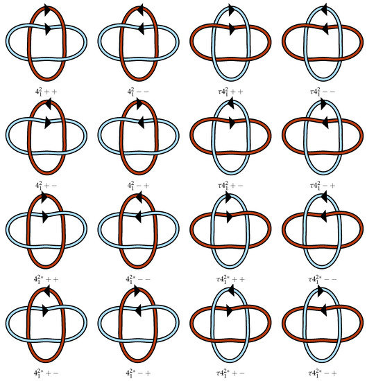
Figure 3. Example of the link notation adopted and modified from the work of Doll and Hoste [13]. The lighter blue strand is component 1 and the darker red-orange strand is component 2. Here, $\tau$ is the nontrivial element of $S_2$. Because $4_1^2$ has symmetry group ${\Sigma }_{4,1}$, all links sharing a row in this figure are equivalent. The diagram labeled $4_1^2$++ here matches the diagram in Figure A1. All other diagrams are determined from $4_1^2$++.

3.3. Link Symmetries

The symmetries of a c-component link can be described by a subgroup of ${\Gamma }_c={\mathbb{Z}}_2\times ({\mathbb{Z}}_2^c⋊S_c)$ [14]. The generator from the first ${\mathbb{Z}}_2$ represents a reflection. The generator of the ith copy of ${\mathbb{Z}}_2$ in ${\mathbb{Z}}_2^c$ represents a reversal of the ith component. A permutation $\alpha \in S_c$ represents a relabeling where component i is relabeled as $\alpha (i)$.

We adopt the notation for symmetry group names used in Cantarella et al. (Figure 1 of [15]). Specifically, each group is given a designation ${\Sigma }_{k,j}$ where k is the order of the group and j is an index (as determined by Cantarella et al. [15]). After cross-referencing with the work of Berglund et al. [14] and Henry and Weeks [16], we found that only 8 of the 27 subgroups occur for 2-component links with crossing number 9 or less. Find details of each of these subgroups in Table 1. The symmetry names used come from the work of Berglund et al. [14] and are defined for a 2-component link L as follows:

Table 1. Symmetry groups for two-component links with up to nine crossings. Listed are names for the groups and their notation as a subgroup of ${\Gamma }_2$ [14,15]. Also listed are generators for the subgroup where $ϵ$ is a reflection, $r_1$ and $r_2$ are reversals of components 1 and 2, respectively, and p is the exchange of the component labels. The final column indicates which of the 16 different possible isotopy classes are equivalent to L++. Here $\tau$ is the non-trivial element of $S_2$.

Symmetry Name	Occurences for $\mathit{c}(\mathit{L})\le 9$	Subgroup of ${\mathbf{\Gamma }}_2$	Generators of Subgroup	Equivalence Class of $\mathit{L}++$
Full Symmetry	1	${\Gamma }_2$	$⟨ϵ,r_1,r_2,p⟩$	$\{L$++, L+−, L−+, L−−, $L^{*}$++,$L^{*}$+−, $L^{*}$−+, $L^{*}$−−, $\tau$L++, $\tau$L+−,$\tau$L−+, $\tau$L−−, $\tau$$L^{*}$++, $\tau$$L^{*}$+−,$\tau$$L^{*}$−+, $\tau$$L^{*}$−−}
Purely Inv. (Pure Ex.)	25	${\Sigma }_{4,1}$	$⟨r_1{r}_2,p⟩$	$\{L$++$,L$−−, $\tau$L++, $\tau$L−−}
Purely Inv. (No Ex.)	32	${\Sigma }_{2,1}$	$⟨r_1{r}_2⟩$	$\{L$++$,L$−−}
Fully Inv. (Pure Ex.)	5	${\Sigma }_{8,1}$	$⟨r_1,r_2,p⟩$	$\{L$++$,L$+−$,L$−+$,L$−−,$\tau$L++, $\tau$L+−, $\tau$L−+, $\tau$L−−}
Fully Inv. (no Ex.)	22	${\Sigma }_{4,2}$	$⟨r_1,r_2⟩$	$\{L$++$,L$+−$,L$−+$,L$−−}
Even Op. (Pure Ex.)	3	${\Sigma }_{8,2}$	$⟨ϵr_1,ϵr_2,p⟩$	$\{L$++, L−−, $L^{*}$+−, $L^{*}$−+, $\tau$L++,$\tau$L−−, $\tau$$L^{*}$+−, $\tau$$L^{*}$−+}
Even Op. (Non-Pure Ex.)	1	${\Sigma }_{4,5}$	$⟨ϵr_{1}p,ϵr_{2}p⟩$	$\{L$++$,L$−−$,\tau L^{*}$+−$,\tau L^{*}$−+}
No Symmetry	3	$\left\{e\right\}$	$⟨e⟩$	$\{L$++}

• L is purely invertible if it is isotopic to the link found by simultaneously reversing both components (L++ = L−−).
• L is fully invertible if it is isotopic to L with every other choice of orientation.
• L has even operations symmetry if it is isotopic to links obtained by an even number of reflections and/or component reversals.
• L has pure exchange symmetry if it is isotopic to L with the component labels exchanged (L++ = $\tau$L++).
• L has a non-pure exchange symmetry if it is isotopic to L with a combination of exchanged labels with a reflection and/or with component reversals, but L++ ≠ $\tau$L++.
• L has no exchange symmetry, if it is not isotopic to L with the component labels exchanged regardless of any reversals or reflections.
• L has full symmetry if it is isotopic to every link obtained by component relabeling, component reversal, and reflection.
• L has no symmetry if it is not isotopic to any link obtained by component relabeling, component reversal, or reflection.

It is interesting to note that of the eight symmetry types observed for prime 2-component links with no more than nine crossings, only links with no symmetry lack any kind of inversion symmetry. More specifically, every prime 2-component link with at most nine crossings has L++ = L−− except for the $9_{34}^2$, $9_{35}^2$, and $9_{39}^2$ links which have no symmetry. In addition, the only links which have any kind of reflection symmetry are those with even operations symmetry or full symmetry. There are only four prime 2-component links with crossing number up to 9 that have even operations symmetry, and the only observed 2-component link with full symmetry is $0_1^2$ [15]. All other prime 2-component links lack reflection symmetry.

For the purposes of classification of isotopy types, the more interesting links are those which lack certain symmetries, as there will be more isotopy classes to disambiguate. As we will see in Section 3.4, writhe is connected to the isotopy class of links which lack pure exchange and/or reflection symmetries. Because of this, those links will be of particular interest to the results of our writhe experiments described in Section 6. Of the 92 prime 2-component links with crossing number 9 or less, 58 lack pure exchange symmetry and 87 lack reflection symmetry.

3.4. Symmetries, Writhe and Linking Number

Consider a 2-component link L++ with linking number lk(L++) $\ne 0$. A link diagram for the mirror image L${}^{*}+$+ can be obtained by taking a diagram for L++ and switching all of the over/under-crossings. This changes the sign of each crossing’s contribution to the linking number, hence lk(L++) $=-$lk(L${}^{*}+$+). Thus, an oriented link with non-zero linking number cannot be equivalent to its mirror image as an oriented link. Note that it could, for example, have even operations symmetry, which would make it equivalent to its mirror as an unoriented link.

Similarly, reversing the orientation of one of the components will change the characteristic of each inter-component crossing, i.e.,

$$\mathrm{lk}(\mathrm{L}++)=\mathrm{lk}(\mathrm{L}--)=-\mathrm{lk}(\mathrm{L}-+)=-\mathrm{lk}(\mathrm{L}+-).$$

(3)

Thus, the linking number can help discern choices of orientation. Note that reversing the orientation of a link component does not change self-writhe of that component.

Taking the mirror image of a link will yield the opposite self-writhes, linking number, and total space writhe. That is, for a c-component link L in conformation $\sigma$ with components ${\sigma }_i$,

$$s({\sigma }_i)=-s({\sigma }_i^{*}),s(\sigma )=-s({\sigma }^{*}),\mathrm{lk}(\sigma )=-\mathrm{lk}({\sigma }^{*}),\mathrm{and}w(\sigma )=-w({\sigma }^{*}),$$

(4)

where ${\sigma }^{*}$ is the reflection of conformation $\sigma$. We observe that writhe is in some way dependent on chirality, but not orientation, whereas linking number is dependent on both.

3.5. Previous Classification Schemes

There have been previous attempts to classify link isotopy classes. For chirality, Liang et al. [17] classified alternating links into chiral designations of either D or L based on a method called writhe profiles, which is related to projected writhes. While writhe profiles provide a useful way to classify many alternating knots and links, they do not classify non-alternating knots and links. Moreover, there is a discrepancy in the work of Liang et al. between how oriented and non-oriented links are classified.

For non-oriented links, in [17] the authors checked the sign of the projected writhe and assigned a D for a positive value and an L for a negative value. If the sum of self-writhes was zero, writhe profiles were calculated in order to specify a designation of D or L. For oriented links, the sign of the linking number was checked first and the link was assigned a D for a positive value and an L for a negative value. If the linking number was zero, the designation process for the non-oriented links was followed with minor changes to account for orientation.

A discrepancy arises when linking number is non-zero. Chirality is a property independent of orientation but linking number very much depends on orientation. Thus, linking number is not a good choice for a chiral designator. To see the issue more clearly, take the link $4_1^2$ as an example. The oriented $4_1^2$ link has four oriented symmetry classes which can be represented by $4_1^2$++, $4_1^2$+−, $4_1^{2*}$++, and $4_1^{2*}$+−(see Figure 3). The unoriented $4_1^2$ link only has two unoriented symmetry classes which could be represented by $4_1^2$ and $4_1^{2*}$. In the classification of Liang et al. [17], the link designated by $4_1^2$++ in Figure 3 would be given a D classification, while $4_1^2$+− would get an L. However, as chirality is a property of the unoriented link and since $4_1^2$++ and $4_1^2$+− both share the same underlying unoriented link representation, $4_1^2$, then in a consistent classification scheme they should be given the same chiral designation.

Our classification method (Section 4) also uses writhe, but only to distinguish and classify link mirrors and component labelings, and we use linking number only to distinguish orientations.

4. Defining a Canonical Isotopy Class for Links

In order to classify link isotopy classes, we use Monte Carlo sampling of self-avoiding polygons of fixed link type in the simple cubic lattice ${\mathbb{Z}}^3$, followed by a writhe calculation. Sampling is done via the BFACF algorithm as described in Section 4.1.

4.1. Cubic Lattice Links and the BFACF Algorithm

The numerical methods of this paper use links in ${\mathbb{Z}}^3$. We refer to these as lattice links. A c-component lattice link is a disjoint union of c self-avoiding polygons. A self-avoiding polygon of length n is a sequence of points $\{v_1,v_2,\dots ,v_n\}$ in ${\mathbb{Z}}^3$ such that $|v_i-v_{i+1}|=1$ for $i=1,2,3,\dots ,n-1$, $|v_n-v_1|=1$, and $v_i\ne v_j$ for all $i\ne j$. To obtain the polygon from these points, we include the edges $e_i$, $i=1,\dots ,n$, where $e_i$ is the edge connecting $v_i$ and $v_{i+1}$, with $e_n$ connecting $v_n$ and $v_1$ (Figure 4b). The length of a link in ${\mathbb{Z}}^3$ is the sum of the lengths of the components of the link. We denote the length of a lattice link $\sigma$ by $\left|\sigma \right|$.

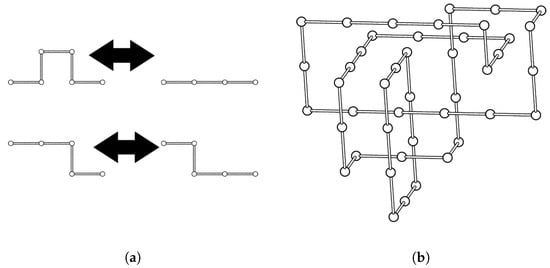
Figure 4. (a) BFACF moves: ($\pm 2$)-move, top; ($+0$)-move, bottom; (b) A minimum step cubic lattice representation of the $8_{15}^2$ link.

This representation is advantageous as it allows us to use the BFACF algorithm to sample a distribution of link conformations and analyze geometric trends such as writhe. The BFACF algorithm is a dynamic Markov chain Monte Carlo algorithm sampling from a state space of self-avoiding polygons in ${\mathbb{Z}}^3$ [18,19,20]. The state spaces are the lattice link isotopy classes. Transitions in the chain are deformations of the link as seen in Figure 4a. Janse van Rensburg and Whittington showed that the ergodicity class of a knot or link in BFACF is the set of all possible embeddings within that knot or link’s isotopy class in ${\mathbb{Z}}^3$ [6].

The transition probabilities of the BFACF algorithm depend on an adjustable parameter $z\in (0,z_0)$ where $z_0\approx 0.2134$ [6]. The limiting distribution of the resulting Markov chain is

$$\pi (\sigma )=\frac{\left|\sigma \right|z^{\left|\sigma \right|}}{\Xi (z)},$$

(5)

where

$$\Xi (z)=\sum _{n=4}^{\infty }n{z}^n{\mu }_n(L),$$

(6)

and ${\mu }_n(L)$ is the total number of length n lattice links in the same isotopy class as L. This distribution has the property that all conformations of the same length have equal probability, dependent only on z and on the link type. Thus, the BFACF algorithm may be used to uniformly sample conformations of certain link isotopy class and length. The reader is directed to ([21], chapter 9) for a full treatment of the BFACF algorithm.

4.2. Canonical Isotopy Class

References to links in the literature most commonly use the name listed in the Rolfsen table [2]. This is effective for communicating general properties of links, but when working with oriented links or links with distinguished components, one must still explicitly draw a picture of the link for full clarity. Doll and Hoste provided a link table which included orientation and component labels in addition to providing a nomenclature for reversing components [13]. While the diagrams in the Doll and Hoste table were chosen in a systematic way (using Conway notation), there is inconsistency in which isotopy classes of each link are actually represented. For example, the two diagrams listed for $7_3^2$ are reflections of each other and are non-isotopic, since $7_3^2$ lacks reflection symmetry.

Our goal is to propose a systematic way to identify a representative isotopy class for each link type. We use writhe and linking number to aid in this. Let ${\mathcal{C}}_n(L)$ be the set of all length n lattice conformations of L. Let the average of the sum of self-writhes of the elements of ${\mathcal{C}}_n(L)$ be ${\mathcal{S}}_n(L)$, i.e.,

$${\mathcal{S}}_n(L)=\frac{1}{|{\mathcal{C}}_n(L)|}\sum _{\sigma \in {\mathcal{C}}_n(L)}s(\sigma ).$$

(7)

Analogously, let ${\sigma }_i$ be the self-avoiding polygon representing the ith component of $\sigma \in {\mathcal{C}}_n(L)$, then we define the average of the self-writhes of component i of L as

$${\mathcal{S}}_n(L,i)=\frac{1}{|{\mathcal{C}}_n(L)|}\sum _{\sigma \in {\mathcal{C}}_n(L)}s({\sigma }_i).$$

(8)

Case 1, L is a knot ($c=1$)

In the case of knots, we follow the writhe-guided nomenclature proposed in Portillo et al. and Brasher et al. [4,5]. This nomenclature specified the canonical knot K as the one where ${\mathcal{S}}_n(K)>0$. In [4,5], the authors also provided numerical data in support of the conjecture that for each chiral knot K, ${\mathcal{S}}_n(K)$ was either consistently positive or consistently negative regardless of n, thus pointing to an unambiguous designation. Using the data from those papers and previously unpublished 10-crossing data, we constructed a table of knots through 10 crossings (Table S6). Note that these knots do not include orientation information, as the methods used do not discern orientations of knots.

Case 2, L is a 2-component link ($c=2$)

The case of 2-component links is more complicated due to the extra link symmetries as detailed in Section 3 and Table 1. We appeal to Conjecture 1 and use self-writhes and linking number to define the canonical isotopy class of a link, and denote it by L++. In particular, we choose L++ so that ${\mathcal{S}}_n$(L++) $>0$, lk(L++) $>0$, and ${\mathcal{S}}_n(L,1)>{\mathcal{S}}_n(L,2)$ when possible. Once L++ is chosen, it can be used as a point of reference for obtaining all other isotopy classes of the link as described in Section 3.2, and illustrated in Figure 3.

As long as ${\mathcal{S}}_n$(L++) $\ne 0$, then half of the isotopy classes will have ${\mathcal{S}}_n$(L++) $>0$. Then, if lk(L++) $\ne 0$, half of those isotopy classes will have lk(L++) $>0$. Then, as long as ${\mathcal{S}}_n(L,1)\ne {\mathcal{S}}_n(L,2)$, half of those isotopy classes will have ${\mathcal{S}}_n(L,1)>{\mathcal{S}}_n(L,2)$. This narrows down the 16 isotopy classes to two potential candidates for L++. If L has pure exchange symmetry, then these candidates are equivalent and the canonical link L++ is chosen to be this isotopy class. There are three 2-component links with crossing number at most nine that lack pure exchange symmetry: $9_{34}^2$, $9_{35}^2$, and $9_{39}^2$. In fact, these links have no symmetry.

The assumptions that ${\mathcal{S}}_n$(L++) $\ne 0$, lk(L++) $\ne 0$, and ${\mathcal{S}}_n(L,1)\ne {\mathcal{S}}_n(L,2)$ depend on the symmetry type of L. If there is reflection symmetry, then it is necessarily true that ${\mathcal{S}}_n$(L++) $=0$ for all n. If ${\mathcal{S}}_n$(L++) $=0$ and there is no reflection symmetry, then we cannot distinguish the link from its mirror image with our methods, but we did not observe this behavior. If there is pure exchange symmetry, then it is necessarily true that ${\mathcal{S}}_n(L,1)={\mathcal{S}}_n(L,2)$. If ${\mathcal{S}}_n(L,1)={\mathcal{S}}_n(L,2)$ and there is no pure exchange symmetry, then we cannot distinguish the different component labelings with our methods, but we did not observe this behavior either. For links with full inversion symmetry, it is necessarily true that lk(L++) $=0$. If lk(L++) $=0$ and L does not have full inversion symmetry, then we cannot distinguish orientations with our methods. This behavior is observed for only two links: $9_5^2$ and $9_{41}^2$.

In Section 6, we describe the numerical methods used to estimate ${\mathcal{S}}_n(L)$, ${\mathcal{S}}_n(L,1)$, and ${\mathcal{S}}_n(L,2)$ for each 2-component link through nine crossings. Section 5 describes results of the numerical simulations, and analytical results on the effect of BFACF moves on the writhe of a lattice polygon. Partial data are presented in Table 2 and Figure 5. Complete data are included in supplementary Tables S2–S5.

Table 2. Columns 2, 3, and 4 show confidence intervals for the average of the sum of self-writhes (${\mathcal{S}}_{200}(L$++)), and self-writhes of components 1 and 2 (${\mathcal{S}}_{200}(L$++$,1)$ and ${\mathcal{S}}_{200}(L$++$,2)$) for length 200 links in ${\mathbb{Z}}^3$. For each 2-component link indicated in column 1, the average is taken over an ensemble of statistically independent length 200 lattice links of type L as described in the numerical methods section. Combined with the linking number (column 7), these confidence intervals are used to determine which diagram appears as L++ in Figure A1. The Rolfsen ([2]) diagram’s designation under our notation is presented in column 5. Column 6 lists which isotopy class is represented by default KnotPlot. Note that the KnotPlot conformations are reflections of those in the Rolfsen table. Symmetry groups (column 8) are taken from the work of Henry and Weeks, Berglund et al., and from SnapPy [14,16,22].

L	${\mathcal{S}}_{200}(\mathit{L})$	${\mathcal{S}}_{200}(\mathit{L},1)$	${\mathcal{S}}_{200}(\mathit{L},2)$	Rolfsen	KP	lk$(\mathit{L})$	Sym
$0_1^2$	[$--$]	[$--$]	[$--$]	$0_1^2$	$0_1^2$++	0	${\Gamma }_2$
$2_1^2$	[$-0.0370.102$]	[$-0.0540.043$]	[$-0.1060.087$]	$2_1^2$	$2_1^2$++	1	${\Sigma }_{8,2}$
$4_1^2$	[$0.7550.877$]	[$0.3910.481$]	[$0.3360.424$]	$4_1^2$${}^{*}$	$4_1^2$+−	2	${\Sigma }_{4,1}$
$5_1^2$	[$1.4011.607$]	[$0.6850.844$]	[$0.6570.822$]	$5_1^2$${}^{*}$	$5_1^2$++	0	${\Sigma }_{8,1}$
$6_1^2$	[$1.6241.692$]	[$0.8120.862$]	[$0.7950.847$]	$6_1^2$${}^{*}$	$6_1^2$++	3	${\Sigma }_{4,1}$
$6_2^2$	[$-0.1560.042$]	[$-0.1440.014$]	[$-0.0670.083$]	$6_2^2$	$6_2^2$++	3	${\Sigma }_{8,2}$
$6_3^2$	[$1.9572.225$]	[$0.9791.207$]	[$0.8921.105$]	$6_3^2$${}^{*}$	$6_3^2$+−	2	${\Sigma }_{4,1}$
$7_1^2$	[$2.1882.364$]	[$1.0271.167$]	[$1.1091.249$]	$7_1^2$${}^{*}$	$7_1^2$++	1	${\Sigma }_{4,1}$
$7_2^2$	[$0.4130.788$]	[$0.2110.509$]	[$0.0930.389$]	$7_2^2$${}^{*}$	$7_2^2$+−	1	${\Sigma }_{4,1}$
$7_3^2$	[$2.6672.728$]	[$1.3181.373$]	[$1.3241.38$]	$7_3^2$${}^{*}$	$7_3^2$++	0	${\Sigma }_{8,1}$
$7_4^2$	[$4.2924.348$]	[$3.9924.04$]	[$0.2890.319$]	$7_4^2$	$7_4^2$${}^{*}+$+	0	${\Sigma }_{4,2}$
$7_5^2$	[$2.5322.602$]	[$2.8432.904$]	[$-0.326-0.286$]	$7_5^2$${}^{*}$	$\tau$$7_5^2$++	2	${\Sigma }_{2,1}$
$7_6^2$	[$1.4111.445$]	[$1.3811.41$]	[$0.0230.042$]	$7_6^2$${}^{*}$	$\tau$$7_6^2$++	0	${\Sigma }_{4,2}$
$7_7^2$	[$3.513.592$]	[$3.4583.527$]	[$0.0360.081$]	$7_7^2$	$7_7^2$${}^{*}+$+	2	${\Sigma }_{2,1}$
$7_8^2$	[$3.2483.324$]	[$3.3043.368$]	[$-0.07-0.03$]	$7_8^2$${}^{*}$	$\tau$$7_8^2$++	0	${\Sigma }_{4,2}$
$8_1^2$	[$2.4432.477$]	[$1.2251.251$]	[$1.2091.235$]	$8_1^2$${}^{*}$	$8_1^2$+−	4	${\Sigma }_{4,1}$
$8_2^2$	[$0.7610.79$]	[$0.3730.396$]	[$0.3790.403$]	$8_2^2$	$8_2^2$${}^{*}+$+	4	${\Sigma }_{4,1}$
$8_3^2$	[$2.8612.907$]	[$1.4351.474$]	[$1.411.449$]	$8_3^2$${}^{*}$	$8_3^2$++	3	${\Sigma }_{4,1}$
$8_4^2$	[$0.8680.94$]	[$0.4170.476$]	[$0.4290.486$]	$8_4^2$${}^{*}$	$8_4^2$+−	4	${\Sigma }_{4,1}$
$8_5^2$	[$1.1711.22$]	[$0.5750.618$]	[$0.5780.62$]	$8_5^2$${}^{*}$	$8_5^2$++	3	${\Sigma }_{4,1}$
$8_6^2$	[$3.293.33$]	[$1.6321.671$]	[$1.6391.678$]	$8_6^2$${}^{*}$	$8_6^2$++	2	${\Sigma }_{4,1}$
$8_7^2$	[$2.8292.864$]	[$1.4151.445$]	[$1.4021.431$]	$8_7^2$${}^{*}$	$8_7^2$+−	1	${\Sigma }_{4,1}$
$8_8^2$	[$-0.0020.033$]	[$0.0060.035$]	[$-0.020.01$]	$8_8^2$	$8_8^2$++	1	${\Sigma }_{8,2}$
$8_9^2$	[$0.7770.92$]	[$0.4710.599$]	[$0.2760.35$]	$8_9^2$	$\tau$$8_9^2$${}^{*}+$+	2	${\Sigma }_{2,1}$
$8_{10}^2$	[$0.8930.927$]	[$0.5940.625$]	[$0.2910.309$]	$8_{10}^2$	$8_{10}^2$${}^{*}+$+	0	${\Sigma }_{4,2}$
$8_{11}^2$	[$4.9444.98$]	[$4.4234.455$]	[$0.5120.534$]	$8_{11}^2$	$8_{11}^2$${}^{*}+$+	2	${\Sigma }_{2,1}$
$8_{12}^2$	[$1.9041.932$]	[$2.4222.447$]	[$-0.526-0.508$]	$8_{12}^2$${}^{*}$	$8_{12}^2$++	0	${\Sigma }_{4,2}$
$8_{13}^2$	[$1.9452.0$]	[$1.9171.965$]	[$0.0180.046$]	$8_{13}^2$${}^{*}$	$8_{13}^2$++	0	${\Sigma }_{4,2}$
$8_{14}^2$	[$3.133.185$]	[$3.173.218$]	[$-0.051-0.022$]	$8_{14}^2$	$8_{14}^2$${}^{*}+$+	2	${\Sigma }_{2,1}$
$8_{15}^2$	[$0.0290.056$]	[$0.0340.048$]	[$-0.010.014$]	$8_{15}^2$	$\tau$$8_{15}^2$${}^{*}+$+	0	${\Sigma }_{4,2}$
$8_{16}^2$	[$0.1880.219$]	[$0.1320.16$]	[$0.050.065$]	$8_{16}^2$	$8_{16}^2$${}^{*}+$+	2	${\Sigma }_{2,1}$

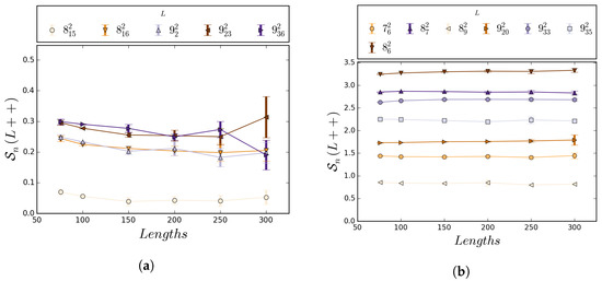
Figure 5. Estimates with 95% confidence intervals for ${\mathcal{S}}_n($L++) for a selection of links for $n\in \{76,100,150,250,\mathrm{and}300\}$. Data were obtained from the simulations as described in Section 6. The expected value of ${\mathcal{S}}_n(8_{15}^2)$ was the lowest among links lacking reflection symmetry. Note that even though the expected value is relatively small for all lengths examined, the confidence intervals do not include 0. Limited variability of ${\mathcal{S}}_n($++) was observed as length increased for all prime links with up to 9 crossings. This suggests a well-behaved nature of writhe for long lattice links. Confidence intervals for all sampled links can be found in Supplementary Table S2. Values shown are for some of the isotopy classes in Figure A1.

4.3. Proposed Link Table

The canonical isotopy class was chosen for each link as described in Section 4.2 using data obtained as described in Section 5 and Section 6. The $9_5^2$, $9_{34}^2$, $9_{35}^2$, $9_{39}^2$, and $9_{41}^2$ links were each narrowed down to two potential candidates by this process, differing by the simultaneous reversal of both components. For each of these links, some extra criterion is required to select a canonical link from the two candidates. We made an arbitrary choice between the two possible candidates for each of these five links, in order to provide a complete table and thus avoid the ambiguities of nomenclature that we set out to eliminate. The canonical or otherwise chosen link diagrams are represented in Figure A1.

4.4. Note on Minimum Lattice Links

In Portillo et al., an ideal lattice knot of type K was defined as a minimal step number (msn) lattice embedding of K [4]. The authors conjectured that the mean writhe of random polygons of given knot type and fixed length could be approximated by the mean writhe of the corresponding ideal msn conformation. They provided numerical evidence that there exists a constant ${\alpha }_K$ such that the mean writhe of a random lattice polygon of type K and length n belongs to $(w_I(K)-{\alpha }_K,w_I(K)+{\alpha }_K)$, independently of the value of n, where $w_I(K)$ is the mean writhe of the ideal lattice conformations of K. We here inquire if this conjecture can be extended to links. Methods and results are presented in Section 5 and Section 6.

5. Results and Discussion

5.1. Numerical Results

Statistically independent ensembles of linked lattice polygons were obtained as described in Section 4.1 and Section 6. We calculated $s(\sigma )$, $s({\sigma }_1)$, and $s({\sigma }_2)$ for each sampled conformation $\sigma$. Using batch mean analysis to account for autocorrelation, these values were used to calculate 95% confidence intervals for ${\mathcal{S}}_n(L)$, ${\mathcal{S}}_n(L,1)$, ${\mathcal{S}}_n(L,2)$ with $n\in \{76,100,150,200,250,300\}$. For each link without reflection symmetry, each confidence interval for ${\mathcal{S}}_n(L)$ was found to be either entirely positive or entirely negative. Moreover, the signs of these confidence intervals are consistent across all sampled lengths for each link as predicted by Conjecture 1.

For links which lack pure exchange symmetry, confidence intervals for ${\mathcal{S}}_n(L,1)$ and ${\mathcal{S}}_n(L,2)$ are disjoint at each n. Moreover, we can choose a labeling of component 1 and component 2 for each link so that ${\mathcal{S}}_n(L,1)>{\mathcal{S}}_n(L,2)$ for $n\in \{76,100,150,200,250,300\}$. From this, we were able to choose canonical link isotopies for most links as described in Section 4. The data for ${\mathcal{S}}_n(L)$, ${\mathcal{S}}_n(L,1)$ and ${\mathcal{S}}_n(L,2)$ for links with up to nine crossings are included in supplementary Tables S2–S4.

A regular diagram for each chosen isotopy class can be found in Figure A1. All data presented in this paper have been converted from sampled isotopy classes to L++ by relabeling components and negating writhe and linking number where appropriate. The confidence intervals of the mean writhes at $n=200$ for links up to crossing number 8 are presented in Table 2 while an extended table including 9-crossing information is included in supplementary materials (Table S5). These tables also list the link isotopy class from Rolfsen’s table and Knotplot using the notation from Section 3.2 based on our choice as L++ [2,15,23].

When the estimated values of ${\mathcal{S}}_n(L)$ and ${\mathcal{S}}_m(L)$ are compared for $n,m\in \{76,100,150,200,250,300\}$, they are found to only vary by a small amount. We estimated $|{\mathcal{S}}_n(L)-{\mathcal{S}}_m(L)|$ for each link, L, and pair of lengths, n and m. The largest difference for ${\mathcal{S}}_n(L)$ was found in the $8_1^2$ link, where ${\mathcal{S}}_{250}(L)$ is estimated to be about $2.411$ compared to $2.589$ for ${\mathcal{S}}_{76}(L)$ for a difference of about $0.178$. Figure 5 illustrates this behavior of ${\mathcal{S}}_n(L)$.

For individual component self-writhe, the largest difference was in ${\mathcal{S}}_n(9_{40}^2,1)$, where ${\mathcal{S}}_{250}(9_{40}^2,1)$ was estimated at $2.439$ compared to $2.211$ for ${\mathcal{S}}_{76}(9_{40}^2,1)$, giving a difference of about $0.228$. For comparison, writhe in ${\mathbb{Z}}^3$ is always a multiple of $1/4$, so no two links or link components can differ in writhe by less than $0.25$ [24]. In this way, ${\mathcal{S}}_n(L)$ and ${\mathcal{S}}_n(L,i)$ appear to be well-behaved.

We also analyzed minimum step links (described in Section 6.2, Table 3 and in the supplementary materials Table S1) and found that ${\mathcal{S}}_{min}(L)$ and ${\mathcal{S}}_{min}(L,i)$ also stayed reasonably close to the other values of ${\mathcal{S}}_n(L)$ and ${\mathcal{S}}_n(L,i)$. We did, however, find ${\mathcal{S}}_{min}(8_{15}^2$++$,1)=0$ and ${\mathcal{S}}_{min}(8_{15}^2$++$,2)\approx 0.2157$, while ${\mathcal{S}}_n(8_{15}^2,1)>{\mathcal{S}}_n(8_{15}^2,2)$ for all other sampled lengths, which shows that component self-writhe of minimum step conformations may not be a sufficient indicator of self-writhe as n increases. We examined the minimum step $8_{15}^2$ conformations in our dataset and observed that component 1 was identical in all of them; it was planar rectangle which always has 0 writhe. One of the minimum step conformations for $8_{15}^2$ can be found in Figure 4b.

Table 3. Mean self-writhes of minimum step prime 2-component links with 8 or fewer crossings. Numbers based on all conformations found in the preprint by Freund et al. [25].

Link	${\mathcal{S}}_{min}(\mathit{L})$	${\mathcal{S}}_{min}(\mathit{L},1)$	${\mathcal{S}}_{min}(\mathit{L},2)$
$0_1^2$	$0.0$	$0.0$	$0.0$
$2_1^2$	$0.0$	$0.0$	$0.0$
$4_1^2$	$0.8125$	$0.4063$	$0.4063$
$5_1^2$	$1.3492$	$0.6746$	$0.6746$
$6_1^2$	$1.65$	$0.825$	$0.825$
$6_2^2$	$0.0$	$0.0$	$0.0$
$6_3^2$	$1.9438$	$0.9719$	$0.9719$
$7_1^2$	$2.1636$	$1.0818$	$1.0818$
$7_2^2$	$0.7$	$0.35$	$0.35$
$7_3^2$	$2.4903$	$2.4427$	$0.0476$
$7_4^2$	$4.2553$	$4.1811$	$0.0743$
$7_5^2$	$2.3625$	$2.7563$	$-0.3937$
$7_6^2$	$1.4375$	$1.4375$	$0.0$
$7_7^2$	$3.5368$	$3.5368$	$0.0$
$7_8^2$	$3.0479$	$3.0479$	$0.0$
$8_1^2$	$2.597$	$1.2985$	$1.2985$
$8_2^2$	$0.8123$	$0.4062$	$0.4062$
$8_3^2$	$2.7172$	$1.3586$	$1.3586$
$8_4^2$	$0.8164$	$0.4082$	$0.4082$
$8_5^2$	$1.1765$	$0.5883$	$0.5883$
$8_6^2$	$3.1666$	$1.5833$	$1.5833$
$8_7^2$	$2.7215$	$1.3607$	$1.3607$
$8_8^2$	$0.0$	$0.0$	$0.0$
$8_9^2$	$0.9355$	$0.6021$	$0.3333$
$8_{10}^2$	$0.9525$	$0.7288$	$0.2236$
$8_{11}^2$	$4.6944$	$4.6667$	$0.0278$
$8_{12}^2$	$2.0538$	$2.2909$	$-0.237$
$8_{13}^2$	$2.1324$	$2.1324$	$0.0$
$8_{14}^2$	$3.0967$	$3.0967$	$0.0$
$8_{15}^2$	$0.2157$	$0.0$	$0.2157$
$8_{16}^2$	$0.5$	$0.5$	$0.0$

5.2. Boundedness of Writhe under BFACF Moves

BFACF moves not only define our sampling method, but also function as Reidemeister moves for lattice links in the sense that any lattice link conformation can be transformed into any other lattice conformation of the same link by a finite sequence of BFACF moves [6]. It is of interest, then, how BFACF moves may affect space writhe. We find that not only do BFACF moves affect space writhe in a bounded way, but writhe changes in a way entirely predicted by the local geometry of the edges within two steps of the BFACF move. To prove this, we will appeal to a special formulation of space writhe for lattice links proven by Lacher and Sumners [26].

To perform the lattice link writhe calculation, we first define the push-off ${\sigma }_{({\epsilon }_1,{\epsilon }_2,{\epsilon }_3)}$ of a lattice link $\sigma$ for ${\epsilon }_i\in (-1,0)\cup (0,1)$. We obtain ${\sigma }_{({\epsilon }_1,{\epsilon }_2,{\epsilon }_3)}$ by translating $\sigma$ along the vector ${\left[{\epsilon }_1,{\epsilon }_2,{\epsilon }_3\right]}^T$.

Theorem 1.

The total writhe of a lattice link may be calculated as follows:

$$w(\sigma )=\frac{lk(\sigma ,{\sigma }_{(\frac{1}{2},\frac{1}{2},\frac{1}{2})})+lk(\sigma ,{\sigma }_{(-\frac{1}{2},\frac{1}{2},\frac{1}{2})})+lk(\sigma ,{\sigma }_{(\frac{1}{2},\frac{1}{2},-\frac{1}{2})})+lk(\sigma ,{\sigma }_{(-\frac{1}{2},\frac{1}{2},-\frac{1}{2})})}{4},$$

(9)

where $lk({\sigma }_i,{\sigma }_j)$ is the linking number of ${\sigma }_i\bigsqcup {\sigma }_j$ [26].

Since we can calculate the total writhe of a link from the self-writhes of the individual components, Equation (9) is sufficient to find writhe for links with any number of components. This yields the following interesting corollary:

Corollary 1.

If σ is a simple cubic lattice representation of a link, then $w(\sigma )=\frac{k}{4}$ for some $k\in \mathbb{Z}$ [26].

A BFACF move is performed by taking an edge of a self-avoiding polygon in ${\mathbb{Z}}^3$ and pushing it one unit in one of the four directions perpendicular to the direction of the edge. We will refer to the edge being pushed as the BFACF edge. If an endpoint of the BFACF edge traces an existing edge of the polygon during that push, then the traced edge is deleted. On the other hand, if an endpoint of the BFACF edge does not trace another edge of the polygon, then an edge is added in the traced space. With this in mind, we prove the following theorem:

Theorem 2.

If ${\sigma }_1$ and ${\sigma }_2$ are related by a single BFACF move, then $|w({\sigma }_2)-w({\sigma }_1)|\le \frac{1}{2}$. More specifically, $\left(w({\sigma }_2)-w({\sigma }_1)\right)\in \{-\frac{1}{2},-\frac{1}{4},0,\frac{1}{4},\frac{1}{2}\}$.

Proof. 

We will consider the BFACF move which transforms ${\sigma }_1$ into ${\sigma }_2$. Without loss of generality, we may assume that

• the BFACF edge runs from $(0,0,0)$ to $(0,1,0$), and
• the result of the BFACF move will push the BFACF edge to an edge from $(0,0,-1)$ to $(0,1,-1)$.

We may rotate and translate the conformation to make these assumptions true, which will not affect the writhe of the conformations.

Now consider the BFACF move. This move may pass the lattice through one of the push-offs from Theorem 1, changing the linking number of the polygon with that push-off. One such strand passage will change the linking number by $\pm 1$, in turn changing the space writhe by $\pm 1/4$. If the move passes the polygon through a push-off edge, then the push-off edge must have endpoints $(-1/2,1/2,-1/2)$ and $(1/2,1/2,-1/2)$ (e.g., the black BFACF edge and orange push-off edge in Figure 6). Checking where this edge must come from in the original polygon by reversing the push-off, we see it is necessary that this edge either has an endpoint at $(0,0,0)$ or at $(0,0,-1)$. In the former case, this means that the edge before to the BFACF edge runs in the x-direction, and there are two such possible edges. In the latter case, the edge before the BFACF edge must run from $(0,0,-1)$ to $(0,0,0)$ and the edge before that must run in the x-direction, and there are two such possible edges. If there is no edge from $(0,0,-1)$ to $(0,0,0)$, then this second case will result in a self-intersection of the link and is not a valid BFACF move. We can see that the four possible edges to result in this change are all mutually exclusive, so from all of these cases, only one can contribute the $\pm 1/4$ change in writhe.

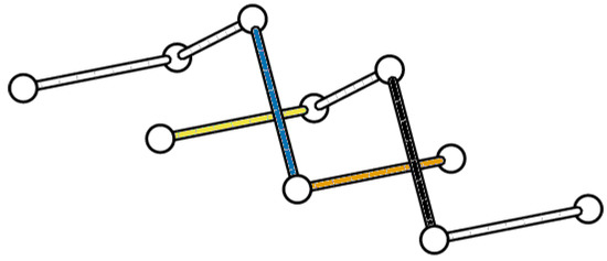
Figure 6. If a BFACF move is performed on the black edge in the direction of the orange (medium gray in grayscale) edge of the push-off beneath it, then the linking number with the push-off will change by $-1$ which will change the writhe by $-1/4$. This same BFACF move will also push the blue (dark gray) edge of the push-off through the yellow (light gray) edge of the link, which will cause the linking number to change by another $-1$, hence this will contribute a $-1/4$ change to the writhe. Thus, a BFACF move pushing the black edge into the page will result in a lattice link with a writhe $1/2$ less than the current link’s writhe.

Now suppose that one of the push-offs of the BFACF edge passes through an edge of the original link when the BFACF move is performed (e.g., the blue push-off edge being pushed through the yellow edge in Figure 6). The four push-offs of the BFACF edge run from $(-1/2,1/2,-1/2)$ to $(-1/2,3/2,-1/2)$, $(1/2,1/2,-1/2)$ to $(1/2,3/2,-1/2)$, $(-1/2,-1/2,-1/2)$ to $(-1/2,1/2,-1/2)$, and $(1/2,-1/2,-1/2)$ to $(1/2,1/2,-1/2)$. We note that in each of these cases the edge which the crossing change is occuring with must be running in the x-direction and have an endpoint at either $(0,1,0)$ or $(0,1,-1)$. Similar to the previous cases, each of these possible edges are mutually exclusive and must either be the edge after the BFACF edge or the edge after that. Again, since they are mutually exclusive cases, the change in writhe from these cases can only be $\pm 1/4$.

Thus, at most two of the above cases may be true at any given time, each contributing to a change in writhe of $\pm 1/4$. Thus, the total change in writhe from any BFACF move is in the set $\{-\frac{1}{2},-\frac{1}{4},0,\frac{1}{4},\frac{1}{2}\}$. ☐

6. Numerical Methods

6.1. BFACF Simulations

We use methods adopted from Portillo et al. and Brasher et al. to procure estimates of ${\mathcal{S}}_n(L)$, ${\mathcal{S}}_n(L,1)$, and ${\mathcal{S}}_n(L,2)$ for 2-component links [4,5]. in particular, BFACF was run to sample conformations of the 91 prime non-split 2-component links with crossing number less than or equal to 9. Only one isotopy class was sampled for each link, as the writhe values for other isotopy classes will be either identical or of opposite sign (as described in Section 3.4). Choices of z values were chosen based on prior systematic runs used to estimate the expected length of the conformations. These same runs were also used to estimate the required number of steps between samples for statistical independence of samples. Statistical independence for these prior runs was determined by calculating integrated auto-correlation.

Samples were taken for links of length 76, 100, 150, 200, 250, and 300. Up to $\mathrm{20,000}$ independent samples were taken for most lengths of each link, with up to $2\times {10}^6$ and $2\times {10}^5$ independent samples for lengths 100 and 150, respectively. Initial sampling was done for lengths 100 and 150, but in many cases runs were terminated before all samples were taken to free up computational resources, as analysis showed the number samples already taken provided sufficiently narrow confidence intervals. For the other lengths, 20,000 was selected as a sufficiently large number for the level of confidence desired. Samples were discarded and not counted if their length did not match the target length for the run.

Once the samples were obtained, the component self-writhes and the sums of self-writhes were calculated. This resulted in three lines of data for each component: the sum of self-writhes; component 1 self-writhe; and component 2 self-writhe. Batch mean analysis was then used to ensure statistical independence of these data and to calculate 95% confidence intervals for the mean of each of these values [27]. Batch mean analysis is a method, which puts sequential data into blocks, if necessary, to reduce auto-correlation and uses the average of each block as a data point.

Before fully analyzing the results, we double-checked the robustness of the sampling methods by comparing certain results to known facts. First, every link with reflection symmetry must have a mean sum of self-writhes which is exactly zero. Hence, the confidence interval for ${\mathcal{S}}_n(L)$ must contain zero for these links. This was true of each link with symmetry group ${\Sigma }_{8,2}$ and ${\Sigma }_{4,5}$ that we sampled, and can be seen in Figure 7a.

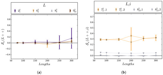
Figure 7. (a) This graph shows 95% confidence intervals for ${\mathcal{S}}_n($L++) of the four links with reflection symmetry and crossing number up to 9, for lengths 76, 100, 150, 200, 250, and 300; (b) This graph illustrates the expected behavior of ${\mathcal{S}}_n(L,i)$ for a link with pure exchange symmetry ($7_2^2$) and a link without pure exchange symmetry ($8_{15}^2$), where i denotes the component number. The large error bars are due to a smaller sample size for $7_2^2$ at length 200; however, even for low sample sizes, the error bars overlap as expected.

In addition, for each link with the pure exchange symmetry, the mean self-writhes of each component must be exactly equal, i.e., ${\mathcal{S}}_n(L,1)={\mathcal{S}}_n(L,2)$. To check for this, we made sure the confidence intervals for ${\mathcal{S}}_n(L,1)$ and ${\mathcal{S}}_n(L,2)$ had non-empty intersection for links with symmetry group ${\Sigma }_{4,1}$, ${\Sigma }_{8,1}$, or ${\Sigma }_{8,2}$ (see Figure 7b). The samples taken for links with these symmetries matched our expectations as well. Thus, the methods appear to have sampled satisfactorily.

We did, however, require extra samples for the $8_{15}^2$ link at lengths 200, 250, and 300. Since $8_{15}^2$ lacks pure exchange symmetry, it is expected that ${\mathcal{S}}_n(L,1)\ne {\mathcal{S}}_n(L,2)$. The data showed this for lengths 76, 100, and 150. However, as length of a link increases, the variance of writhe also increases, which means more samples are required to maintain the same width of confidence intervals as for smaller lengths. For the $8_{15}^2$ link, the self-writhes of the components are both relatively small and close together, which means they must have particularly tight confidence intervals to ensure they are disjoint. For lengths 200, 250, and 300, the confidence intervals for the self-writhe of each component were not disjoint in the original sampling of $8_{15}^2$, which meant uncertainty as to whether they were distinct or if one was larger than the other. Extra samples were taken for these lengths, and with about 45,000 total samples at each length, the intervals were found to be disjoint for lengths 200 and above, matching the data for lower lengths.

The Hopf link, $2_1^2$ provided another issue, in that it is difficult to sample efficiently. Analysis of the autocorrelation of writhe and length of the Hopf link under BFACF moves shows that many more steps may be required between samples. In addition, a high variance of length appears to cause many samples to be rejected. Because of this, the data for $2_1^2$ is somewhat sparse. However, $2_1^2$ has even operations symmetry with pure exchange, which means there are only 2 isotopy classes. Since the linking numbers of these classes are 1 and $-1$, we choose $2_1^2$++ such that lk$(2_1^2$++$) =1$. It is also worth noting that, due to the symmetry of $2_1^2$, it is necessary that ${\mathcal{S}}_n(2_1^2)={\mathcal{S}}_{n,1}(2_1^2)={\mathcal{S}}_{n,2}(2_1^2)=0$. Therefore sampling here serves only to test the robustness of our methods as described above.

The unlink, $0_1^2$, was not sampled, as BFACF fails to converge for split links without extra restrictions such as confinement. The unlink has full symmetry, however, so there is only one choice for isotopy class and every unlink is the canonical unlink. The complete set of confidence intervals for ${\mathcal{S}}_n(L)$, ${\mathcal{S}}_n(L,1)$, and ${\mathcal{S}}_n(L,2)$ for all 2-component links with nine or less crossings can be found in supplementary Tables S2–S4.

6.2. Minimum Length Links

In addition to these BFACF simulations, results were obtained for minimum length lattice links from preliminary data produced by Freund et al. [25]. The data obtained were the set of all known minimum length conformations of each 2-component link with crossing number up to 9. We took the assumption that these sets of conformations were complete, and calculated the mean self-writhes of the minimum lengths directly. We use the notation ${\mathcal{S}}_{min}(L)$, ${\mathcal{S}}_{min}(L,1)$, and ${\mathcal{S}}_{min}(L,2)$ to refer to the mean self-writhes of the minimum length lattice links and their components. We took only the set of conformations representing L++, as determined here, for each link. The results through eight crossings are presented in Table 3, and the results through nine crossings can be found in the supplementary materials in Table S1.

7. Conclusions

Using the BFACF algorithm, we here provide numerical support for Conjecture 1 for each of the ninety-two prime 2-component links with up to 9 crossings. Our results show that, on average, the values of component self-writhes maintain an ordering for sufficiently long lattice links. Using the linking number and the gathered writhe data we are able to unambiguously designate a canonical isotopy class for each prime 2-component link with crossing number up to 9, except for $9_5^2$, $9_{34}^2$, $9_{35}^2$, $9_{39}^2$, and $9_{41}^2$. These five exceptional links are not fully disambiguated by our method; in each case we chose one out of two possible isotopy classes for inclusion in our link table. Figure A1 includes all regular minimal diagrams corresponding to the canonical isotopy classes of 2-component links with 9 or fewer crossings. This table can be used in conjunction with the provided nomenclature to clearly communicate precise link isotopy classes in future research. In addition, we prove a theorem about the boundedness of changes in writhe under the BFACF moves. This result can be useful in proving or finding a counterexample to conjecture 1.

References

- Briggs, G. On types of knotted curves. Ann. Math. 1927, 28, 562–586. [Google Scholar]
- Rolfsen, D. Knots and Links; AMS/Chelsea Publication Series; AMS Chelsea Pub.: Providence, RI, USA, 1976. [Google Scholar]
- Conway, J.H. An enumeration of knots and links, and some of their algebraic properties. In Computational Problems in Abstract Algebra; Elsevier: Amsterdam, The Netherlands, 1970; pp. 329–358. [Google Scholar]
- Portillo, J.; Diao, Y.; Scharein, R.; Arsuaga, J.; Vazquez, M. On the mean and variance of the writhe of random polygons. J. Phys. A Math. Theor. 2011, 44, 275004. [Google Scholar] [CrossRef] [PubMed]
- Brasher, R.; Scharein, R.G.; Vazquez, M. New biologically motivated knot table. Biochem. Soc. Trans. 2013, 41, 606–611. [Google Scholar] [CrossRef] [PubMed]
- Janse Van Rensburg, E.; Whittington, S. The BFACF algorithm and knotted polygons. J. Phys. A Math. Gen. 1991, 24, 5553. [Google Scholar] [CrossRef]
- Janse Van Rensburg, E.J.; Orlandini, E.; Sumners, D.W.; Tesi, M.C.; Whittington, S.G. The Writhe of Knots in the Cubic Lattice. J. Knot Theory Its Ramif. 1997, 6, 31–44. [Google Scholar] [CrossRef]
- Stolz, R.; Yoshida, M.; Brasher, R.; Flanner, M.; Ishihara, K.; Sherratt, D.J.; Shimokawa, K.; Vazquez, M. Pathways of DNA unlinking: A story of stepwise simplification. Sci. Rep. 2017, 7, 12420. [Google Scholar] [CrossRef] [PubMed]
- Adams, D.E.; Shekhtman, E.M.; Zechiedrich, E.L.; Schmid, M.B.; Cozzarelli, N.R. The role of topoisomerase IV in partitioning bacterial replicons and the structure of catenated intermediates in DNA replication. Cell 1992, 71, 277–288. [Google Scholar] [CrossRef]
- Grainge, I.; Bregu, M.; Vazquez, M.; Sivanathan, V.; Ip, S.C.; Sherratt, D.J. Unlinking chromosome catenanes in vivo by site-specific recombination. EMBO J. 2007, 26, 4228–4238. [Google Scholar] [CrossRef] [PubMed]
- Shimokawa, K.; Ishihara, K.; Grainge, I.; Sherratt, D.J.; Vazquez, M. FtsK-dependent XerCD-dif recombination unlinks replication catenanes in a stepwise manner. Proc. Natl. Acad. Sci. USA 2013, 110, 20906–20911. [Google Scholar] [CrossRef] [PubMed]
- Klenin, K.; Langowski, J. Computation of writhe in modeling of supercoiled DNA. Biopolymers 2000, 54, 307–317. [Google Scholar] [CrossRef]
- Doll, H.; Hoste, J. A tabulation of oriented links. Math. Comp. 1991, 57, 747–761. [Google Scholar] [CrossRef]
- Berglund, M.; Cantarella, J.; Casey, M.P.; Dannenberg, E.; George, W.; Johnson, A.; Kelley, A.; LaPointe, A.; Mastin, M.; Parsley, J.; et al. Intrinsic Symmetry Groups of Links with 8 and Fewer Crossings. Symmetry 2012, 4, 143–207. [Google Scholar] [CrossRef]
- Cantarella, J.; Cornish, J.; Mastin, M.; Parsley, J. The 27 Possible Intrinsic Symmetry Groups of Two-Component Links. Symmetry 2012, 4, 129–142. [Google Scholar] [CrossRef]
- Henry, S.R.; Weeks, J.R. Symmetry Groups of Hyperbolic Knots and Links. J. Knot Theory Its Ramif. 1992, 1, 185–201. [Google Scholar] [CrossRef]
- Liang, C.; Cerf, C.; Mislow, K. Specification of chirality for links and knots. J. Math. Chem. 1996, 19, 241–263. [Google Scholar] [CrossRef]
- Berg, B.; Foerster, D. Random paths and random surfaces on a digital computer. Phys. Lett. B 1981, 106, 323–326. [Google Scholar] [CrossRef]
- De Carvalho, C.A.; Caracciolo, S. A new Monte-Carlo approach to the critical properties of self-avoiding random walks. J. Phys. 1983, 44, 323–331. [Google Scholar] [CrossRef]
- De Carvalho, C.A.; Caracciolo, S.; Fröhlich, J. Polymers and g| φ| 4 theory in four dimensions. Nucl. Phys. B 1983, 215, 209–248. [Google Scholar] [CrossRef]
- Madras, N.; Slade, G. The Self-Avoiding Walk; Probability and Its Applications; Birkhäuser: Basel, Switzerland, 1993. [Google Scholar]
- Culler, M.; Dunfield, N.M.; Goerner, M.; Weeks, J.R. SnapPy, a Computer Program for Studying the Geometry and Topology of 3-Manifolds. Available online: http://snappy.computop.org (accessed on 3 March 2017).
- Hypnagogic Software. KnotPlot. Available online: http://www.knotplot.com/ (accessed on 24 October 2014).
- Laing, C.; Sumners, D.W. Computing the writhe on lattices. J. Phys. A 2006, 39, 3535–3543. [Google Scholar] [CrossRef]
- Freund, G.; Witte, S.; Vazquez, M. Bounds for the Minimum Step Number for 2-Component Links in the Simple Cubic Lattice. 2018. in progress. [Google Scholar]
- Lacher, R.; Sumners, D. Data Structures and Algorithms for Computation of Topological Invariants of Entanglements: Link, Twist and Writhe; Prentice-Hall: New York, NY, USA, 1991. [Google Scholar]
- Fishman, G. Monte Carlo: Concepts, Algorithms, and Applications; Springer Series in Operations Research and Financial Engineering; Springer: New York, NY, USA, 2013. [Google Scholar]
© 2018 by the authors. Licensee MDPI, Basel, Switzerland. This article is an open access article distributed under the terms and conditions of the Creative Commons Attribution (CC BY) license (http://creativecommons.org/licenses/by/4.0/).