Control Chart for Failure-Censored Reliability Tests under Uncertainty Environment


1
Department of Statistics, Faculty of Science, King Abdulaziz University, Jeddah 21551, Saudi Arabia
2
Department of Statistics, UVAS, Lahore, Jhang Campus, Lahore 54000, Pakistani
*
Author to whom correspondence should be addressed.
Symmetry 2018, 10(12), 690; https://doi.org/10.3390/sym10120690
Submission received: 11 November 2018
/
Revised: 18 November 2018
/
Accepted: 21 November 2018
/
Published: 2 December 2018
Abstract
:Existing control charts based on failure-censored (Type-II) reliability tests were designed using classical statistics. Classical statistics was applied for the monitoring of the process when observations in the sample or the population were determined. Neutrosophic statistics (NS) are applied when there is uncertainty in the sample or population. In this paper, a control chart for failure-censored (Type-II) reliability tests was designed using NS. The design of a control chart for the Weibull distribution, which is applied when there is a lack of symmetry using neutrosophic statistics, is given. The proposed control chart was used to monitor the neutrosophic mean and neutrosophic variance, which are related to the neutrosophic scale parameter. The advantages of the proposed control chart over the existing control chart are discussed.
1. Introduction
During the manufacturing process, the monitoring of two variations, which can shift the process from the specified target, is an important task. The presence of only the common cause of variation does not affect the manufacturing process. Yet, the presence of a special cause of variation may cause more defects. The control chart is an effective tool, which is widely used in the industry for monitoring the production process. The control chart gives an immediate indication of when the process is shifted from the set target in the presence of a special case of variation. A timely indication is helpful for engineers to sort out the problems in the production process. Therefore, the main objectives of the control chart are to give a quick indication of the shift in the process, to reduce the number of defective products, and to maintain the high quality of the product. Control charts are designed under the assumption that the production data follow the normal distribution or come from the normal manufacturing process. However, experience show that, in the chemical industry, the processes of cutting tool wear and concentrate production follow a skewed distribution [1]. Therefore, several researchers designed control charts in the case of non-normal underlying distributions. Reference [2] designed a control chart for sign statistics. Reference [3] designed Shewhart control charts in the case of skewed data. Reference [4] presented a chart for a gamma distribution. Reference [5] developed a cost model chart for non-normal data. Reference [6] proposed a median control chart. Reference [7] proposed a chart for the Burr distribution. For more details on such control charts, the reader may refer to [8,9,10,11,12,13,14,15,16,17,18].
In the modern era, every reputable industry and company is trying to enhance the quality of their product. The target of creating high-quality products is achieved only by increasing the average lifetime of the product. The reliability, which is the probability that an equipment or a product performs well for the specified period, is used to measure the high quality of the product. For the monitoring of highly reliable products, it is not possible to wait for a specified number of failures. To save cost and time, time-truncated experiments are important. In Type-I censoring, the time of the experiment is fixed and, in Type-II censoring, the number of failures is fixed. The applications of Type-I censoring, Type-II censoring, and progressive and mixed censoring are found in [19,20,21,22,23,24,25,26].
The Weibull distribution is very popular in the area of quality control and reliability due to its flexibility of parameters. The Weibull distribution, due to its bathtub curve, is fitted well to the reliability phenomena. References [27,28,29] discussed the applications of the Weibull distribution. Reference [30] designed a control chart in which the process follows a Weibull distribution. Reference [31] designed a bootstrap control chart for this distribution. References [32,33] introduced control charts using time-truncated life tests. Recently, Khan et al. [34] designed a control chart for a failure-censored reliability test for the Weibull distribution. A detailed discussion of Type-II censoring control charts can be found in references [19,20,21,22,23,24,25,26].
The existing control chart using Type-II censoring is designed under the assumption that all observations are determined. According to reference [35], “observations include human judgments, and evaluations and decisions; a continuous random variable of a production process should include the variability caused by human subjectivity or measurement devices, or environmental conditions. These variability causes create vagueness in the measurement system.” In this case, a control chart using the fuzzy approach was used for monitoring the process. Therefore, fuzzy logic is applied to the design of control charts when the experiment is not sure about some parameters. Several authors contributed in this area and designed control charts using the fuzzy approach such as reference [36] who introduced fuzzy logic in statistical quality control (SQC). Reference [37] introduced an algorithm using fuzzy approach. Reference [38] discussed the application of fuzzy control charts. Reference [35] proposed a Shewhart control chart using this approach. Reference [39] presented a literature review on fuzzy control charts. Reference [40] worked on a fuzzy U control chart. Reference [41] designed fuzzy variable control charts and Reference [42] also worked on a fuzzy control chart. More details on fuzzy control charts can be found in references [43,44,45,46,47,48,49]. Industrial applications can be found in references [50,51,52,53].
Reference [54] mentioned that traditional fuzzy logic is a special case of neutrosophic logic (NS). According to reference [54], neutrosophic logic can be applied when there exists indeterminacy in the observations or the parameters. Based on neutrosophic logic, reference [55] introduced descriptive neutrosophic statistics (NS). Reference [55] argued that NS is an extension of classical statistics. NS has many applications in a variety of areas. References [56,57] applied NS to study rock roughness issues. References [58,59] designed sampling plans using NS. Recently, reference [60] introduced NS in the area of control charts. They designed an attribute control chart using the neutrosophic statistical interval method (NSIM). Reference [60] designed a variance control chart using the NSIM. They showed the efficiency of charts using NS over those based on classical statistics. Upon exploring the literature, we found no work on the design of control charts for failure-censored reliability tests in the uncertainty environment. In this paper, we focus on the design of such control charts using the NSIM. We hypothesized that the proposed chart using the NSIM would be more adequate and effective in the uncertainty environment than the existing control chart based on classical statistics. The state of the art product is described in the next section. The advantages of the proposed chart and a case study are given in Section 3 and Section 4, respectively. Some conclusions are given in the final section. More details failure censored reliability can be seen in reference [61].
2. State of the Art
The failure time of the complements is measured through complex systems or devices. Therefore, it may be possible that some failure times are undetermined or unclear in terms of measurements. As mentioned earlier, NS is the generalization of the classical statistics that is applied when the observations in the sample are indeterminate or unclear. Suppose that the failure time indeterminacy interval 1, 2, 3, …, , where denotes the determinate part and denotes the indeterminate part, follows the neutrosophic Weibull distribution. Reference [59] introduced the following neutrosophic cumulative distribution function (ncdf) of the Weibull distribution.
where is the neutrosophic shape parameter and is the neutrosophic scale parameter. The neutrosophic Weibull distribution reduces to a neutrosophic exponential distribution when . The average lifetime of the neutrosophic Weibull distribution is shown below.
where is the neutrosophic gamma function.
We designed a failure-censored control chart in the case of the failure time following the neutrosophic Weibull distribution to monitor the neutrosophic average and neutrosophic variance, which are related to . The proposed control chart is stated in the following steps.
- Choose a random sample of the size and begin the test. Continue with the test until are reached and note the ith failure time, say (i = 1, …, ).
- Compute the following statistic under NSIM:where is the specified neutrosophic mean time.
- Declare the process in the control state if where and denote the neutrosophic lower control limit (NLCL) and neutrosophic upper control limit (NUCL), respectively.
The operational process of the proposed control chart consists of two neutrosophic control limits. The proposed control chart under the NSIM is an extension of Khan et al. [34] control chart under the classical statistics. The proposed chart reduces to Khan et al. [34] chart when no uncertain observations or parameters are in the sample or in the population.
Suppose that the process is an in-control state at a neutrosophic scale parameter . The neutrosophic average life is shown in the equation below.
Note here that the proposed chart under NISM is independent of . Reference [60] mentioned that statistic is modeled by the neutrosophic gamma distribution with and (see [60]). The neutrosophic parameter is defined by the equation below.
Note here that 2 with 2 degrees of freedom is modeled by a neutrosophic chi-squared distribution. The probability that the process is an in-control state, say at under the NISM, is derived by using the equation below.
where with 2 represents the neutrosophic distribution function of neutrosophic chi-squared distribution. Similarly, the probability that the process is out-of-control when actually in control at is given by the equation below.
or
The average run length under the NISM is known as the neutrosophic average run length (NARL), which is introduced by Aslam et al. [60] and given by the equation below.
Several special causes of variations may shift the process away from the given target. Let denotes the shifted neutrosophic scale parameter where denotes the shift constant. The neutrosophic average life and parameter at is given by Equations (10) and (11).
Note that is modeled by the neutrosophic gamma distribution having and . The probability of in-control under the NISM at is given by the formula below.
The probability of out-of-control under the NISM at is given by Equation (13) or Equation (14) below.
The NARL for the shifted process is given by Equation (15).
Suppose that denotes the specified value of . The values of are shown in Table 1, Table 2, Table 3 and Table 4 for various values of , and . From Table 1, Table 2, Table 3 and Table 4, we note that, for the same values of other specified parameters, the values of NARL decrease as the neutrophil parameter increases.
The following algorithm under the NISM is applied to determine the neutrosophic control limits and :
- Specify , and .
- Specify and determine the neutrosophic control limits such that .
- Several combinations exist that satisfy the condition . However, choose the combination of the neutrosophic parameters where is very close to .
- Use neutrosophic control limits to find .
3. Advantages of the Proposed Chart
In the NS, by following reference [54], we defined the NARL as where is the average run length (ARL) for the determined part under the classical statistics, is an indeterminate part for , and presents the indeterminacy. When there are certain observations in the sample or in the population, the indeterminate part and under the NS becomes the same as the ARL under the classical statistics. According to reference [57], under the uncertainty settings, a method that provides the indeterminacy interval of NARL is said to be a more efficient and effective method than the method that provides a determined value of ARL1. The values of from the proposed control chart under NISM and ARL1 from Aslam et al. [34] under the classical statistics are in Table 5 at the same levels of all specified control chart parameters. From Table 5, we note that the proposed control chart has the values of in the indeterminacy interval while the existing control chart under the classical statistics provides only the determined values of ARL1. For example, when = 0.1, we have . Thus, the determinate par is ARL1 = 1.45 and the indeterminate part is . Therefore, the indeterminacy interval of is . From this example, it is clear that the proposed control chart has determinate and indeterminate information under the indeterminate situation. Therefore, the proposed control chart is more effective under the indeterminate situation than Aslam et al. [34] chart, which is a special case of the proposed chart.
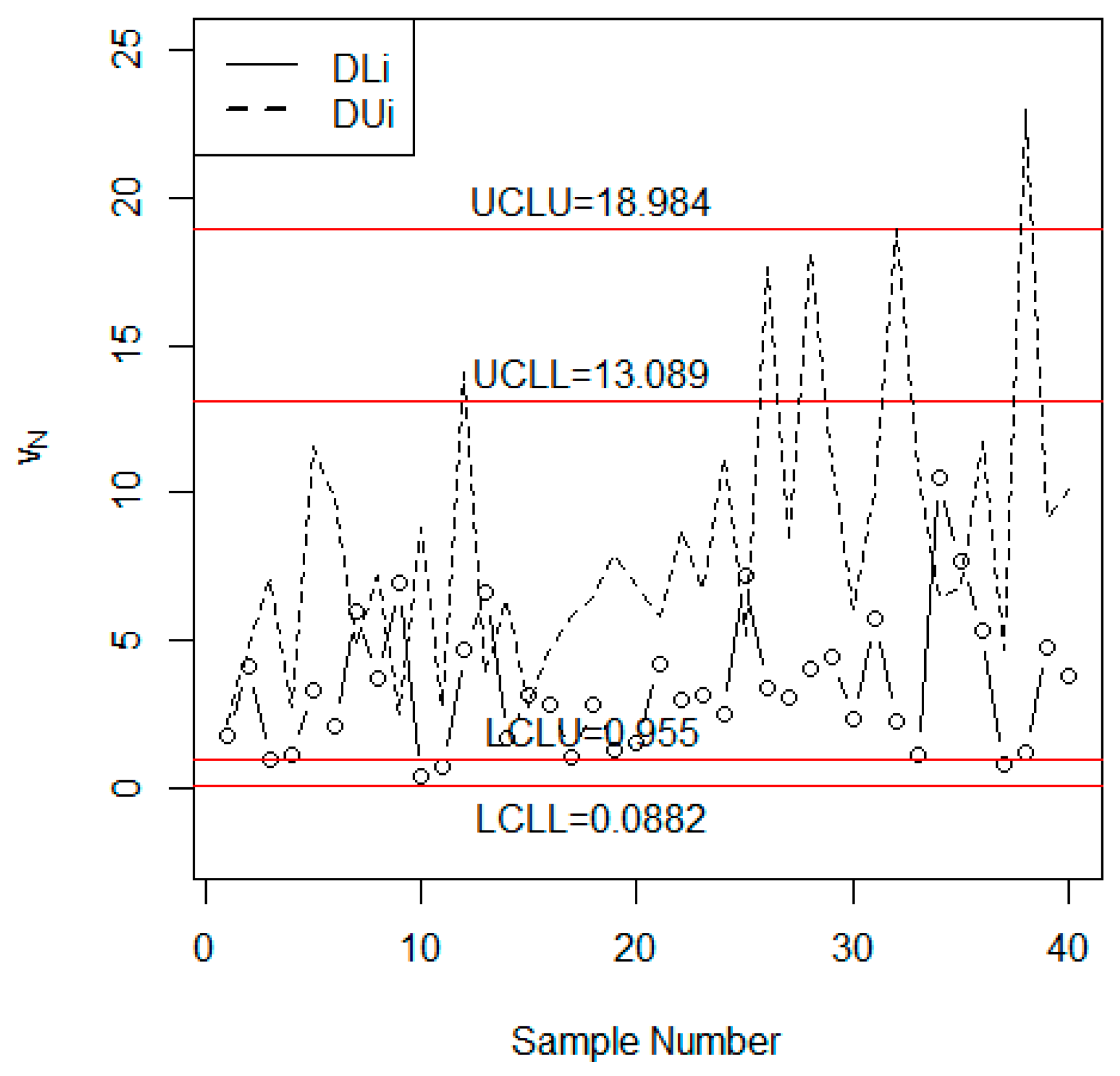
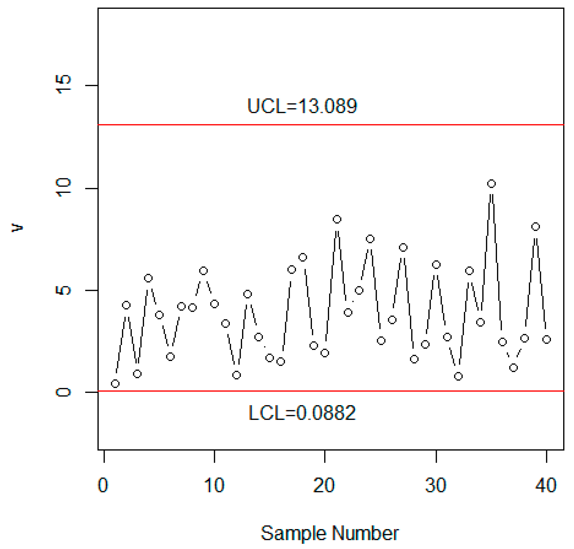
Now, we compare the performance of the proposed control chart under NISM with the chart under the classical statistics using the simulated data. The neutrosophic data was generated from the neutrosophic Weibull distribution with parameters and . The first 20 neutrosophic observations were generated when the process was in-control at and the next 20 neutrosophic observations were generated from the shifted process when = 0.85. From Table 3, the indeterminacy interval of is . Under the uncertainty environment, it is expected that the process will be out-of-control between the 19th and 90th samples when = 0.85. The values of are plotted on the control chart in Figure 1. From Figure 1, we note the proposed control chart under NISM detected a shift at the 39th sample. The values of are also plotted on the existing chart in Figure 2. From Figure 2, we note that the existing control chart under classical statistics did not detect any shift in the process. By comparing Figure 1 with Figure 2, we conclude that the proposed control chart is more efficient in detecting an early shift in the process than the existing chart under classical statistics.
4. Case Study
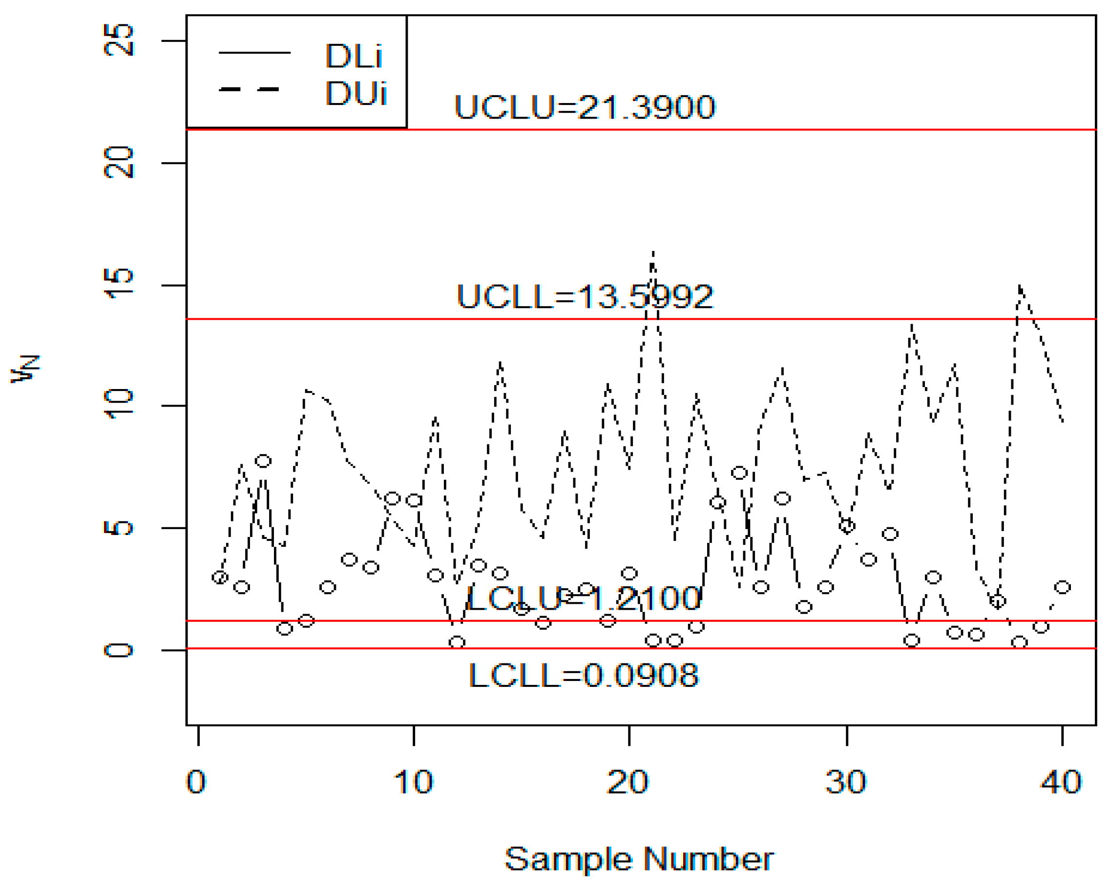
This section is presented to explain the application of the proposed control chart in the very popular automobile manufacturing industry located in Japan. For the high quality of the subsystems of the passenger’s cars, the monitoring of the process is done through the control chart. The quality of the subsystems of the cars is based on the service time. The data is in days until the service is required for the subsystems. The service time data of subsystems is measured through the complex equipment. Therefore, some observations about the time until the service is required are uncertain. The monitoring of such data cannot be done using the control chart proposed by Aslam et al. [34] under classical statistics. Under the uncertainty environment, the company has decided to apply the proposed control chart for the monitoring of service time data. Suppose, for this experiment, the company decided to set parameters as and . The service time data of presenter cars follows the neutrosophic Weibull distribution with and . The for this data is shown in Table 6.
For example, for sample #1: the service time in days is . The statistic for this sample is computed by using the formula below.
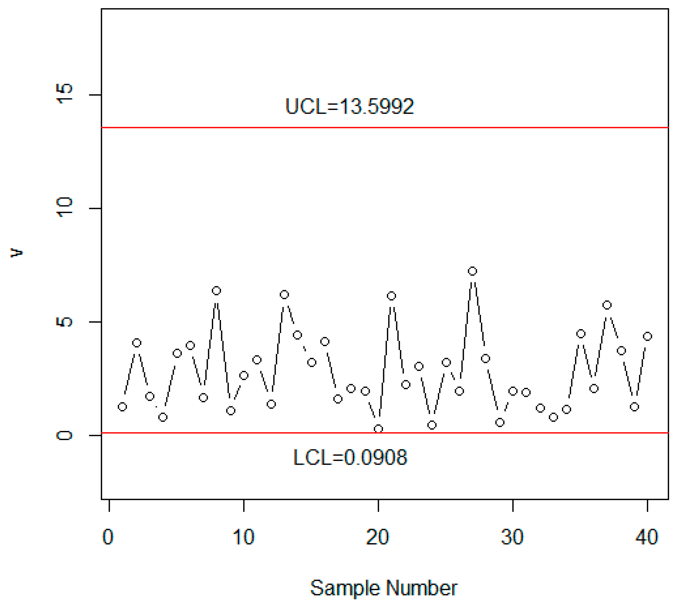
= ; , and . The values of are plotted on the control chart in Figure 3. From Figure 3, we note that several values of the statistic lie in the indeterminacy interval of the control limits. Yet, the control chart proposed by Aslam et al. [34] in Figure 4 shows that the process is an in-control state. From Figure 3, it can be noted that several values of plotting statistics are in the indeterminacy interval. Samples #12, #21, #22, #33, and #37 are very close to the LCLL that needs special attention by the industrial engineers. However, the existing control chart indicates that only two values are very close to the control limit. By comparing Figure 3 with Figure 4, we conclude that the proposed control chart is better, more flexible, and more effective than the existing chart under the uncertainty environment. In addition, the proposed control chart is more efficient for the monitoring of the process than the existing control chart.
5. Conclusions
A control chart for failure-censored (Type-II) reliability tests under the NS was presented in this paper. The necessary measures to apply the proposed control chart were given in the paper. The proposed control chart was the generalization of the control chart under classical statistics. A simulation study and real data showed the efficiency of the proposed control chart under the uncertainty environment. By comparing the proposed chart with the chart under the classical statistics, we noted that the proposed chart was more effective, more flexible, and adequate for use in the uncertainty environment. The proposed control chart can be applied in this industry when there are some uncertain, unclear, and fuzzy observations in the sample or in the population. The proposed control chart, when using the other sampling schemes or the cost model, can be studied in future research.
Author Contributions
Conceived and designed the experiments, M.A. (Mohammed Albassam), N.K., and M.A. (Mohammed Albassam) Performed the experiments, M.A. (Mohammed Albassam) and N.K. Analyzed the data, M.A. (Mohammed Albassam) and N.K. Contributed reagents/materials/analysis tools, M.A. (Muhammad Aslam) Wrote the paper, M.A. (Muhammad Aslam)
Funding
This article was funded by the Deanship of Scientific Research (DSR) at King Abdulaziz University, Jeddah. The authors, therefore, acknowledge and thank DSR technical and financial support.
Acknowledgments
The authors are deeply thankful to the editor and reviewers for their valuable suggestions to improve the quality of this manuscript.
Conflicts of Interest
The authors declare no conflict of interest regarding this paper.
References
- Aichouni, M.; Al-Ghonamy, A.; Bachioua, L. Control charts for non-normal data: Illustrative example from the construction industry business. Available online: https://www.google.com.tw/url?sa=t&rct=j&q=&esrc=s&source=web&cd=1&cad=rja&uact=8&ved=2ahUKEwjgz4mTn_zeAhWOFogKHXjbCXIQFjAAegQICRAC&url=http%3A%2F%2Fwww.wseas.us%2Fe-library%2Fconferences%2F2014%2FMalaysia%2FMACMESE%2FMACMESE-10.pdf&usg=AOvVaw1PPU0bV-aBbm7pVZ9wunqY (accessed on 11 November 2018).
- Amin, R.W.; Reynolds, M.R., Jr.; Saad, B. Nonparametric quality control charts based on the sign statistic. Commun. Stat. Theory Methods 1995, 24, 1597–1623. [Google Scholar] [CrossRef]
- Bai, D.; Choi, I. (x) over-bar-control and r-control charts for skewed populations. J. Qual. Technol. 1995, 27, 120–131. [Google Scholar] [CrossRef]
- Al-Oraini, H.A.; Rahim, M. Economic statistical design of control charts for systems with gamma (λ, 2) in-control times. Comput. Ind. Eng. 2002, 43, 645–654. [Google Scholar] [CrossRef]
- Chen, Y.-K. Economic design of x control charts for non-normal data using variable sampling policy. Int. J. Prod. Econ. 2004, 92, 61–74. [Google Scholar] [CrossRef]
- Ahmad, S.; Riaz, M.; Abbasi, S.A.; Lin, Z. On efficient median control charting. J. Chin. Inst. Eng. 2014, 37, 358–375. [Google Scholar] [CrossRef]
- Lio, Y.; Tsai, T.-R.; Aslam, M.; Jiang, N. Control charts for monitoring burr type-x percentiles. Commun. Stat. Simul. Comput. 2014, 43, 761–776. [Google Scholar] [CrossRef]
- Miller, T.; Balch, B. Statistical process control in food processing. ISA Trans. 1991, 30, 35–37. [Google Scholar] [CrossRef]
- Kegel, T. Statistical control of a pressure instrument calibration process. ISA Trans. 1996, 35, 69–77. [Google Scholar] [CrossRef]
- Chou, C.-Y.; Chen, C.-H.; Liu, H.-R. Economic-statistical design of x¥ charts for non-normal data by considering quality loss. J. Appl. Stat. 2000, 27, 939–951. [Google Scholar] [CrossRef]
- Wu, Z.; Xie, M.; Tian, Y. Optimization design of thex & s charts for monitoring process capability. J. Manuf. Syst. 2002, 21, 83–92. [Google Scholar]
- Venkatesan, G. Process control of product quality. ISA Trans. 2003, 42, 631–641. [Google Scholar] [CrossRef]
- Lin, Y.-C.; Chou, C.-Y. On the design of variable sample size and sampling intervals charts under non-normality. Int. J. Prod. Econ. 2005, 96, 249–261. [Google Scholar] [CrossRef]
- Zhang, H.Y.; Shamsuzzaman, M.; Xie, M.; Goh, T.N. Design and application of exponential chart for monitoring time-between-events data under random process shift. Int. J. Adv. Manuf. Technol. 2011, 57, 849–857. [Google Scholar] [CrossRef]
- McCracken, A.; Chakraborti, S. Control charts for joint monitoring of mean and variance: An overview. Qual. Technol. Quant. Manag. 2013, 10, 17–35. [Google Scholar] [CrossRef]
- Addeh, J.; Ebrahimzadeh, A.; Azarbad, M.; Ranaee, V. Statistical process control using optimized neural networks: A case study. ISA Trans. 2014, 53, 1489–1499. [Google Scholar] [CrossRef] [PubMed]
- Celano, G.; Castagliola, P.; Fichera, S.; Nenes, G. Performance of t control charts in short runs with unknown shift sizes. Comput. Ind. Eng. 2013, 64, 56–68. [Google Scholar] [CrossRef]
- Aslam, M.; Azam, M.; Khan, N. X-bar control charts for non-normal correlated data under repetitive sampling. J. Test. Eval. 2015, 44, 1756–1767. [Google Scholar] [CrossRef]
- Pascual, F.; Li, S. Monitoring the weibull shape parameter by control charts for the sample range of type ii censored data. Qual. Reliab. Eng. Int. 2012, 28, 233–246. [Google Scholar] [CrossRef]
- Guo, B.; Wang, B.X. Control charts for monitoring the weibull shape parameter based on type-ii censored sample. Qual. Reliab. Eng. Int. 2014, 30, 13–24. [Google Scholar] [CrossRef]
- Haghighi, F.; Pascual, F.; Castagliola, P. Conditional control charts for weibull quantiles under type ii censoring. Qual. Reliab. Eng. Int. 2015, 31, 1649–1664. [Google Scholar] [CrossRef]
- Chan, Y.; Han, B.; Pascual, F. Monitoring the weibull shape parameter with type ii censored data. Qual. Reliab. Eng. Int. 2015, 31, 741–760. [Google Scholar] [CrossRef]
- Wang, F.K.; Bizuneh, B.; Cheng, X.B. New control charts for monitoring the weibull percentiles under complete data and type-ii censoring. Qual. Reliab. Eng. Int. 2018, 34, 403–416. [Google Scholar] [CrossRef]
- Asadzadeh, S.; Kiadaliry, F. Monitoring type-2 censored reliability data in multistage processes. Qual. Reliab. Eng. Int. 2017, 33, 2551–2561. [Google Scholar] [CrossRef]
- Aslam, M.; Arif, O.H.; Jun, C.-H. An attribute control chart for a weibull distribution under accelerated hybrid censoring. PLoS ONE 2017, 12, e0173406. [Google Scholar] [CrossRef] [PubMed]
- Guo, B.; Wang, B.X.; Xie, M. Arl-unbiased control charts for the monitoring of exponentially distributed characteristics based on type-ii censored samples. J. Stat. Comput. Simul. 2014, 84, 2734–2747. [Google Scholar] [CrossRef]
- Montgomery, D.C.; Runger, G.C. Applied Statistics and Probability for Engineers; John Wiley & Sons: New York, NY, USA, 2010. [Google Scholar]
- Rausand, M.; Høyland, A. System Reliability Theory: Models, Statistical Methods, and Applications; John Wiley & Sons: New York, NY, USA, 2004; Volume 396. [Google Scholar]
- Borror, C.M.; Keats, J.B.; Montgomery, D.C. Robustness of the time between events cusum. Int. J. Prod. Res. 2003, 41, 3435–3444. [Google Scholar] [CrossRef]
- Nelson, P.R. Control charts for weibull processes with standards given. IEEE Trans. Reliab. 1979, 28, 283–288. [Google Scholar] [CrossRef]
- Nichols, M.D.; Padgett, W. A bootstrap control chart for weibull percentiles. Qual. Reliab. Eng. Int. 2006, 22, 141–151. [Google Scholar] [CrossRef]
- Aslam, M.; Jun, C.-H. Attribute control charts for the weibull distribution under truncated life tests. Qual. Eng. 2015, 27, 283–288. [Google Scholar] [CrossRef]
- Aslam, M.; Khan, N.; Jun, C.-H. A control chart for time truncated life tests using pareto distribution of second kind. J. Stat. Comput. Simul. 2015, 86, 2113–2122. [Google Scholar] [CrossRef]
- Khan, N.; Aslam, M.; Raza, S.M.M.; Jun, C.H. A new variable control chart under failure-censored reliability tests for Weibull distribution. Qual. Reliab. Eng. Int. 2018. [Google Scholar] [CrossRef]
- Senturk, S.; Erginel, N. Development of fuzzy ∼-r∼ and ∼-s∼ control charts using α-cuts. Inf. Sci. 2009, 179, 1542–1551. [Google Scholar] [CrossRef]
- Rowlands, H.; Wang, L.R. An approach of fuzzy logic evaluation and control in spc. Qual. Reliab. Eng. Int. 2000, 16, 91–98. [Google Scholar] [CrossRef]
- El-Shal, S.M.; Morris, A.S. A fuzzy rule-based algorithm to improve the performance of statistical process control in quality systems. J. Intell. Fuzzy Syst. 2000, 9, 207–223. [Google Scholar]
- Ertuğrul, I.; Güneş, M. The usage of fuzzy quality control charts to evaluate product quality and an application. In Analysis and Design of Intelligent Systems Using Soft Computing Techniques; Springer: Berlin/Heidelberg, Germany, 2007; pp. 660–673. [Google Scholar]
- Sabegh, M.H.Z.; Mirzazadeh, A.; Salehian, S.; Weber, G.-W. A literature review on the fuzzy control chart; classifications & analysis. Int. J. Supply Oper. Manag. 2014, 1, 167–189. [Google Scholar]
- Avakh Darestani, S.; Moradi Tadi, A.; Taheri, S.; Raeiszadeh, M. Development of fuzzy u control chart for monitoring defects. Int. J. Qual. Reliab. Manag. 2014, 31, 811–821. [Google Scholar] [CrossRef]
- Mojtaba Zabihinpour, S.; Ariffin, M.; Tang, S.H.; Azfanizam, A. Construction of fuzzy s control charts with an unbiased estimation of standard deviation for a triangular fuzzy random variable. J. Intell. Fuzzy Syst. 2015, 28, 2735–2747. [Google Scholar] [CrossRef]
- Shu, M.-H.; Dang, D.-C.; Nguyen, T.-L.; Hsu, B.-M.; Phan, N.-S. Fuzzy and control charts: A data-adaptability and human-acceptance approach. Complexity 2017, 2017, 4376809. [Google Scholar] [CrossRef]
- Gülbay, M.; Kahraman, C.; Ruan, D. A-cut fuzzy control charts for linguistic data. Int. J. Intell. Syst. 2004, 19, 1173–1195. [Google Scholar] [CrossRef]
- Kaya, İ.; Kahraman, C. Process capability analyses based on fuzzy measurements and fuzzy control charts. Expert Syst. Appl. 2011, 38, 3172–3184. [Google Scholar] [CrossRef]
- Soleymani, P.; Amiri, A. Fuzzy cause selecting control chart for monitoring multistage processes. Int. J. Ind. Syst. Eng. 2017, 25, 404–422. [Google Scholar] [CrossRef]
- Ercan Teksen, H.; Anagun, A.S. Different methods to fuzzy -r control charts used in production: Interval type-2 fuzzy set example. J. Enterp. Inf. Manag. 2018, 31, 848–866. [Google Scholar] [CrossRef]
- Alakoc, N.P.; Apaydin, A. A fuzzy control chart approach for attributes and variables. Eng. Technol. Appl. Sci. Res. 2018, 8, 3360–3365. [Google Scholar]
- Mashuri, M.; Ahsan, M. Perfomance Fuzzy Multinomial Control Chart. J. Phys. Conf. Ser. 2018, 1028, 012120. [Google Scholar]
- Fadaei, S.; Pooya, A. Fuzzy u control chart based on fuzzy rules and evaluating its performance using fuzzy oc curve. TQM J. 2018, 30, 232–247. [Google Scholar] [CrossRef]
- Brunetto, P.; Fortuna, L.; Giannone, P.; Graziani, S.; Strazzeri, S. Static and dynamic characterization of the temperature and humidity influence on ipmc actuators. IEEE Trans. Instrum. Meas. 2010, 59, 893–908. [Google Scholar] [CrossRef]
- Meza, J.; Espitia, H.; Montenegro, C.; Crespo, R.G. Statistical analysis of a multi-objective optimization algorithm based on a model of particles with vorticity behavior. Soft Comput. 2016, 20, 3521–3536. [Google Scholar] [CrossRef]
- Arora, S.; Singh, S. An effective hybrid butterfly optimization algorithm with artificial bee colony for numerical optimization. Int. J. Interact. Multimedia Artif. Intell. 2017, 4, 14–21. [Google Scholar] [CrossRef]
- Padilla, V.; Conklin, D. Generation of Two-Voice Imitative Counterpoint from Statistical Models. Int. J. Interact. Available online: https://www.ijimai.org/journal/node/2649 (accessed on 10 November 2018).
- Smarandache, F. Neutrosophic logic-a generalization of the intuitionistic fuzzy logic. Multispace Multistruct. Neutrosophic Transdiscipl. 2010, 4, 396. [Google Scholar] [CrossRef]
- Smarandache, F. Introduction to Neutrosophic Statistics; Infinite Study; Sitech Education Publishing: Craiova, Romania, 2014. [Google Scholar]
- Chen, J.; Ye, J.; Du, S. Scale effect and anisotropy analyzed for neutrosophic numbers of rock joint roughness coefficient based on neutrosophic statistics. Symmetry 2017, 9, 208. [Google Scholar] [CrossRef]
- Chen, J.; Ye, J.; Du, S.; Yong, R. Expressions of rock joint roughness coefficient using neutrosophic interval statistical numbers. Symmetry 2017, 9, 123. [Google Scholar] [CrossRef]
- Aslam, M. A new sampling plan using neutrosophic process loss consideration. Symmetry 2018, 10, 132. [Google Scholar] [CrossRef]
- Aslam, M.; Arif, O. Testing of grouped product for the Weibull distribution using neutrosophic statistics. Symmetry 2018, 10, 403. [Google Scholar] [CrossRef]
- Aslam, M.; Khan, N.; Khan, M. Monitoring the variability in the process using neutrosophic statistical interval method. Symmetry 2018, 10, 562. [Google Scholar] [CrossRef]
- Jun, C.-H.; Lee, H.; Lee, S.-H.; Balamurali, S. A variables repetitive group sampling plan under failure-censored reliability tests for Weibull distribution. J. Appl. Stat. 2010, 37, 453–460. [Google Scholar] [CrossRef]
Figure 1.
The proposed control chart for the simulated data.

Figure 2.
Aslam et al. [34] control chart for the simulated data.
Figure 2.
Aslam et al. [34] control chart for the simulated data.

Figure 3.
The proposed control chart for the automobile data.

Figure 4.
Aslam et al. [34] control chart for the automobile data.
Figure 4.
Aslam et al. [34] control chart for the automobile data.


Table 1.
The values of NARL when and .
| Neutrosophic Control Limits | |||
|---|---|---|---|
| [0.0595, 0.778] | [0.0484, 0.708] | [0.0401, 0.621] | |
| [6.1131, 11.498] | [6.6267, 11.801] | [6.0133, 11.331] | |
| 0.1 | [10.28, 1.45] | [13.43, 1.49] | [9.81, 1.43] |
| 0.2 | [28.02, 2.91] | [40.55, 3.11] | [26.63, 2.81] |
| 0.3 | [57.00, 6.20] | [88.45, 6.86] | [55.42, 5.87] |
| 0.4 | [95.77, 13.22] | [155.28, 15.12] | [98.58, 12.32] |
| 0.5 | [137.44, 27.61] | [226.82, 32.64] | [155.05, 25.52] |
| 0.6 | [172.70, 55.32] | [283.97, 67.72] | [218.65, 51.63] |
| 0.7 | [195.74, 102.02] | [316.96, 130.22] | [279.38, 100.34] |
| 0.75 | [202.48, 131.52] | [324.90, 172.01] | [305.64, 136.51] |
| 0.8 | [206.48, 161.66] | [328.31, 216.90] | [328.06, 181.27] |
| 0.85 | [208.20, 188.06] | [328.22, 258.76] | [346.29, 233.11] |
| 0.9 | [208.11, 206.64] | [325.53, 290.79] | [360.32, 287.91] |
| 0.92 | [207.68, 211.35] | [323.91, 299.73] | [364.80, 309.24] |
| 0.95 | [206.66, 215.43] | [321.01, 308.62] | [370.39, 339.15] |
| 0.98 | [205.29, 216.16] | [317.68, 312.24] | [374.70, 365.18] |
| 0.99 | [204.76, 215.74] | [316.49, 312.36] | [375.88, 372.78] |
| 1 | [204.20, 215.021] | [315.26, 311.99] | [376.92, 379.77] |
| 1.1 | [197.40, 196.27] | [301.78, 288.42] | [381.40, 413.47] |
| 1.2 | [189.38, 168.95] | [287.42, 248.89] | [377.72, 392.50] |
| 1.3 | [181.06, 142.89] | [273.34, 210.15] | [369.13, 347.01] |
| 1.4 | [172.94, 120.90] | [260.06, 177.26] | [357.92, 298.46] |
| 1.5 | [165.25, 103.03] | [247.76, 150.53] | [345.55, 255.18] |
| 1.6 | [158.07, 88.61] | [236.47, 129.01] | [332.90, 218.90] |
| 1.7 | [151.42, 76.92] | [226.14, 111.61] | [320.47, 189.04] |
| 1.8 | [145.30, 67.36] | [216.70, 97.42] | [308.54, 164.53] |
| 1.9 | [139.65, 59.47] | [208.06, 85.73] | [297.23, 144.29] |
| 2 | [134.44, 52.89] | [200.13, 76.01] | [286.60, 127.46] |
| 2.5 | [113.69, 32.17] | [168.76, 45.55] | [242.88, 75.01] |
| 3 | [99.01, 21.79] | [146.74, 30.45] | [211.32, 49.30] |
| 4 | [79.63, 12.21] | [117.73, 16.65] | [169.38, 26.17] |
| 5 | [67.30, 8.05] | [99.31, 10.76] | [142.69, 16.46] |
| 6 | [58.70, 5.87] | [86.47, 7.69] | [124.09, 11.50] |
Table 2.
The values of NARL when and .
| Neutrosophic Control Limits | |||
|---|---|---|---|
| [0.0865, 1.08] | [0.0693, 0.961] | [0.0621, 0.933] | |
| [8.7698, 16.05] | [9.1713, 16.073] | [9.2462, 17.103] | |
| 0.1 | [1.47, 1.01] | [1.51, 1.00] | [1.52, 1.00] |
| 0.2 | [2.73, 1.14] | [2.92, 1.14] | [2.96, 1.12] |
| 0.3 | [5.42, 1.64] | [6.05, 1.64] | [6.17, 1.55] |
| 0.4 | [11.04, 2.96] | [12.83, 2.97] | [13.21, 2.66] |
| 0.5 | [22.54, 6.42] | [27.35, 6.46] | [28.43, 5.44] |
| 0.6 | [45.01, 15.99] | [57.26, 16.15] | [60.31, 12.76] |
| 0.7 | [84.15, 43.51] | [112.87, 44.57] | [121.43, 33.20] |
| 0.75 | [109.92, 71.90] | [151.64, 75.13] | [165.63, 54.94] |
| 0.8 | [137.49, 114.27] | [195.01, 124.35] | [216.93, 91.1923033] |
| 0.85 | [163.49, 165.47] | [237.85, 193.61] | [270.02, 148.57] |
| 0.9 | [184.36, 206.18] | [273.92, 266.89] | [317.40, 228.62] |
| 0.92 | [190.70, 214.58] | [285.30, 289.78] | [333.15, 264.14] |
| 0.95 | [197.82, 217.32] | [298.53, 310.99] | [352.37, 314.84] |
| 0.98 | [202.13, 210.10] | [307.11, 314.91] | [365.94, 354.61] |
| 0.99 | [202.98, 206.08] | [308.97, 312.77] | [369.22, 364.14] |
| 1 | [203.55, 201.49] | [310.37, 309.19] | [371.89, 371.54] |
| 1.1 | [197.60, 145.94] | [304.06, 235.50] | [371.27, 343.99] |
| 1.2 | [180.35, 101.35] | [277.91, 163.84] | [342.17, 250.67] |
| 1.3 | [161.00, 71.96] | [247.86, 115.38] | [306.11, 177.06] |
| 1.4 | [143.14, 52.65] | [220.06, 83.59] | [272.03, 127.50] |
| 1.5 | [127.65, 39.62] | [195.98, 62.26] | [242.29, 94.23] |
| 1.6 | [114.45, 30.55] | [175.50, 47.53] | [216.92, 71.35] |
| 1.7 | [103.22, 24.08] | [158.11, 37.08] | [195.36, 55.21] |
| 1.8 | [93.64, 19.35] | [143.28, 29.49] | [176.96, 43.55] |
| 1.9 | [85.40, 15.82] | [130.53, 23.86] | [161.16, 34.95] |
| 2 | [78.26, 13.13] | [119.51, 19.60] | [147.48, 28.49] |
| 2.5 | [53.68, 6.21] | [81.58, 8.83] | [100.47, 12.32] |
| 3 | [39.61, 3.67] | [59.90, 4.97] | [73.63, 6.67] |
| 4 | [24.73, 1.92] | [37.06, 2.38] | [45.38, 2.97] |
| 5 | [17.31, 1.37] | [25.72, 1.58] | [31.38, 1.85] |
| 6 | [13.03, 1.15] | [19.20, 1.26] | [23.33, 1.40] |
Table 3.
The values of NARL when and .
| Neutrosophic Control Limits | |||
|---|---|---|---|
| [0.119, 1.27] | [0.106, 1.07] | [0.0882, 0.955] | |
| [12.029, 18.76] | [13.87, 18.84] | [13.089, 18.984] | |
| 0.1 | [1.00, 1.00] | [1.00, 1.00] | [1.00, 1.00] |
| 0.2 | [1.0, 1.00] | [1.02, 1.00] | [1.01, 1.00] |
| 0.3 | [1.09, 1.00] | [1.12, 1.00] | [1.11, 1.00] |
| 0.4 | [1.35, 1.01] | [1.47, 1.01] | [1.42, 1.01] |
| 0.5 | [2.03, 1.09] | [2.41, 1.09] | [2.24, 1.09] |
| 0.6 | [3.85, 1.44] | [5.19, 1.44] | [4.57, 1.45] |
| 0.7 | [9.45, 2.74] | [15.11, 2.77] | [12.40, 2.81] |
| 0.75 | [16.32, 4.52] | [28.77, 4.59] | [22.75, 4.70] |
| 0.8 | [29.86, 8.52] | [58.00, 8.7.00] | [44.56, 8.99] |
| 0.85 | [56.52, 18.41] | [117.97, 18.96] | [90.98, 19.80] |
| 0.9 | [104.00, 45] | [214.7, 47.4] | [180.79, 50.26] |
| 0.92 | [128.33, 65.61] | [254.10, 70.55] | [229.02, 75.59] |
| 0.95 | [164.80, 113.08] | [295.89, 129.5] | [302.41, 142.57] |
| 0.98 | [191.91, 173.85] | [307.79, 226.65] | [355.84, 263.97] |
| 0.99 | [197.40, 191.41] | [305.72, 264.90] | [366.03, 317.43] |
| 1 | [200.93, 204.62] | [301.36, 302.15] | [372.12, 374.36] |
| 1.1 | [166.99, 127.68] | [214.78, 262.21] | [300.84, 411.25] |
| 1.2 | [114.56, 53.35] | [144.52, 106.83] | [204.15, 166.01] |
| 1.3 | [79.65, 24.85] | [100.14, 47.67] | [141.14, 72.39] |
| 1.4 | [57.02, 12.92] | [71.51, 23.63] | [100.48, 34.96] |
| 1.5 | [41.92, 7.41] | [52.44, 12.87] | [73.43, 18.52] |
| 1.6 | [31.55, 4.65] | [39.36, 7.64] | [54.91, 10.67] |
| 1.7 | [24.26, 3.16] | [30.16, 4.91] | [41.91, 6.63] |
| 1.8 | [19.00, 2.31] | [23.55, 3.38] | [32.59, 4.42] |
| 1.9 | [15.15, 1.81] | [18.70, 2.49] | [25.76, 3.14] |
| 2 | [12.26, 1.49] | [15.08, 1.94] | [20.67, 2.37] |
| 2.5 | [5.18, 1.03] | [6.23, 1.08] | [8.29, 1.14] |
| 3 | [2.82, 1.00] | [3.30, 1.00] | [4.23, 1.00] |
| 4 | [1.40, 1.00] | [1.54, 1.00] | [1.82, 1.00] |
| 5 | [1.08, 1.00] | [1.12, 1.00] | [1.21, 1.00] |
| 6 | [1.01, 1.00] | [1.02, 1.00] | [1.04, 1.00] |
Table 4.
The values of NARL when and .
| Neutrosophic Control Limits | |||
|---|---|---|---|
| [0.121, 1.36] | [0.109, 0.815] | [0.0908, 1.21] | |
| [12.3, 19.9] | [15.135, 18.198] | [13.5992, 21.39] | |
| 0.1 | [1.00, 1.00] | [1.00, 1.00] | [1.00, 1.00] |
| 0.2 | [1.01, 1.00] | [1.02, 1.00] | [1.02, 1.00] |
| 0.3 | [1.10, 1.00] | [1.15, 1.00] | [1.12, 1.00] |
| 0.4 | [1.37, 1.01] | [1.55, 1.00] | [1.45, 1.02] |
| 0.5 | [2.08, 1.11] | [2.72, 1.07] | [2.35, 1.14] |
| 0.6 | [4.02, 1.53] | [6.42, 1.39] | [4.97, 1.68] |
| 0.7 | [10.11, 3.18] | [20.95, 2.55] | [14.12, 3.89] |
| 0.75 | [17.71, 5.54] | [42.43, 4.10] | [26.61, 7.31] |
| 0.8 | [32.83, 11.15] | [89.79, 7.50] | [53.45, 16.03] |
| 0.85 | [62.65, 25.8] | [181.82, 15.73] | [110.80, 40.93] |
| 0.9 | [114.54, 66.39] | [294.62, 37.93] | [216.44, 117.07] |
| 0.92 | [140.01, 96.61] | [323.83, 56.07] | [268.18, 176.84] |
| 0.95 | [175.93, 156.06] | [337.46, 104.54] | [337.22, 294.34] |
| 0.98 | [199.53, 203.24] | [322.35, 200.44] | [375.37, 375.25] |
| 0.99 | [203.48, 208.65] | [313.57, 248.88] | [379.59, 379.24] |
| 1 | [205.45, 208.09] | [303.79, 307.56] | [379.96, 371.89] |
| 1.1 | [163.83, 98.63] | [203.67, 744.86] | [286.61,161.48] |
| 1.2 | [111.83, 41.49] | [136.53, 321.09] | [193.27, 65.86] |
| 1.3 | [77.73, 19.68] | [94.63, 136.05] | [133.63, 30.25] |
| 1.4 | [55.66, 10.43] | [67.61, 63.56] | [95.17, 15.48] |
| 1.5 | [40.93, 6.11] | [49.61, 32.46] | [69.59, 8.73] |
| 1.6 | [30.82, 3.92] | [37.26, 17.98] | [52.07, 5.38] |
| 1.7 | [23.70, 2.73] | [28.58, 10.71] | [39.77, 3.59] |
| 1.8 | [18.58, 2.04] | [22.33, 6.83] | [30.94, 2.58] |
| 1.9 | [14.81, 1.63] | [17.75, 4.64] | [24.47, 1.98] |
| 2 | [12.00, 1.38] | [14.33, 3.34] | [19.65, 1.61] |
| 2.5 | [5.08, 1.02] | [5.95, 1.29] | [7.92, 1.04] |
| 3 | [2.77, 1.00] | [3.17, 1.02] | [4.06, 1.00] |
| 4 | [1.39, 1.00] | [1.51, 1.00] | [1.77, 1.00] |
| 5 | [1.07, 1.00] | [1.11, 1.00] | [1.19, 1.00] |
| 6 | [1.01, 1.00] | [1.01, 1.00] | [1.04, 1.00] |
Table 5.
The comparison of the proposed chart with the existing one when .
| Neutrosophic Control Limits | Proposed Control Chart | Existing Control Chart | ||||
|---|---|---|---|---|---|---|
| ARL = 200 | ARL = 300 | ARL = 370 | ||||
| NARL1 | ARL1 | |||||
| 0.1 | [10.28, 1.45] | [13.43, 1.49] | [9.81, 1.43] | 1.45 | 1.49 | 1.43 |
| 0.2 | [28.02, 2.91] | [40.55, 3.11] | [26.63, 2.81] | 2.91 | 3.11 | 2.81 |
| 0.3 | [57.00, 6.20] | [88.45, 6.86] | [55.42, 5.87] | 6.20 | 6.86 | 5.87 |
| 0.4 | [95.77, 13.22] | [155.28, 15.12] | [98.58, 12.32] | 13.22 | 15.1 | 12.32 |
| 0.5 | [137.44, 27.61] | [226.82, 32.64] | [155.05, 25.52] | 27.61 | 32.6 | 25.52 |
| 0.6 | [172.70, 55.32] | [283.97, 67.72] | [218.65, 51.63] | 55.32 | 67.72 | 51.63 |
| 0.7 | [195.74, 102.02] | [316.96, 130.22] | [279.38, 100.34] | 102.02 | 130.22 | 100.34 |
| 0.75 | [202.48, 131.52] | [324.90, 172.01] | [305.64, 136.51] | 131.52 | 172.01 | 136.51 |
| 0.8 | [206.48, 161.66] | [328.31, 216.90] | [328.06, 181.27] | 161.66 | 216.90 | 181.27 |
| 0.85 | [208.20, 188.06] | [328.22, 258.76] | [346.29, 233.11] | 188.06 | 258.76 | 233.11 |
| 0.9 | [208.11, 206.64] | [325.53, 290.79] | [360.32, 287.91] | 206.64 | 290.79 | 287.91 |
| 0.92 | [207.68, 211.35] | [323.91, 299.73] | [364.80, 309.24] | 211.35 | 299.73 | 309.24 |
| 0.95 | [206.66, 215.43] | [321.01, 308.62] | [370.39, 339.15] | 215.43 | 308.62 | 339.15 |
| 0.98 | [205.29, 216.16] | [317.68, 312.24] | [374.70, 365.18] | 216.16 | 312.24 | 365.18 |
| 0.99 | [204.76, 215.74] | [316.49, 312.36] | [375.88, 372.78] | 215.74 | 312.36 | 372.78 |
| 1 | [204.20, 215.02] | [315.26, 311.99] | [376.92, 379.77] | 215.02 | 311.99 | 376.92 |
| 1.1 | [197.40, 196.27] | [301.78, 288.42] | [381.40, 413.47] | 196.27 | 288.42 | 381.40 |
| 1.2 | [189.38, 168.95] | [287.42, 248.89] | [377.72, 392.50] | 168.95 | 248.89 | 377.7 |
| 1.3 | [181.06, 142.89] | [273.34, 210.15] | [369.13, 347.01] | 142.89 | 210.15 | 347.01 |
| 1.4 | [172.94, 120.90] | [260.06, 177.26] | [357.92, 298.46] | 120.90 | 177.26 | 298.46 |
| 1.5 | [165.25, 103.03] | [247.76, 150.53] | [345.55, 255.18] | 103.03 | 150.53 | 255.18 |
| 1.6 | [158.07, 88.61] | [236.47, 129.01] | [332.90, 218.90] | 88.61 | 129.01 | 218.90 |
| 1.7 | [151.42, 76.92] | [226.14, 111.61] | [320.47, 189.04] | 76.92 | 111.61 | 189.04 |
| 1.8 | [145.30, 67.36] | [216.70, 97.42] | [308.54, 164.53] | 67.36 | 97.42 | 164.53 |
| 1.9 | [139.65, 59.47] | [208.06, 85.73] | [297.23, 144.29] | 59.47 | 85.73 | 144.29 |
| 2 | [134.44, 52.89] | [200.13, 76.01] | [286.60, 127.46] | 52.89 | 76.01 | 127.46 |
| 2.5 | [113.69, 32.17] | [168.76, 45.55] | [242.88, 75.01] | 32.17 | 45.55 | 75.01 |
| 3 | [99.01, 21.79] | [146.74, 30.45] | [211.32, 49.30] | 21.79 | 30.45 | 49.30 |
| 4 | [79.63, 12.21] | [117.73, 16.65] | [169.38, 26.17] | 12.21 | 16.65 | 26.17 |
| 5 | [67.30, 8.05] | [99.31, 10.76] | [142.69, 16.46] | 8.05 | 10.76 | 16.46 |
| 6 | [58.70, 5.87] | [86.47, 7.69] | [124.09, 11.50] | 5.87 | 7.69 | 11.50 |
Table 6.
The statistics for the service time data.
| Sample No. | Sample No. | ||
|---|---|---|---|
| 1 | [3.01, 2.76] | 21 | [0.36, 16.32] |
| 2 | [2.61, 7.57] | 22 | [0.39, 4.44] |
| 3 | [7.74, 4.57] | 23 | [0.98, 10.49] |
| 4 | [0.84, 4.25] | 24 | [6.06, 6.49] |
| 5 | [1.19, 10.66] | 25 | [7.31, 2.59] |
| 6 | [2.55, 10.25] | 26 | [2.54, 9.34] |
| 7 | [3.73, 7.66] | 27 | [6.18, 11.58] |
| 8 | [3.37, 6.82] | 28 | [1.78, 6.91] |
| 9 | [6.19, 5.43] | 29 | [2.61, 7.28] |
| 10 | [6.12, 4.31] | 30 | [5.05, 4.73] |
| 11 | [3.03, 9.71] | 31 | [3.67, 8.89] |
| 12 | [0.33, 2.64] | 32 | [4.74, 6.45] |
| 13 | [3.46, 5.18] | 33 | [0.36, 13.32] |
| 14 | [3.11, 11.91] | 34 | [3.00, 9.29] |
| 15 | [1.67, 5.78] | 35 | [0.67, 11.71] |
| 16 | [1.09, 4.59] | 36 | [0.61, 3.30] |
| 17 | [2.29, 8.98] | 37 | [2.01, 1.69] |
| 18 | [2.47, 4.16] | 38 | [0.29, 15.05] |
| 19 | [1.22, 11.02] | 39 | [1.00, 12.85] |
| 20 | [3.13, 7.45] | 40 | [2.55, 9.40] |
© 2018 by the authors. Licensee MDPI, Basel, Switzerland. This article is an open access article distributed under the terms and conditions of the Creative Commons Attribution (CC BY) license (http://creativecommons.org/licenses/by/4.0/).
Share and Cite
MDPI and ACS Style
Aslam, M.; Khan, N.; Albassam, M. Control Chart for Failure-Censored Reliability Tests under Uncertainty Environment. Symmetry 2018, 10, 690. https://doi.org/10.3390/sym10120690
AMA Style
Aslam M, Khan N, Albassam M. Control Chart for Failure-Censored Reliability Tests under Uncertainty Environment. Symmetry. 2018; 10(12):690. https://doi.org/10.3390/sym10120690
Chicago/Turabian StyleAslam, Muhammad, Nasrullah Khan, and Mohammed Albassam. 2018. "Control Chart for Failure-Censored Reliability Tests under Uncertainty Environment" Symmetry 10, no. 12: 690. https://doi.org/10.3390/sym10120690
Note that from the first issue of 2016, this journal uses article numbers instead of page numbers. See further details here.