The Complexity of Some Classes of Pyramid Graphs Created from a Gear Graph

Abstract

The methods of measuring the complexity (spanning trees) in a finite graph, a problem related to various areas of mathematics and physics, have been inspected by many mathematicians and physicists. In this work, we defined some classes of pyramid graphs created by a gear graph then we developed the Kirchhoff’s matrix tree theorem method to produce explicit formulas for the complexity of these graphs, using linear algebra, matrix analysis techniques, and employing knowledge of Chebyshev polynomials. Finally, we gave some numerical results for the number of spanning trees of the studied graphs.

1. Introduction

The graph theory is a theory that combines computer science and mathematics, which can solve considerable problems in several fields (telecom, social network, molecules, computer network, genetics, etc.) by designing graphs and facilitating them through idealistic cases such as the spanning trees, see [1,2,3,4,5,6,7,8,9,10].

A spanning tree of a finite connected graph $G$ is a maximal subset of the edges that contains no cycle, or equivalently a minimal subset of the edges that connects all the vertices. The history of enumerating the number of spanning trees $\tau (G)$ of a graph $G$ dates back to 1842 when the physicist Kirchhoff [11] offered the matrix tree theorem established on the determinants of a certain matrix gained from the Laplacian matrix $L$ defined by the difference between the degree matrix $D$ and adjacency matrix $A$, where $D$ is a diagonal matrix, $D=dig(d_1,d_2,\dots ,d_n)$ corresponding to a graph $G$ with $n$ vertices that has the vertex degree of $d_i$ in the ith position of a graph $G$ and $A$ is a matrix with rows and columns labeled by graph vertices, with a $1$ or $0$ in position $(u_i,u_j)$ according to whether $u_i$ and $u_j$ are adjacent or not. That is

$$L_{ij}=\{\begin{array}{ll}{a}_i& \mathrm{if}i=j\\ -1& \mathrm{if}i\ne j\mathrm{and}i\mathrm{is}\mathrm{adjacent}\mathrm{to}j\\ 0& \mathrm{otherwise}\end{array},$$

where $a_i$ denotes the degree of the vertex $i.$

This method allows beneficial results for a graph comprising a small number of vertices, but is not feasible for large graphs. There is one more method for calculating $\tau (G)$. Let ${\lambda }_1\ge {\lambda }_2\ge \dots \ge {\lambda }_k=0$ denote the eigenvalues of the matrix $L$ of a graph $G$ with $n$ vertices. “Kelmans” and “Chelnokov” [12] have derived that

$$\tau (G)=\frac{1}{k}{\displaystyle \prod _{i=1}^{k-1}{\lambda }_k}.$$

One of the favorite methods of calculating the complexity is the contraction–deletion theorem. For any graph $G$, the complexity $\tau (G)$ of $G$ is equal to $\tau (G)=\tau (G-e)+\tau (G/e)$, where e is any edge of $G$, and where $G-e$ is the deletion of $e$ from $G$, and $G/e$ is the contraction of e in $G$. This gives a recursive method to calculate the complexity of a graph [13,14].

Another important method is using electrically equivalent transformations of networks. Yilun Shang [15] derived a closed-form formula for the enumeration of spanning trees the subdivided-line graph of a simple connected graph using the theory of electrical networks.

Many works have conceived techniques to derive the number of spanning trees of a graph, some of which can be found at [16,17,18].

Now, we give the following Lemma:

Lemma 1

[19]. $\tau (G)=\frac{1}{k^2}\det (kI-D^c+A^c)$ where $A^{c}and{D}^c$ are the adjacency and degree matrices of $G^c$, the complement of $G$, respectively, and $I$ is the $k\times k$ identity matrix.

The characteristic of this formula is to express $\tau (G)$ straightway as a determinant rather than in terms of cofactors as in Kirchhoff theorem or eigenvalues as in Kelmans and Chelnokov formula.

2. Chebyshev Polynomial

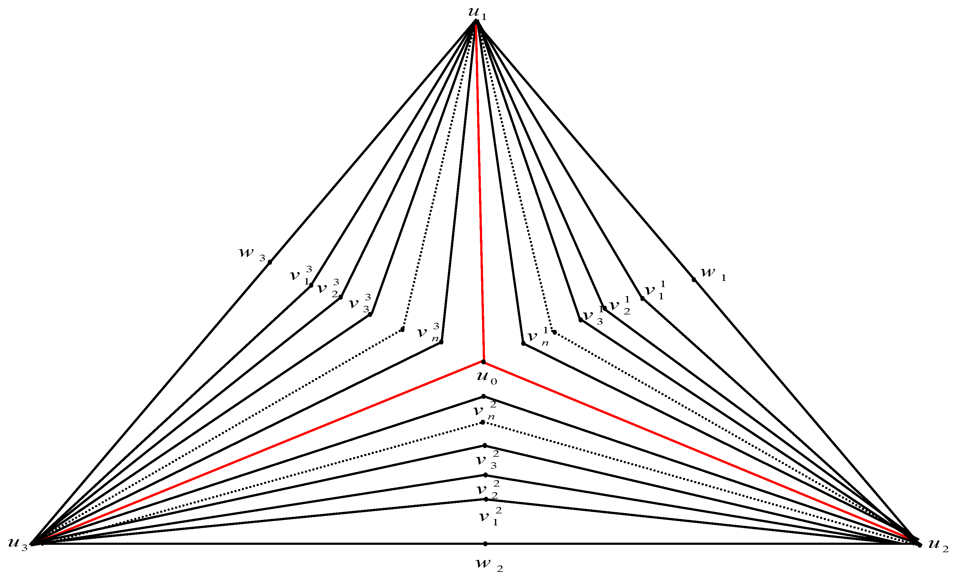
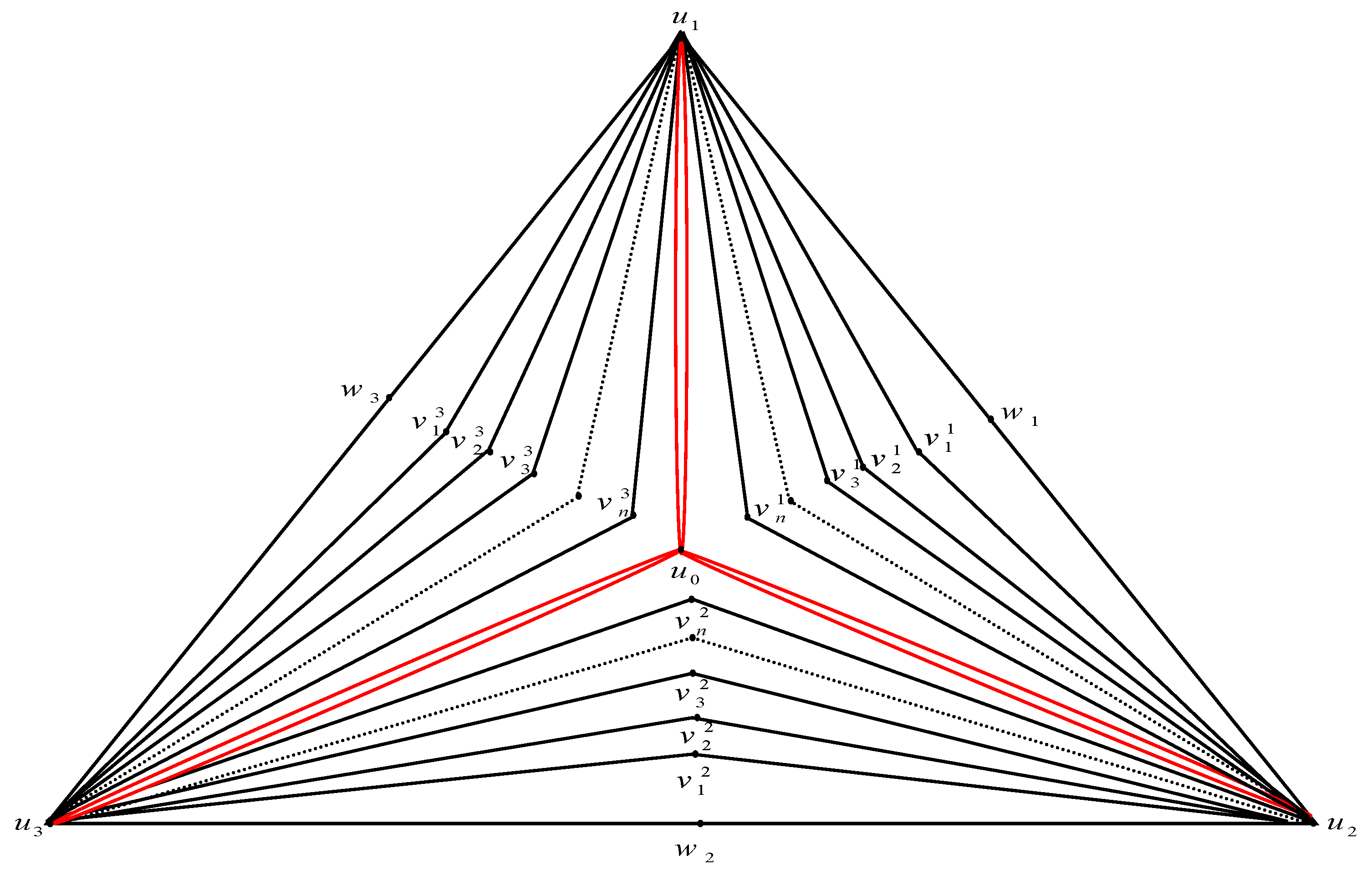
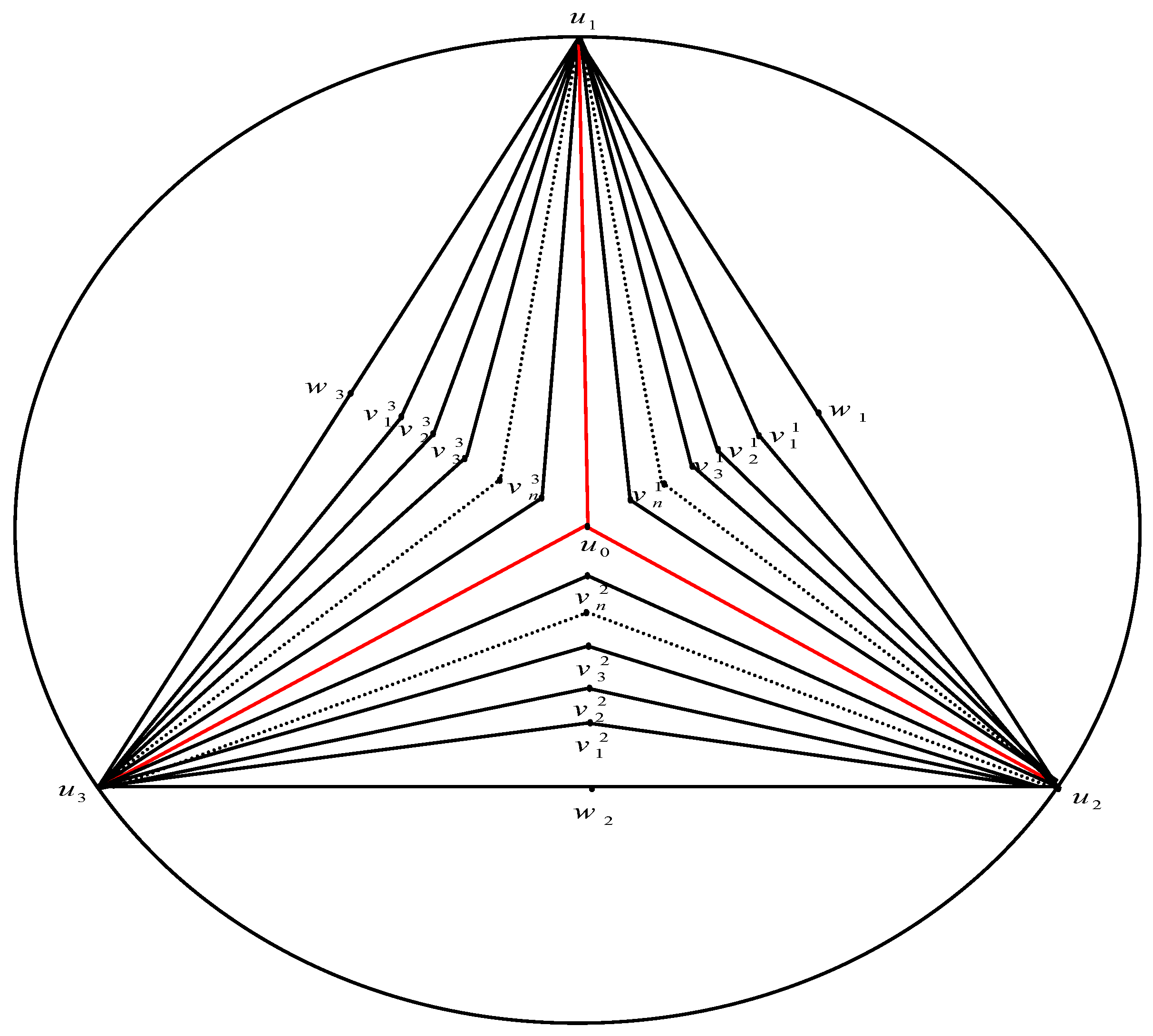
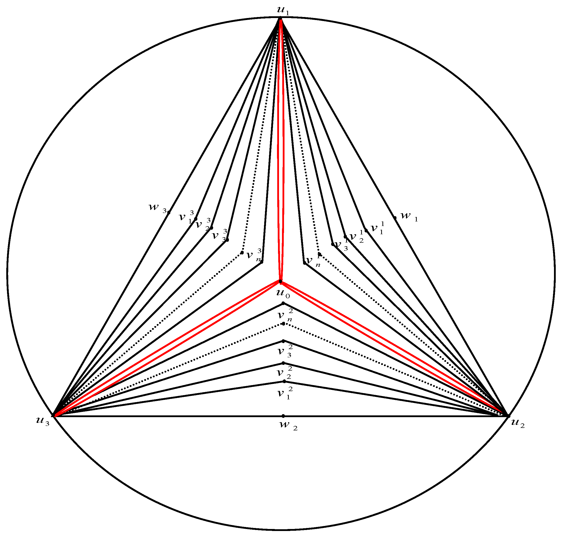
In this part we insert some relations regarding Chebyshev polynomials of the first and second types which we use in our calculations.

We start from their definitions, see Yuanping, et al. [20].

Let $A_n(x)$ be $n\times n$ matrix such that

$$A_n(x)=\left(\begin{array}{ccccc}2x& -1& 0& \cdots & 0\\ -1& 2x& -1& \ddots & ⋮\\ 0& \ddots & \ddots & \ddots & 0\\ ⋮& \ddots & \ddots & \ddots & -1\\ 0& \cdots & 0& -1& 2x\end{array}\right).$$

Furthermore, we render that the Chebyshev polynomials of the first type are defined by

$$T_n(x)=\cos (n{\cos }^{-1}x)$$

(1)

The Chebyshev polynomials of the second type are defined by

$$U_{n-1}(x)=\frac{1}{n}\frac{d}{dx}{T}_n(x)=\frac{\sin (n{\cos }^{-1}x)}{\sin ({\cos }^{-1}x)}$$

(2)

It is easily confirmed that

$$U_n(x)-2x{U}_{n-1}(x)+U_{n-2}(x)=0$$

(3)

It can then be shown from this recursion that by expanding $\det A_n(x)$ one obtains

$$U_n(x)=\det (A_n(x)),n\ge 1$$

(4)

Moreover, by solving the recursion (3), one gets the straightforward formula

$$U_n(x)=\frac{{(x+\sqrt{x^2-1})}^{n+1}-{(x-\sqrt{x^2-1})}^{n+1}}{2\sqrt{x^2-1}},n\ge 1,$$

(5)

where the conformity is valid for all complex $x$ (except at $x=\pm 1$, where the function can be taken as the limit).

The definition of $U_n(x)$ easily yields its zeros and it can therefore be confirmed that

$$U_{n-1}(x)=2^{n-1}{\displaystyle \prod _{j=1}^{n-1}(x-\cos \frac{j\pi }{n})}$$

(6)

One further notes that

$$U_{n-1}(-x)={(-1)}^{n-1}{U}_{n-1}(x)$$

(7)

From Equations (6) and (7), we have:

$$U_{n-1}{}^2(x)=4^{n-1}{\displaystyle \prod _{j=1}^{n-1}(x^2-{\cos }^2\frac{j\pi }{n})}$$

(8)

Finally, straightforward manipulation of the above formula produces the following formula (9), which is highly beneficial to us later:

$$U_{n-1}{}^2(\sqrt{\frac{x+2}{4}})={\displaystyle \prod _{j=1}^{n-1}(x-2\cos \frac{2j\pi }{n})}$$

(9)

Moreover, one can see that

$$U_{n-1}{}^2(x)=\frac{1-T_{2n}(x)}{2(1-x^2)}=\frac{1-T_n(2x^2-1)}{2(1-x^2)}$$

(10)

$$T_n(x)=\frac{1}{2}[{(x+\sqrt{x^2-1})}^n+({(x-\sqrt{x^2-1})}^n]$$

(11)

Now we introduce the following important two Lemmas.

Lemma 2

[21]. Let $B_n(x)$ be $n\times n$ Circulant matrix such that

$$B_n(x)=\left(\begin{array}{cccccc}x& 0& 1& \cdots & 1& 0\\ 0& \ddots & \ddots & \ddots & \ddots & 1\\ 1& \ddots & \ddots & \ddots & \ddots & ⋮\\ ⋮& \ddots & \ddots & \ddots & \ddots & 1\\ 1& \ddots & \ddots & \ddots & \ddots & 0\\ 0& 1& \cdots & 1& 0& x\end{array}\right).$$

Then for$n\ge 3,x\ge 4,$one has

$$\det (B_n(x))=\frac{2(x+n-3)}{x-3}[T_n(\frac{x-1}{2})-1].$$

Lemma 3

[22]. If $A\in F^{n\times n}$, $B\in F^{n\times m}$, $C\in F^{m\times n}$ and $D\in F^{m\times m}$. Suppose that $A$ and $D$ are nonsingular matrices, then:

$$\det \left(\begin{array}{cc}A& B\\ C& D\end{array}\right)=\det (A-B{D}^{-1}C)\det D=\det A\det (D-C{A}^{-1}B).$$

This Lemma gives a type of symmetry for some matrices which simplify our calculations of the complexity of graphs studied in this paper.

3. Main Results

Definition 1.

The pyramid graph$A_n^{(m)}$is the graph created from the gear graph$G_{m+1}$with vertices$\{u_0;u_1,u_2,\dots ,u_m;w_1,w_2,\dots ,w_m\}$and$m$sets of vertices, say,$\{v_1^1,v_2^1,\dots ,v_n^1\},\{v_1^2,v_2^2,\dots ,v_n^2\},\dots ,\{v_1^m,v_2^m,\dots ,v_n^m\},$such that for all$i=1,2,\dots ,n$the vertex$v_i^j$is adjacent to$u_j$and$u_{j+1}$,where$j=1,2,\dots ,m-1,$and$v_i^m$is adjacent to$u_1$and$u_m.$See Figure 1.

Figure 1. The pyramid graph $A_n^{(3)}$.

Theorem 1.

For$n\ge 0,m\ge 3,$$\tau (A_n^{(m)})=2^{mn}[{(n+2+\sqrt{2n+3})}^m+{(n+2-\sqrt{2n+3})}^m-2{(n+1)}^m].$

Proof. 

Using Lemma 1, we have

$$\tau (A_n^{(m)})=\frac{1}{{(mn+2m+1)}^2}\times \det ((mn+2m+1)I-D^c+A^c)=\frac{1}{{(mn+2m+1)}^2}\times$$

$$det\left(\begin{array}{cccccccccccccccccccccccccccccc}(m+1)& 0& 0& \cdots & \cdots & \cdots & 0& 1& \cdots & \cdots & \cdots & \cdots & 1& 1& \cdots & \cdots & \cdots & \cdots & \cdots & \cdots & \cdots & \cdots & \cdots & \cdots & \cdots & \cdots & \cdots & \cdots & \cdots & 1\\ 0& 2(n+2)& 1& \cdots & \cdots & \cdots & 1& 0& 1& \cdots & \cdots & 1& 0& 0& \cdots & 0& 1& \cdots & 1& \cdots & \cdots & 1& \cdots & 1& 1& \cdots & 1& 0& \cdots & 0\\ ⋮& 1& \ddots & \ddots & \ddots & \ddots & ⋮& 0& \ddots & \ddots & \ddots & \ddots & 1& 0& \cdots & 0& 0& \cdots & 0& 1& \cdots & 1& \cdots & \cdots & 1& \cdots & 1& 1& \cdots & 1\\ ⋮& ⋮& \ddots & \ddots & \ddots & \ddots & ⋮& 1& \ddots & \ddots & \ddots & ⋮& ⋮& 1& \cdots & 1& 0& \cdots & 0& 0& \cdots & 0& 1& \cdots & 1& \cdots & \cdots & 1& \cdots & 1\\ ⋮& ⋮& \ddots & \ddots & \ddots & \ddots & ⋮& ⋮& \ddots & \ddots & \ddots & ⋮& ⋮& 1& \cdots & 1& 1& \cdots & 1& 0& \cdots & 0& 0& \cdots & 0& 1& \cdots & 1& \cdots & \cdots \\ ⋮& ⋮& \ddots & \ddots & \ddots & \ddots & 1& ⋮& \ddots & \ddots & \ddots & \ddots & 1& ⋮& \cdots & \cdots & \cdots & \cdots & \cdots & \cdots & \cdots & \cdots & \cdots & \cdots & \cdots & \cdots & \cdots & \cdots & \cdots & ⋮\\ 0& 1& \cdots & \cdots & \cdots & 1& 2(n+2)& 1& \cdots & \cdots & 1& 0& 0& 1& \cdots & 1& 1& \cdots & 1& \cdots & \cdots & 1& \cdots & 1& 0& \cdots & 0& 0& \cdots & 0\\ 1& 0& 0& 1& \cdots & \cdots & 1& 3& 1& \cdots & \cdots & \cdots & 1& 1& \cdots & 1& 1& \cdots & 1& \cdots & \cdots & \cdots & \cdots & \cdots & 1& \cdots & 1& 1& \cdots & 1\\ ⋮& 1& \ddots & \ddots & \ddots & \ddots & ⋮& 1& \ddots & \ddots & \ddots & \ddots & ⋮& 1& \cdots & 1& 1& \cdots & 1& \cdots & \cdots & \cdots & \cdots & \cdots & 1& \cdots & 1& 1& \cdots & 1\\ ⋮& ⋮& \ddots & \ddots & \ddots & \ddots & ⋮& ⋮& \ddots & \ddots & \ddots & \ddots & ⋮& ⋮& \cdots & ⋮& ⋮& \cdots & ⋮& \cdots & \cdots & \cdots & \cdots & \cdots & ⋮& \cdots & ⋮& ⋮& \cdots & 1\\ ⋮& ⋮& \ddots & \ddots & \ddots & \ddots & 1& ⋮& \ddots & \ddots & \ddots & \ddots & ⋮& ⋮& \cdots & ⋮& ⋮& \cdots & ⋮& \cdots & \cdots & \cdots & \cdots & \cdots & ⋮& \cdots & ⋮& ⋮& \cdots & ⋮\\ ⋮& 1& \ddots & \ddots & \ddots & \ddots & 0& ⋮& \ddots & \ddots & \ddots & \ddots & ⋮& 1& \cdots & 1& 1& \cdots & 1& \cdots & \cdots & \cdots & \cdots & \cdots & 1& \cdots & 1& 1& \cdots & 1\\ 1& 0& 1& \cdots & \cdots & 1& 0& 1& \cdots & \cdots & \cdots & 1& 3& 1& \cdots & 1& 1& \cdots & 1& \cdots & \cdots & \cdots & \cdots & \cdots & 1& \cdots & 1& 1& \cdots & 1\\ 1& 0& 0& 1& \cdots & 1& 0& 1& 1& \cdots & \cdots & 1& 1& 3& 1& \cdots & \cdots & \cdots & \cdots & \cdots & \cdots & \cdots & \cdots & \cdots & \cdots & \cdots & \cdots & \cdots & \cdots & 1\\ ⋮& ⋮& ⋮& ⋮& ⋮& ⋮& ⋮& ⋮& ⋮& ⋮& ⋮& ⋮& ⋮& 1& \ddots & \ddots & \ddots & \ddots & \ddots & \ddots & \ddots & \ddots & \ddots & \ddots & \ddots & \ddots & \ddots & \ddots & \ddots & ⋮\\ ⋮& 0& 0& 1& ⋮& 1& ⋮& 1& 1& \cdots & \cdots & 1& 1& ⋮& \ddots & \ddots & \ddots & \ddots & \ddots & \ddots & \ddots & \ddots & \ddots & \ddots & \ddots & \ddots & \ddots & \ddots & \ddots & ⋮\\ ⋮& 1& 0& 0& ⋮& 1& ⋮& 1& 1& \cdots & \cdots & 1& 1& ⋮& \ddots & \ddots & \ddots & \ddots & \ddots & \ddots & \ddots & \ddots & \ddots & \ddots & \ddots & \ddots & \ddots & \ddots & \ddots & ⋮\\ ⋮& ⋮& ⋮& ⋮& ⋮& ⋮& ⋮& ⋮& ⋮& ⋮& ⋮& ⋮& ⋮& ⋮& \ddots & \ddots & \ddots & \ddots & \ddots & \ddots & \ddots & \ddots & \ddots & \ddots & \ddots & \ddots & \ddots & \ddots & \ddots & ⋮\\ ⋮& 1& 0& 0& ⋮& 1& ⋮& 1& 1& \cdots & \cdots & 1& 1& ⋮& \ddots & \ddots & \ddots & \ddots & \ddots & \ddots & \ddots & \ddots & \ddots & \ddots & \ddots & \ddots & \ddots & \ddots & \ddots & ⋮\\ ⋮& 1& 1& 0& ⋮& ⋮& ⋮& ⋮& ⋮& ⋮& ⋮& ⋮& ⋮& ⋮& \ddots & \ddots & \ddots & \ddots & \ddots & \ddots & \ddots & \ddots & \ddots & \ddots & \ddots & \ddots & \ddots & \ddots & \ddots & ⋮\\ ⋮& ⋮& ⋮& ⋮& ⋮& ⋮& ⋮& ⋮& ⋮& ⋮& ⋮& ⋮& ⋮& ⋮& \ddots & \ddots & \ddots & \ddots & \ddots & \ddots & \ddots & \ddots & \ddots & \ddots & \ddots & \ddots & \ddots & \ddots & \ddots & ⋮\\ ⋮& 1& 1& 0& ⋮& 1& ⋮& ⋮& ⋮& ⋮& ⋮& ⋮& ⋮& ⋮& \ddots & \ddots & \ddots & \ddots & \ddots & \ddots & \ddots & \ddots & \ddots & \ddots & \ddots & \ddots & \ddots & \ddots & \ddots & ⋮\\ ⋮& ⋮& ⋮& 1& ⋮& ⋮& ⋮& ⋮& ⋮& ⋮& ⋮& ⋮& ⋮& ⋮& \ddots & \ddots & \ddots & \ddots & \ddots & \ddots & \ddots & \ddots & \ddots & \ddots & \ddots & \ddots & \ddots & \ddots & \ddots & ⋮\\ ⋮& ⋮& ⋮& ⋮& ⋮& 1& ⋮& ⋮& ⋮& ⋮& ⋮& ⋮& ⋮& ⋮& \ddots & \ddots & \ddots & \ddots & \ddots & \ddots & \ddots & \ddots & \ddots & \ddots & \ddots & \ddots & \ddots & \ddots & \ddots & ⋮\\ ⋮& 1& 1& 1& ⋮& 0& ⋮& ⋮& ⋮& ⋮& ⋮& ⋮& ⋮& ⋮& \ddots & \ddots & \ddots & \ddots & \ddots & \ddots & \ddots & \ddots & \ddots & \ddots & \ddots & \ddots & \ddots & \ddots & \ddots & ⋮\\ ⋮& ⋮& ⋮& ⋮& ⋮& ⋮& ⋮& ⋮& ⋮& ⋮& ⋮& ⋮& ⋮& ⋮& \ddots & \ddots & \ddots & \ddots & \ddots & \ddots & \ddots & \ddots & \ddots & \ddots & \ddots & \ddots & \ddots & \ddots & \ddots & ⋮\\ ⋮& 1& 1& ⋮& ⋮& 0& ⋮& 1& 1& \cdots & \cdots & 1& 1& ⋮& \ddots & \ddots & \ddots & \ddots & \ddots & \ddots & \ddots & \ddots & \ddots & \ddots & \ddots & \ddots & \ddots & \ddots & \ddots & ⋮\\ ⋮& 0& 1& 1& ⋮& 0& ⋮& 1& 1& \cdots & \cdots & 1& 1& ⋮& \ddots & \ddots & \ddots & \ddots & \ddots & \ddots & \ddots & \ddots & \ddots & \ddots & \ddots & \ddots & \ddots & \ddots & \ddots & ⋮\\ ⋮& ⋮& ⋮& ⋮& ⋮& ⋮& ⋮& ⋮& ⋮& ⋮& ⋮& ⋮& ⋮& ⋮& \ddots & \ddots & \ddots & \ddots & \ddots & \ddots & \ddots & \ddots & \ddots & \ddots & \ddots & \ddots & \ddots & \ddots & \ddots & 1\\ 1& 0& 1& 1& \cdots & 0& \cdots & 1& 1& \cdots & \cdots & 1& 1& 1& \cdots & \cdots & \cdots & \cdots & \cdots & \cdots & \cdots & \cdots & \cdots & \cdots & \cdots & \cdots & \cdots & \cdots & 1& 3\end{array}\right)$$

Let $j=(1\cdots 1)$ be the $1\times n$ matrix with all one, and $J_n$ be the $n\times n$ matrix with all one. Set $a=2n+4$ and $b=mn+2m+1$. Then we obtain:

$$\tau \left(A_n^{\left(m\right)}\right)=\frac{1}{b^2}\times det\left(\begin{array}{ccccccccccccccccccc}m+1& 0& \cdots & \cdots & \cdots & \cdots & 0& 1& \cdots & \cdots & \cdots & \cdots & 1& j& \cdots & \cdots & \cdots & \cdots & j\\ 0& a& 1& \cdots & \cdots & \cdots & 1& 0& 1& \cdots & \cdots & 1& 0& 0& j& \cdots & \cdots & j& 0\\ ⋮& 1& \ddots & \ddots & \ddots & \ddots & ⋮& 0& 0& \ddots & \ddots & \ddots & 1& 0& \ddots & \ddots & \ddots & \ddots & j\\ ⋮& ⋮& \ddots & \ddots & \ddots & \ddots & ⋮& 1& 0& \ddots & \ddots & \ddots & ⋮& j& \ddots & \ddots & \ddots & \ddots & ⋮\\ ⋮& ⋮& \ddots & \ddots & \ddots & \ddots & ⋮& ⋮& \ddots & \ddots & \ddots & \ddots & ⋮& ⋮& \ddots & \ddots & \ddots & \ddots & ⋮\\ ⋮& ⋮& \ddots & \ddots & \ddots & \ddots & 1& ⋮& \ddots & \ddots & 0& 0& 1& ⋮& \ddots & \ddots & \ddots & \ddots & j\\ 0& 1& \cdots & \cdots & \cdots & 1& a& 1& \cdots & \cdots & 1& 0& 0& j& \cdots & \cdots & j& 0& 0\\ 1& 0& 0& 1& \cdots & \cdots & 1& 3& 1& \cdots & \cdots & \cdots & 1& j& \cdots & \cdots & \cdots & \cdots & j\\ ⋮& 1& 0& \ddots & \ddots & \ddots & 1& 1& \ddots & \ddots & \ddots & \ddots & ⋮& ⋮& \ddots & \ddots & \ddots & \ddots & ⋮\\ ⋮& ⋮& \ddots & \ddots & \ddots & \ddots & ⋮& ⋮& \ddots & \ddots & \ddots & \ddots & ⋮& ⋮& \ddots & \ddots & \ddots & \ddots & ⋮\\ ⋮& ⋮& \ddots & \ddots & \ddots & \ddots & 1& ⋮& \ddots & \ddots & \ddots & \ddots & ⋮& ⋮& \ddots & \ddots & \ddots & \ddots & ⋮\\ ⋮& 1& \ddots & \ddots & \ddots & \ddots & 0& ⋮& \ddots & \ddots & \ddots & \ddots & 1& ⋮& \ddots & \ddots & \ddots & \ddots & ⋮\\ 1& 0& 1& \cdots & \cdots & 1& 0& 1& \cdots & \cdots & \cdots & 1& 3& j& \cdots & \cdots & \cdots & \cdots & j\\ j^t& 0& 0& j^t& \cdots & \cdots & j^t& j^t& \cdots & \cdots & \cdots & \cdots & j^t& & & & & & \\ ⋮& j^t& 0& \ddots & \ddots & \ddots & ⋮& ⋮& \ddots & \ddots & \ddots & \ddots & ⋮& & & & & & \\ ⋮& ⋮& \ddots & \ddots & \ddots & \ddots & ⋮& ⋮& \ddots & \ddots & \ddots & \ddots & ⋮& & & 2I_{mn}+J_{mn}& & & \\ ⋮& ⋮& \ddots & \ddots & \ddots & \ddots & j^t& ⋮& \ddots & \ddots & \ddots & \ddots & ⋮& & & & & & \\ ⋮& j^t& \ddots & \ddots & \ddots & \ddots & 0& ⋮& \ddots & \ddots & \ddots & \ddots & ⋮& & & & & & \\ j^t& 0& j^t& \cdots & \cdots & j^t& 0& j^t& \cdots & \cdots & \cdots & \cdots & j^t& & & & & & \end{array}\right)$$

$$=\frac{1}{b^2}\times det\left(\begin{array}{ccccccccccccccccccc}b& 0& \cdots & \cdots & \cdots & \cdots & 0& 1& \cdots & \cdots & \cdots & \cdots & 1& j& \cdots & \cdots & \cdots & \cdots & j\\ b& a& 1& \cdots & \cdots & \cdots & 1& 0& 1& \cdots & \cdots & 1& 0& 0& j& \cdots & \cdots & j& 0\\ ⋮& 1& \ddots & \ddots & \ddots & \ddots & ⋮& 0& 0& \ddots & \ddots & \ddots & 1& 0& \ddots & \ddots & \ddots & \ddots & j\\ ⋮& ⋮& \ddots & \ddots & \ddots & \ddots & ⋮& 1& 0& \ddots & \ddots & \ddots & ⋮& j& \ddots & \ddots & \ddots & \ddots & ⋮\\ ⋮& ⋮& \ddots & \ddots & \ddots & \ddots & ⋮& ⋮& \ddots & \ddots & \ddots & \ddots & ⋮& ⋮& \ddots & \ddots & \ddots & \ddots & ⋮\\ ⋮& ⋮& \ddots & \ddots & \ddots & \ddots & 1& ⋮& \ddots & \ddots & 0& 0& 1& ⋮& \ddots & \ddots & \ddots & \ddots & j\\ b& 1& \cdots & \cdots & \cdots & 1& a& 1& \cdots & \cdots & 1& 0& 0& j& \cdots & \cdots & j& 0& 0\\ b& 0& 0& 1& \cdots & \cdots & 1& 3& 1& \cdots & \cdots & \cdots & 1& j& \cdots & \cdots & \cdots & \cdots & j\\ ⋮& 1& 0& \ddots & \ddots & \ddots & 1& 1& \ddots & \ddots & \ddots & \ddots & ⋮& ⋮& \ddots & \ddots & \ddots & \ddots & ⋮\\ ⋮& ⋮& \ddots & \ddots & \ddots & \ddots & ⋮& ⋮& \ddots & \ddots & \ddots & \ddots & ⋮& ⋮& \ddots & \ddots & \ddots & \ddots & ⋮\\ ⋮& ⋮& \ddots & \ddots & \ddots & \ddots & 1& ⋮& \ddots & \ddots & \ddots & \ddots & ⋮& ⋮& \ddots & \ddots & \ddots & \ddots & ⋮\\ ⋮& 1& \ddots & \ddots & \ddots & \ddots & 0& ⋮& \ddots & \ddots & \ddots & \ddots & 1& ⋮& \ddots & \ddots & \ddots & \ddots & ⋮\\ b& 0& 1& \cdots & \cdots & 1& 0& 1& \cdots & \cdots & \cdots & 1& 3& j& \cdots & \cdots & \cdots & \cdots & j\\ b{j}^t& 0& 0& j^t& \cdots & \cdots & j^t& j^t& \cdots & \cdots & \cdots & \cdots & j^t& & & & & & \\ ⋮& j^t& 0& \ddots & \ddots & \ddots & ⋮& ⋮& \ddots & \ddots & \ddots & \ddots & ⋮& & & & & & \\ ⋮& ⋮& \ddots & \ddots & \ddots & \ddots & ⋮& ⋮& \ddots & \ddots & \ddots & \ddots & ⋮& & & 2I_{mn}+J_{mn}& & & \\ ⋮& ⋮& \ddots & \ddots & \ddots & \ddots & j^t& ⋮& \ddots & \ddots & \ddots & \ddots & ⋮& & & & & & \\ ⋮& j^t& \ddots & \ddots & \ddots & \ddots & 0& ⋮& \ddots & \ddots & \ddots & \ddots & ⋮& & & & & & \\ b{j}^t& 0& j^t& \cdots & \cdots & j^t& 0& j^t& \cdots & \cdots & \cdots & \cdots & j^t& & & & & & \end{array}\right)$$

$$=\frac{1}{b}\times det\left(\begin{array}{ccccccccccccccccccc}1& 0& \cdots & \cdots & \cdots & \cdots & 0& 1& \cdots & \cdots & \cdots & \cdots & 1& j& \cdots & \cdots & \cdots & \cdots & j\\ 1& a& 1& \cdots & \cdots & \cdots & 1& 0& 1& \cdots & \cdots & 1& 0& 0& j& \cdots & \cdots & j& 0\\ ⋮& 1& \ddots & \ddots & \ddots & \ddots & ⋮& 0& 0& \ddots & \ddots & \ddots & 1& 0& \ddots & \ddots & \ddots & \ddots & j\\ ⋮& ⋮& \ddots & \ddots & \ddots & \ddots & ⋮& 1& 0& \ddots & \ddots & \ddots & ⋮& j& \ddots & \ddots & \ddots & \ddots & ⋮\\ ⋮& ⋮& \ddots & \ddots & \ddots & \ddots & ⋮& ⋮& \ddots & \ddots & \ddots & \ddots & ⋮& ⋮& \ddots & \ddots & \ddots & \ddots & ⋮\\ ⋮& ⋮& \ddots & \ddots & \ddots & \ddots & 1& ⋮& \ddots & \ddots & 0& 0& 1& ⋮& \ddots & \ddots & \ddots & \ddots & j\\ 1& 1& \cdots & \cdots & \cdots & 1& a& 1& \cdots & \cdots & 1& 0& 0& j& \cdots & \cdots & j& 0& 0\\ 1& 0& 0& 1& \cdots & \cdots & 1& 3& 1& \cdots & \cdots & \cdots & 1& j& \cdots & \cdots & \cdots & \cdots & j\\ ⋮& 1& 0& \ddots & \ddots & \ddots & 1& 1& \ddots & \ddots & \ddots & \ddots & ⋮& ⋮& \ddots & \ddots & \ddots & \ddots & ⋮\\ ⋮& ⋮& \ddots & \ddots & \ddots & \ddots & ⋮& ⋮& \ddots & \ddots & \ddots & \ddots & ⋮& ⋮& \ddots & \ddots & \ddots & \ddots & ⋮\\ ⋮& ⋮& \ddots & \ddots & \ddots & \ddots & 1& ⋮& \ddots & \ddots & \ddots & \ddots & ⋮& ⋮& \ddots & \ddots & \ddots & \ddots & ⋮\\ ⋮& 1& \ddots & \ddots & \ddots & \ddots & 0& ⋮& \ddots & \ddots & \ddots & \ddots & 1& ⋮& \ddots & \ddots & \ddots & \ddots & ⋮\\ 1& 0& 1& \cdots & \cdots & 1& 0& 1& \cdots & \cdots & \cdots & 1& 3& j& \cdots & \cdots & \cdots & \cdots & j\\ 1j^t& 0& 0& j^t& \cdots & \cdots & j^t& j^t& \cdots & \cdots & \cdots & \cdots & j^t& & & & & & \\ ⋮& j^t& 0& \ddots & \ddots & \ddots & ⋮& ⋮& \ddots & \ddots & \ddots & \ddots & ⋮& & & & & & \\ ⋮& ⋮& \ddots & \ddots & \ddots & \ddots & ⋮& ⋮& \ddots & \ddots & \ddots & \ddots & ⋮& & & 2I_{mn}+J_{mn}& & & \\ ⋮& ⋮& \ddots & \ddots & \ddots & \ddots & j^t& ⋮& \ddots & \ddots & \ddots & \ddots & ⋮& & & & & & \\ ⋮& j^t& \ddots & \ddots & \ddots & \ddots & 0& ⋮& \ddots & \ddots & \ddots & \ddots & ⋮& & & & & & \\ 1j^t& 0& j^t& \cdots & \cdots & j^t& 0& j^t& \cdots & \cdots & \cdots & \cdots & j^t& & & & & & \end{array}\right)$$

$$=\frac{1}{b}\times det\left(\begin{array}{ccccccccccccccccccc}1& 0& \cdots & \cdots & \cdots & \cdots & 0& 1& \cdots & \cdots & \cdots & \cdots & 1& j& \cdots & \cdots & \cdots & \cdots & j\\ 0& a& 1& \cdots & \cdots & \cdots & 1& -1& 0& \cdots & \cdots & 0& -1& -j& 0& \cdots & \cdots & 0& -j\\ ⋮& 1& \ddots & \ddots & \ddots & \ddots & ⋮& -1& -1& \ddots & \ddots & \ddots & 0& -j& \ddots & \ddots & \ddots & \ddots & 0\\ ⋮& ⋮& \ddots & \ddots & \ddots & \ddots & ⋮& 0& \ddots & \ddots & \ddots & \ddots & ⋮& 0& \ddots & \ddots & \ddots & \ddots & ⋮\\ ⋮& ⋮& \ddots & \ddots & \ddots & \ddots & ⋮& ⋮& \ddots & \ddots & \ddots & \ddots & ⋮& ⋮& \ddots & \ddots & \ddots & \ddots & ⋮\\ ⋮& ⋮& \ddots & \ddots & \ddots & \ddots & 1& ⋮& \ddots & \ddots & \ddots & -1& 0& ⋮& \ddots & \ddots & \ddots & \ddots & 0\\ 0& 1& \cdots & \cdots & \cdots & 1& a& 0& \cdots & \cdots & 0& -1& -1& 0& \cdots & \cdots & 0& -j& -j\\ 0& 0& 0& 1& \cdots & \cdots & 1& 2& 0& \cdots & \cdots & \cdots & 0& 0& \cdots & \cdots & \cdots & \cdots & 0\\ ⋮& 1& 0& \ddots & \ddots & \ddots & 1& 0& \ddots & \ddots & \ddots & \ddots & ⋮& ⋮& \ddots & \ddots & \ddots & \ddots & ⋮\\ ⋮& ⋮& \ddots & \ddots & \ddots & \ddots & ⋮& ⋮& \ddots & \ddots & \ddots & \ddots & ⋮& ⋮& \ddots & \ddots & \ddots & \ddots & ⋮\\ ⋮& ⋮& \ddots & \ddots & \ddots & \ddots & 1& ⋮& \ddots & \ddots & \ddots & \ddots & ⋮& ⋮& \ddots & \ddots & \ddots & \ddots & ⋮\\ ⋮& 1& \ddots & \ddots & \ddots & \ddots & 0& ⋮& \ddots & \ddots & \ddots & \ddots & 0& ⋮& \ddots & \ddots & \ddots & \ddots & ⋮\\ 0& 0& 1& \cdots & \cdots & 1& 0& 0& \cdots & \cdots & \cdots & 0& 2& 0& \cdots & \cdots & \cdots & \cdots & 0\\ 0& 0& 0& j^t& \cdots & \cdots & j^t& 0& \cdots & \cdots & \cdots & \cdots & 0& & & & & & \\ ⋮& j^t& 0& \ddots & \ddots & \ddots & ⋮& ⋮& \ddots & \ddots & \ddots & \ddots & ⋮& & & & & & \\ ⋮& ⋮& \ddots & \ddots & \ddots & \ddots & ⋮& ⋮& \ddots & \ddots & \ddots & \ddots & ⋮& & & 2I_{mn}& & & \\ ⋮& ⋮& \ddots & \ddots & \ddots & \ddots & j^t& ⋮& \ddots & \ddots & \ddots & \ddots & ⋮& & & & & & \\ ⋮& j^t& \ddots & \ddots & \ddots & \ddots & 0& ⋮& \ddots & \ddots & \ddots & \ddots & ⋮& & & & & & \\ 0& 0& j^t& \cdots & \cdots & j^t& 0& 0& \cdots & \cdots & \cdots & \cdots & 0& & & & & & \end{array}\right)$$

$$=\frac{1}{b}\times det\left(\begin{array}{cccccccccccccccccc}a& 1& \cdots & \cdots & \cdots & 1& -1& 0& \cdots & \cdots & 0& -1& -j& 0& \cdots & \cdots & 0& -j\\ 1& \ddots & \ddots & \ddots & \ddots & ⋮& -1& -1& \ddots & \ddots & \ddots & 0& -j& \ddots & \ddots & \ddots & \ddots & 0\\ ⋮& \ddots & \ddots & \ddots & \ddots & ⋮& 0& \ddots & \ddots & \ddots & \ddots & ⋮& 0& \ddots & \ddots & \ddots & \ddots & ⋮\\ ⋮& \ddots & \ddots & \ddots & \ddots & ⋮& ⋮& \ddots & \ddots & \ddots & \ddots & ⋮& ⋮& \ddots & \ddots & \ddots & \ddots & ⋮\\ ⋮& \ddots & \ddots & \ddots & \ddots & 1& ⋮& \ddots & \ddots & \ddots & -1& 0& ⋮& \ddots & \ddots & \ddots & \ddots & 0\\ 1& \cdots & \cdots & \cdots & 1& a& 0& \cdots & \cdots & 0& -1& -1& 0& \cdots & \cdots & 0& -j& -j\\ 0& 0& 1& \cdots & \cdots & 1& 2& 0& \cdots & \cdots & \cdots & 0& 0& \cdots & \cdots & \cdots & \cdots & 0\\ 1& 0& \ddots & \ddots & \ddots & 1& 0& \ddots & \ddots & \ddots & \ddots & ⋮& ⋮& \ddots & \ddots & \ddots & \ddots & ⋮\\ ⋮& \ddots & \ddots & \ddots & \ddots & ⋮& ⋮& \ddots & \ddots & \ddots & \ddots & ⋮& ⋮& \ddots & \ddots & \ddots & \ddots & ⋮\\ ⋮& \ddots & \ddots & \ddots & \ddots & 1& ⋮& \ddots & \ddots & \ddots & \ddots & ⋮& ⋮& \ddots & \ddots & \ddots & \ddots & ⋮\\ 1& \ddots & \ddots & \ddots & \ddots & 0& ⋮& \ddots & \ddots & \ddots & \ddots & 0& ⋮& \ddots & \ddots & \ddots & \ddots & ⋮\\ 0& 1& \cdots & \cdots & 1& 0& 0& \cdots & \cdots & \cdots & 0& 2& 0& \cdots & \cdots & \cdots & \cdots & 0\\ 0& 0& j^t& \cdots & \cdots & j^t& 0& \cdots & \cdots & \cdots & \cdots & 0& & & & & & \\ j^t& 0& \ddots & \ddots & \ddots & ⋮& ⋮& \ddots & \ddots & \ddots & \ddots & ⋮& & & & & & \\ ⋮& \ddots & \ddots & \ddots & \ddots & ⋮& ⋮& \ddots & \ddots & \ddots & \ddots & ⋮& & & 2I_{mn}& & & \\ ⋮& \ddots & \ddots & \ddots & \ddots & j^t& ⋮& \ddots & \ddots & \ddots & \ddots & ⋮& & & & & & \\ j^t& \ddots & \ddots & \ddots & \ddots & 0& ⋮& \ddots & \ddots & \ddots & \ddots & ⋮& & & & & & \\ 0& j^t& \cdots & \cdots & j^t& 0& 0& \cdots & \cdots & \cdots & \cdots & 0& & & & & & \end{array}\right)$$

Using Lemma 3, yields

$$\tau (A_n^{(m)})=\frac{1}{b}\times \det \left(\begin{array}{cc}A& B\\ C& 2I_{mn}\end{array}\right)=\frac{1}{b}\times \det (A-B\frac{1}{2I_{mn}}C)\times 2^{mn}$$

$$=\frac{1}{b}{2}^{mn}\times 2^{-2m}\times det\left(\begin{array}{cccccccccccc}2a& n+2& 2(n+1)& \cdots & 2(n+1)& n+2& -2& 0& \cdots & \cdots & 0& -2\\ n+2& 2a& n+2& 2(n+1)& \cdots & 2(n+1)& -2& \ddots & \ddots & \ddots & \ddots & 0\\ 2(n+1)& n+2& \ddots & \ddots & \ddots & ⋮& 0& \ddots & \ddots & \ddots & \ddots & ⋮\\ ⋮& \ddots & \ddots & \ddots & \ddots & 2(n+1)& ⋮& \ddots & \ddots & \ddots & \ddots & ⋮\\ 2(n+1)& \ddots & \ddots & \ddots & \ddots & n+2& ⋮& \ddots & \ddots & \ddots & \ddots & 0\\ n+2& 2(n+1)& \cdots & 2(n+1)& n+2& 2a& 0& \cdots & \cdots & 0& -2& -2\\ 0& 0& 2& \cdots & \cdots & 2& 4& 0& \cdots & \cdots & \cdots & 0\\ 2& \ddots & \ddots & \ddots & \ddots & ⋮& 0& \ddots & \ddots & \ddots & \ddots & ⋮\\ ⋮& \ddots & \ddots & \ddots & \ddots & ⋮& ⋮& \ddots & \ddots & \ddots & \ddots & ⋮\\ ⋮& \ddots & \ddots & \ddots & \ddots & 2& ⋮& \ddots & \ddots & \ddots & \ddots & ⋮\\ 2& \ddots & \ddots & \ddots & \ddots & 0& ⋮& \ddots & \ddots & \ddots & \ddots & 0\\ 0& 2& \cdots & \cdots & 2& 0& 0& \cdots & \cdots & \cdots & 0& 4\end{array}\right)$$

Using Lemma 3 again, yields

$$\tau (A_n^{(m)})=\frac{2^{mn-2m}}{b}\times \det \left(\begin{array}{cc}D& E\\ F& 4I_m\end{array}\right)=\frac{2^{mn}}{b}\times \det (D-E\frac{1}{4I_m}F)$$

$$\tau (A_n^{(m)})=\frac{2^{mn}}{b}\times \det \left(\begin{array}{cccccc}2a& (n+3)& 2(n+2)& \cdots & 2(n+2)& (n+3)\\ (n+3)& 2a& (n+3)& \ddots & \cdots & 2(n+2)\\ 2(n+2)& \ddots & \ddots & \ddots & \ddots & ⋮\\ ⋮& \ddots & \ddots & \ddots & \ddots & 2(n+2)\\ 2(n+2)& \ddots & \ddots & \ddots & \ddots & (n+3)\\ (n+3)& 2(n+2)& \cdots & 2(n+2)& (n+3)& 2a\end{array}\right)$$

Straightforward inducement using the properties of determinants, one can obtain

$$\tau (A_n^{(m)})=\frac{2^{mn}}{b}\times \frac{2b}{mn+m+2}\times \det \left(\begin{array}{cccccc}(2a-n-3)& 0& (n+1)& \cdots & (n+1)& 0\\ 0& (2a-n-3)& 0& \ddots & \cdots & (n+1)\\ (n+1)& \ddots & \ddots & \ddots & \ddots & ⋮\\ ⋮& \ddots & \ddots & \ddots & \ddots & (n+1)\\ (n+1)& \ddots & \ddots & \ddots & \ddots & 0\\ 0& (n+1)& \cdots & (n+1)& 0& (2a-n-3)\end{array}\right)$$

$$=\frac{2^{mn+1}{(n+1)}^m}{mn+m+2}\times \det \left(\begin{array}{cccccc}\frac{(2a-n-3)}{(n+1)}& 0& 1& \cdots & 1& 0\\ 0& \frac{(2a-n-3)}{(n+1)}& 0& \ddots & \ddots & 1\\ 1& \ddots & \ddots & \ddots & \ddots & ⋮\\ ⋮& \ddots & \ddots & \ddots & \ddots & 1\\ 1& \ddots & \ddots & \ddots & \ddots & 0\\ 0& 1& \cdots & 1& 0& \frac{(2a-n-3)}{(n+1)}\end{array}\right)$$

Using Lemma 2, yields

$$\begin{gathered} \tau (A_n^{(m)})=2^{mn+1}\times \frac{{(n+1)}^m}{mn+m+2}\times \frac{2(\frac{2a-n-3}{n+1}+m-3)}{\frac{2a-n-3}{n+1}-3}\times [T_m(\frac{\frac{2a-n-3}{n+1}-1}{2})-1] \\ =2^{mn+1}\times {(n+1)}^m\times [T_m(\frac{n+2}{n+1})-1]. \end{gathered}$$

Using Equation (11), yields the result. □

Definition 2.

The pyramid graph$B_n^{(m)}$is the graph created from the gear graph$G_{m+1}$with vertices$\{u_0;u_1,u_2,\dots ,u_m;w_1,w_2,\dots ,w_m\}$with double internal edges and$m$sets of vertices, say,$\{v_1^1,v_2^1,\dots ,v_n^1\},\{v_1^2,v_2^2,\dots ,v_n^2\},\dots ,\{v_1^m,v_2^m,\dots ,v_n^m\}$, such that for all$i=1,2,\dots ,n$the vertex$v_i^j$is adjacent to$u_j$and$u_{j+1}$, where$j=1,2,\dots ,m-1,$and$v_i^m$is adjacent to$u_1$and$u_m.$See Figure 2.

Figure 2. The pyramid graph $B_n^{(3)}$.

Theorem 2.

For$n\ge 0,m\ge 3,$$\tau (B_n^{(m)})=2^{mn}[{(n+3+2\sqrt{n+2})}^m+{(n+3-2\sqrt{n+2})}^m-2{(n+1)}^m].$

Proof. 

Using Lemma 1, we get:

$$\tau (B_n^{(m)})=\frac{1}{{(mn+2m+1)}^2}\times \det ((mn+2m+1)I-D^c+A^c)=\frac{1}{{(mn+2m+1)}^2}\times$$

$$det\left(\begin{array}{cccccccccccccccccccccccccccccc}(2m+1)& -1& -1& \cdots & \cdots & \cdots & -1& 1& \cdots & \cdots & \cdots & \cdots & 1& 1& \cdots & \cdots & \cdots & \cdots & \cdots & \cdots & \cdots & \cdots & \cdots & \cdots & \cdots & \cdots & \cdots & \cdots & \cdots & 1\\ -1& (2n+5)& 1& \cdots & \cdots & \cdots & 1& 0& 1& \cdots & \cdots & 1& 0& 0& \cdots & 0& 1& \cdots & 1& \cdots & \cdots & 1& \cdots & 1& 1& \cdots & 1& 0& \cdots & 0\\ ⋮& 1& \ddots & \ddots & \ddots & \ddots & ⋮& 0& \ddots & \ddots & \ddots & \ddots & 1& 0& \cdots & 0& 0& \cdots & 0& 1& \cdots & 1& \cdots & \cdots & 1& \cdots & 1& 1& \cdots & 1\\ ⋮& ⋮& \ddots & \ddots & \ddots & \ddots & ⋮& 1& \ddots & \ddots & \ddots & ⋮& ⋮& 1& \cdots & 1& 0& \cdots & 0& 0& \cdots & 0& 1& \cdots & 1& \cdots & \cdots & 1& \cdots & 1\\ ⋮& ⋮& \ddots & \ddots & \ddots & \ddots & ⋮& ⋮& \ddots & \ddots & \ddots & ⋮& ⋮& 1& \cdots & 1& 1& \cdots & 1& 0& \cdots & 0& 0& \cdots & 0& 1& \cdots & 1& \cdots & \cdots \\ ⋮& ⋮& \ddots & \ddots & \ddots & \ddots & 1& ⋮& \ddots & \ddots & \ddots & \ddots & 1& ⋮& \cdots & \cdots & \cdots & \cdots & \cdots & \cdots & \cdots & \cdots & \cdots & \cdots & \cdots & \cdots & \cdots & \cdots & \cdots & ⋮\\ -1& 1& \cdots & \cdots & \cdots & 1& (2n+5)& 1& \cdots & \cdots & 1& 0& 0& 1& \cdots & 1& 1& \cdots & 1& \cdots & \cdots & 1& \cdots & 1& 0& \cdots & 0& 0& \cdots & 0\\ 1& 0& 0& 1& \cdots & \cdots & 1& 3& 1& \cdots & \cdots & \cdots & 1& 1& \cdots & 1& 1& \cdots & 1& \cdots & \cdots & \cdots & \cdots & \cdots & 1& \cdots & 1& 1& \cdots & 1\\ ⋮& 1& \ddots & \ddots & \ddots & \ddots & ⋮& 1& \ddots & \ddots & \ddots & \ddots & ⋮& 1& \cdots & 1& 1& \cdots & 1& \cdots & \cdots & \cdots & \cdots & \cdots & 1& \cdots & 1& 1& \cdots & 1\\ ⋮& ⋮& \ddots & \ddots & \ddots & \ddots & ⋮& ⋮& \ddots & \ddots & \ddots & \ddots & ⋮& ⋮& \cdots & ⋮& ⋮& \cdots & ⋮& \cdots & \cdots & \cdots & \cdots & \cdots & ⋮& \cdots & ⋮& ⋮& \cdots & 1\\ ⋮& ⋮& \ddots & \ddots & \ddots & \ddots & 1& ⋮& \ddots & \ddots & \ddots & \ddots & ⋮& ⋮& \cdots & ⋮& ⋮& \cdots & ⋮& \cdots & \cdots & \cdots & \cdots & \cdots & ⋮& \cdots & ⋮& ⋮& \cdots & ⋮\\ ⋮& 1& \ddots & \ddots & \ddots & \ddots & 0& ⋮& \ddots & \ddots & \ddots & \ddots & ⋮& 1& \cdots & 1& 1& \cdots & 1& \cdots & \cdots & \cdots & \cdots & \cdots & 1& \cdots & 1& 1& \cdots & 1\\ 1& 0& 1& \cdots & \cdots & 1& 0& 1& \cdots & \cdots & \cdots & 1& 3& 1& \cdots & 1& 1& \cdots & 1& \cdots & \cdots & \cdots & \cdots & \cdots & 1& \cdots & 1& 1& \cdots & 1\\ 1& 0& 0& 1& \cdots & 1& 0& 1& 1& \cdots & \cdots & 1& 1& 3& 1& \cdots & \cdots & \cdots & \cdots & \cdots & \cdots & \cdots & \cdots & \cdots & \cdots & \cdots & \cdots & \cdots & \cdots & 1\\ ⋮& ⋮& ⋮& ⋮& ⋮& ⋮& ⋮& ⋮& ⋮& ⋮& ⋮& ⋮& ⋮& 1& \ddots & \ddots & \ddots & \ddots & \ddots & \ddots & \ddots & \ddots & \ddots & \ddots & \ddots & \ddots & \ddots & \ddots & \ddots & ⋮\\ ⋮& 0& 0& 1& ⋮& 1& ⋮& 1& 1& \cdots & \cdots & 1& 1& ⋮& \ddots & \ddots & \ddots & \ddots & \ddots & \ddots & \ddots & \ddots & \ddots & \ddots & \ddots & \ddots & \ddots & \ddots & \ddots & ⋮\\ ⋮& 1& 0& 0& ⋮& 1& ⋮& 1& 1& \cdots & \cdots & 1& 1& ⋮& \ddots & \ddots & \ddots & \ddots & \ddots & \ddots & \ddots & \ddots & \ddots & \ddots & \ddots & \ddots & \ddots & \ddots & \ddots & ⋮\\ ⋮& ⋮& ⋮& ⋮& ⋮& ⋮& ⋮& ⋮& ⋮& ⋮& ⋮& ⋮& ⋮& ⋮& \ddots & \ddots & \ddots & \ddots & \ddots & \ddots & \ddots & \ddots & \ddots & \ddots & \ddots & \ddots & \ddots & \ddots & \ddots & ⋮\\ ⋮& 1& 0& 0& ⋮& 1& ⋮& 1& 1& \cdots & \cdots & 1& 1& ⋮& \ddots & \ddots & \ddots & \ddots & \ddots & \ddots & \ddots & \ddots & \ddots & \ddots & \ddots & \ddots & \ddots & \ddots & \ddots & ⋮\\ ⋮& 1& 1& 0& ⋮& ⋮& ⋮& ⋮& ⋮& ⋮& ⋮& ⋮& ⋮& ⋮& \ddots & \ddots & \ddots & \ddots & \ddots & \ddots & \ddots & \ddots & \ddots & \ddots & \ddots & \ddots & \ddots & \ddots & \ddots & ⋮\\ ⋮& ⋮& ⋮& ⋮& ⋮& ⋮& ⋮& ⋮& ⋮& ⋮& ⋮& ⋮& ⋮& ⋮& \ddots & \ddots & \ddots & \ddots & \ddots & \ddots & \ddots & \ddots & \ddots & \ddots & \ddots & \ddots & \ddots & \ddots & \ddots & ⋮\\ ⋮& 1& 1& 0& ⋮& 1& ⋮& ⋮& ⋮& ⋮& ⋮& ⋮& ⋮& ⋮& \ddots & \ddots & \ddots & \ddots & \ddots & \ddots & \ddots & \ddots & \ddots & \ddots & \ddots & \ddots & \ddots & \ddots & \ddots & ⋮\\ ⋮& ⋮& ⋮& 1& ⋮& ⋮& ⋮& ⋮& ⋮& ⋮& ⋮& ⋮& ⋮& ⋮& \ddots & \ddots & \ddots & \ddots & \ddots & \ddots & \ddots & \ddots & \ddots & \ddots & \ddots & \ddots & \ddots & \ddots & \ddots & ⋮\\ ⋮& ⋮& ⋮& ⋮& ⋮& 1& ⋮& ⋮& ⋮& ⋮& ⋮& ⋮& ⋮& ⋮& \ddots & \ddots & \ddots & \ddots & \ddots & \ddots & \ddots & \ddots & \ddots & \ddots & \ddots & \ddots & \ddots & \ddots & \ddots & ⋮\\ ⋮& 1& 1& 1& ⋮& 0& ⋮& ⋮& ⋮& ⋮& ⋮& ⋮& ⋮& ⋮& \ddots & \ddots & \ddots & \ddots & \ddots & \ddots & \ddots & \ddots & \ddots & \ddots & \ddots & \ddots & \ddots & \ddots & \ddots & ⋮\\ ⋮& ⋮& ⋮& ⋮& ⋮& ⋮& ⋮& ⋮& ⋮& ⋮& ⋮& ⋮& ⋮& ⋮& \ddots & \ddots & \ddots & \ddots & \ddots & \ddots & \ddots & \ddots & \ddots & \ddots & \ddots & \ddots & \ddots & \ddots & \ddots & ⋮\\ ⋮& 1& 1& ⋮& ⋮& 0& ⋮& 1& 1& \cdots & \cdots & 1& 1& ⋮& \ddots & \ddots & \ddots & \ddots & \ddots & \ddots & \ddots & \ddots & \ddots & \ddots & \ddots & \ddots & \ddots & \ddots & \ddots & ⋮\\ ⋮& 0& 1& 1& ⋮& 0& ⋮& 1& 1& \cdots & \cdots & 1& 1& ⋮& \ddots & \ddots & \ddots & \ddots & \ddots & \ddots & \ddots & \ddots & \ddots & \ddots & \ddots & \ddots & \ddots & \ddots & \ddots & ⋮\\ ⋮& ⋮& ⋮& ⋮& ⋮& ⋮& ⋮& ⋮& ⋮& ⋮& ⋮& ⋮& ⋮& ⋮& \ddots & \ddots & \ddots & \ddots & \ddots & \ddots & \ddots & \ddots & \ddots & \ddots & \ddots & \ddots & \ddots & \ddots & \ddots & 1\\ 1& 0& 1& 1& \cdots & 0& \cdots & 1& 1& \cdots & \cdots & 1& 1& 1& \cdots & \cdots & \cdots & \cdots & \cdots & \cdots & \cdots & \cdots & \cdots & \cdots & \cdots & \cdots & \cdots & \cdots & 1& 3\end{array}\right)$$

Let $j=(1\cdots 1)$ be the $1\times n$ matrix with all one, and $J_n$ be the $n\times n$ matrix with all one. Set $a=2n+5$ and $b=mn+2m+1$. Then we get:

$$\tau \left(B_n^{\left(m\right)}\right)=\frac{1}{b^2}\times det\left(\begin{array}{ccccccccccccccccccc}2m+1& -1& \cdots & \cdots & \cdots & \cdots & -1& 1& \cdots & \cdots & \cdots & \cdots & 1& j& \cdots & \cdots & \cdots & \cdots & j\\ -1& a& 1& \cdots & \cdots & \cdots & 1& 0& 1& \cdots & \cdots & 1& 0& 0& j& \cdots & \cdots & j& 0\\ ⋮& 1& \ddots & \ddots & \ddots & \ddots & ⋮& 0& 0& \ddots & \ddots & \ddots & 1& 0& \ddots & \ddots & \ddots & \ddots & j\\ ⋮& ⋮& \ddots & \ddots & \ddots & \ddots & ⋮& 1& 0& \ddots & \ddots & \ddots & ⋮& j& \ddots & \ddots & \ddots & \ddots & ⋮\\ ⋮& ⋮& \ddots & \ddots & \ddots & \ddots & ⋮& ⋮& \ddots & \ddots & \ddots & \ddots & ⋮& ⋮& \ddots & \ddots & \ddots & \ddots & ⋮\\ ⋮& ⋮& \ddots & \ddots & \ddots & \ddots & 1& ⋮& \ddots & \ddots & 0& 0& 1& ⋮& \ddots & \ddots & \ddots & \ddots & j\\ -1& 1& \cdots & \cdots & \cdots & 1& a& 1& \cdots & \cdots & 1& 0& 0& j& \cdots & \cdots & j& 0& 0\\ 1& 0& 0& 1& \cdots & \cdots & 1& 3& 1& \cdots & \cdots & \cdots & 1& j& \cdots & \cdots & \cdots & \cdots & j\\ ⋮& 1& 0& \ddots & \ddots & \ddots & 1& 1& \ddots & \ddots & \ddots & \ddots & ⋮& ⋮& \ddots & \ddots & \ddots & \ddots & ⋮\\ ⋮& ⋮& \ddots & \ddots & \ddots & \ddots & ⋮& ⋮& \ddots & \ddots & \ddots & \ddots & ⋮& ⋮& \ddots & \ddots & \ddots & \ddots & ⋮\\ ⋮& ⋮& \ddots & \ddots & \ddots & \ddots & 1& ⋮& \ddots & \ddots & \ddots & \ddots & ⋮& ⋮& \ddots & \ddots & \ddots & \ddots & ⋮\\ ⋮& 1& \ddots & \ddots & \ddots & \ddots & 0& ⋮& \ddots & \ddots & \ddots & \ddots & 1& ⋮& \ddots & \ddots & \ddots & \ddots & ⋮\\ 1& 0& 1& \cdots & \cdots & 1& 0& 1& \cdots & \cdots & \cdots & 1& 3& j& \cdots & \cdots & \cdots & \cdots & j\\ j^t& 0& 0& j^t& \cdots & \cdots & j^t& j^t& \cdots & \cdots & \cdots & \cdots & j^t& & & & & & \\ ⋮& j^t& 0& \ddots & \ddots & \ddots & ⋮& ⋮& \ddots & \ddots & \ddots & \ddots & ⋮& & & & & & \\ ⋮& ⋮& \ddots & \ddots & \ddots & \ddots & ⋮& ⋮& \ddots & \ddots & \ddots & \ddots & ⋮& & & 2I_{mn}+J_{mn}& & & \\ ⋮& ⋮& \ddots & \ddots & \ddots & \ddots & j^t& ⋮& \ddots & \ddots & \ddots & \ddots & ⋮& & & & & & \\ ⋮& j^t& \ddots & \ddots & \ddots & \ddots & 0& ⋮& \ddots & \ddots & \ddots & \ddots & ⋮& & & & & & \\ j^t& 0& j^t& \cdots & \cdots & j^t& 0& j^t& \cdots & \cdots & \cdots & \cdots & j^t& & & & & & \end{array}\right)$$

$$=\frac{1}{b^2}\times det\left(\begin{array}{ccccccccccccccccccc}b& -1& \cdots & \cdots & \cdots & \cdots & -1& 1& \cdots & \cdots & \cdots & \cdots & 1& j& \cdots & \cdots & \cdots & \cdots & j\\ b& a& 1& \cdots & \cdots & \cdots & 1& 0& 1& \cdots & \cdots & 1& 0& 0& j& \cdots & \cdots & j& 0\\ ⋮& 1& \ddots & \ddots & \ddots & \ddots & ⋮& 0& 0& \ddots & \ddots & \ddots & 1& 0& \ddots & \ddots & \ddots & \ddots & j\\ ⋮& ⋮& \ddots & \ddots & \ddots & \ddots & ⋮& 1& 0& \ddots & \ddots & \ddots & ⋮& j& \ddots & \ddots & \ddots & \ddots & ⋮\\ ⋮& ⋮& \ddots & \ddots & \ddots & \ddots & ⋮& ⋮& \ddots & \ddots & \ddots & \ddots & ⋮& ⋮& \ddots & \ddots & \ddots & \ddots & ⋮\\ ⋮& ⋮& \ddots & \ddots & \ddots & \ddots & 1& ⋮& \ddots & \ddots & 0& 0& 1& ⋮& \ddots & \ddots & \ddots & \ddots & j\\ b& 1& \cdots & \cdots & \cdots & 1& a& 1& \cdots & \cdots & 1& 0& 0& j& \cdots & \cdots & j& 0& 0\\ b& 0& 0& 1& \cdots & \cdots & 1& 3& 1& \cdots & \cdots & \cdots & 1& j& \cdots & \cdots & \cdots & \cdots & j\\ ⋮& 1& 0& \ddots & \ddots & \ddots & 1& 1& \ddots & \ddots & \ddots & \ddots & ⋮& ⋮& \ddots & \ddots & \ddots & \ddots & ⋮\\ ⋮& ⋮& \ddots & \ddots & \ddots & \ddots & ⋮& ⋮& \ddots & \ddots & \ddots & \ddots & ⋮& ⋮& \ddots & \ddots & \ddots & \ddots & ⋮\\ ⋮& ⋮& \ddots & \ddots & \ddots & \ddots & 1& ⋮& \ddots & \ddots & \ddots & \ddots & ⋮& ⋮& \ddots & \ddots & \ddots & \ddots & ⋮\\ ⋮& 1& \ddots & \ddots & \ddots & \ddots & 0& ⋮& \ddots & \ddots & \ddots & \ddots & 1& ⋮& \ddots & \ddots & \ddots & \ddots & ⋮\\ b& 0& 1& \cdots & \cdots & 1& 0& 1& \cdots & \cdots & \cdots & 1& 3& j& \cdots & \cdots & \cdots & \cdots & j\\ b{j}^t& 0& 0& j^t& \cdots & \cdots & j^t& j^t& \cdots & \cdots & \cdots & \cdots & j^t& & & & & & \\ ⋮& j^t& 0& \ddots & \ddots & \ddots & ⋮& ⋮& \ddots & \ddots & \ddots & \ddots & ⋮& & & & & & \\ ⋮& ⋮& \ddots & \ddots & \ddots & \ddots & ⋮& ⋮& \ddots & \ddots & \ddots & \ddots & ⋮& & & 2I_{mn}+J_{mn}& & & \\ ⋮& ⋮& \ddots & \ddots & \ddots & \ddots & j^t& ⋮& \ddots & \ddots & \ddots & \ddots & ⋮& & & & & & \\ ⋮& j^t& \ddots & \ddots & \ddots & \ddots & 0& ⋮& \ddots & \ddots & \ddots & \ddots & ⋮& & & & & & \\ b{j}^t& 0& j^t& \cdots & \cdots & j^t& 0& j^t& \cdots & \cdots & \cdots & \cdots & j^t& & & & & & \end{array}\right)$$

$$=\frac{1}{b}\times det\left(\begin{array}{ccccccccccccccccccc}1& -1& \cdots & \cdots & \cdots & \cdots & -1& 1& \cdots & \cdots & \cdots & \cdots & 1& j& \cdots & \cdots & \cdots & \cdots & j\\ 1& a& 1& \cdots & \cdots & \cdots & 1& 0& 1& \cdots & \cdots & 1& 0& 0& j& \cdots & \cdots & j& 0\\ ⋮& 1& \ddots & \ddots & \ddots & \ddots & ⋮& 0& 0& \ddots & \ddots & \ddots & 1& 0& \ddots & \ddots & \ddots & \ddots & j\\ ⋮& ⋮& \ddots & \ddots & \ddots & \ddots & ⋮& 1& 0& \ddots & \ddots & \ddots & ⋮& j& \ddots & \ddots & \ddots & \ddots & ⋮\\ ⋮& ⋮& \ddots & \ddots & \ddots & \ddots & ⋮& ⋮& \ddots & \ddots & \ddots & \ddots & ⋮& ⋮& \ddots & \ddots & \ddots & \ddots & ⋮\\ ⋮& ⋮& \ddots & \ddots & \ddots & \ddots & 1& ⋮& \ddots & \ddots & 0& 0& 1& ⋮& \ddots & \ddots & \ddots & \ddots & j\\ 1& 1& \cdots & \cdots & \cdots & 1& a& 1& \cdots & \cdots & 1& 0& 0& j& \cdots & \cdots & j& 0& 0\\ 1& 0& 0& 1& \cdots & \cdots & 1& 3& 1& \cdots & \cdots & \cdots & 1& j& \cdots & \cdots & \cdots & \cdots & j\\ ⋮& 1& 0& \ddots & \ddots & \ddots & 1& 1& \ddots & \ddots & \ddots & \ddots & ⋮& ⋮& \ddots & \ddots & \ddots & \ddots & ⋮\\ ⋮& ⋮& \ddots & \ddots & \ddots & \ddots & ⋮& ⋮& \ddots & \ddots & \ddots & \ddots & ⋮& ⋮& \ddots & \ddots & \ddots & \ddots & ⋮\\ ⋮& ⋮& \ddots & \ddots & \ddots & \ddots & 1& ⋮& \ddots & \ddots & \ddots & \ddots & ⋮& ⋮& \ddots & \ddots & \ddots & \ddots & ⋮\\ ⋮& 1& \ddots & \ddots & \ddots & \ddots & 0& ⋮& \ddots & \ddots & \ddots & \ddots & 1& ⋮& \ddots & \ddots & \ddots & \ddots & ⋮\\ 1& 0& 1& \cdots & \cdots & 1& 0& 1& \cdots & \cdots & \cdots & 1& 3& j& \cdots & \cdots & \cdots & \cdots & j\\ 1j^t& 0& 0& j^t& \cdots & \cdots & j^t& j^t& \cdots & \cdots & \cdots & \cdots & j^t& & & & & & \\ ⋮& j^t& 0& \ddots & \ddots & \ddots & ⋮& ⋮& \ddots & \ddots & \ddots & \ddots & ⋮& & & & & & \\ ⋮& ⋮& \ddots & \ddots & \ddots & \ddots & ⋮& ⋮& \ddots & \ddots & \ddots & \ddots & ⋮& & & 2I_{mn}+J_{mn}& & & \\ ⋮& ⋮& \ddots & \ddots & \ddots & \ddots & j^t& ⋮& \ddots & \ddots & \ddots & \ddots & ⋮& & & & & & \\ ⋮& j^t& \ddots & \ddots & \ddots & \ddots & 0& ⋮& \ddots & \ddots & \ddots & \ddots & ⋮& & & & & & \\ 1j^t& 0& j^t& \cdots & \cdots & j^t& 0& j^t& \cdots & \cdots & \cdots & \cdots & j^t& & & & & & \end{array}\right)$$

$$=\frac{1}{b}\times det\left(\begin{array}{ccccccccccccccccccc}1& -1& \cdots & \cdots & \cdots & \cdots & -1& 1& \cdots & \cdots & \cdots & \cdots & 1& j& \cdots & \cdots & \cdots & \cdots & j\\ 0& (a+1)& 2& \cdots & \cdots & \cdots & 2& -1& 0& \cdots & \cdots & 0& -1& -j& 0& \cdots & \cdots & 0& -j\\ ⋮& 2& \ddots & \ddots & \ddots & \ddots & ⋮& -1& -1& \ddots & \ddots & \ddots & 0& -j& \ddots & \ddots & \ddots & \ddots & 0\\ ⋮& ⋮& \ddots & \ddots & \ddots & \ddots & ⋮& 0& \ddots & \ddots & \ddots & \ddots & ⋮& 0& \ddots & \ddots & \ddots & \ddots & ⋮\\ ⋮& ⋮& \ddots & \ddots & \ddots & \ddots & ⋮& ⋮& \ddots & \ddots & \ddots & \ddots & ⋮& ⋮& \ddots & \ddots & \ddots & \ddots & ⋮\\ ⋮& ⋮& \ddots & \ddots & \ddots & \ddots & 2& ⋮& \ddots & \ddots & \ddots & -1& 0& ⋮& \ddots & \ddots & \ddots & \ddots & 0\\ 0& 2& \cdots & \cdots & \cdots & 2& (a+1)& 0& \cdots & \cdots & 0& -1& -1& 0& \cdots & \cdots & 0& -j& -j\\ 0& 1& 1& 2& \cdots & \cdots & 2& 2& 0& \cdots & \cdots & \cdots & 0& 0& \cdots & \cdots & \cdots & \cdots & 0\\ ⋮& 2& 1& \ddots & \ddots & \ddots & 2& 0& \ddots & \ddots & \ddots & \ddots & ⋮& ⋮& \ddots & \ddots & \ddots & \ddots & ⋮\\ ⋮& ⋮& \ddots & \ddots & \ddots & \ddots & ⋮& ⋮& \ddots & \ddots & \ddots & \ddots & ⋮& ⋮& \ddots & \ddots & \ddots & \ddots & ⋮\\ ⋮& ⋮& \ddots & \ddots & \ddots & \ddots & 2& ⋮& \ddots & \ddots & \ddots & \ddots & ⋮& ⋮& \ddots & \ddots & \ddots & \ddots & ⋮\\ ⋮& 2& \ddots & \ddots & \ddots & \ddots & 1& ⋮& \ddots & \ddots & \ddots & \ddots & 0& ⋮& \ddots & \ddots & \ddots & \ddots & ⋮\\ 0& 1& 2& \cdots & \cdots & 2& 1& 0& \cdots & \cdots & \cdots & 0& 2& 0& \cdots & \cdots & \cdots & \cdots & 0\\ 0& j^t& j^t& 2j^t& \cdots & \cdots & 2j^t& 0& \cdots & \cdots & \cdots & \cdots & 0& & & & & & \\ ⋮& 2j^t& j^t& \ddots & \ddots & \ddots & ⋮& ⋮& \ddots & \ddots & \ddots & \ddots & ⋮& & & & & & \\ ⋮& ⋮& \ddots & \ddots & \ddots & \ddots & ⋮& ⋮& \ddots & \ddots & \ddots & \ddots & ⋮& & & 2I_{mn}& & & \\ ⋮& ⋮& \ddots & \ddots & \ddots & \ddots & 2j^t& ⋮& \ddots & \ddots & \ddots & \ddots & ⋮& & & & & & \\ ⋮& 2j^t& \ddots & \ddots & \ddots & \ddots & j^t& ⋮& \ddots & \ddots & \ddots & \ddots & ⋮& & & & & & \\ 0& j^t& 2j^t& \cdots & \cdots & 2j^t& j^t& 0& \cdots & \cdots & \cdots & \cdots & 0& & & & & & \end{array}\right)$$

$$=\frac{1}{b}\times det\left(\begin{array}{cccccccccccccccccc}(a+1)& 2& \cdots & \cdots & \cdots & 2& -1& 0& \cdots & \cdots & 0& -1& -j& 0& \cdots & \cdots & 0& -j\\ 2& \ddots & \ddots & \ddots & \ddots & ⋮& -1& -1& \ddots & \ddots & \ddots & 0& -j& \ddots & \ddots & \ddots & \ddots & 0\\ ⋮& \ddots & \ddots & \ddots & \ddots & ⋮& 0& \ddots & \ddots & \ddots & \ddots & ⋮& 0& \ddots & \ddots & \ddots & \ddots & ⋮\\ ⋮& \ddots & \ddots & \ddots & \ddots & ⋮& ⋮& \ddots & \ddots & \ddots & \ddots & ⋮& ⋮& \ddots & \ddots & \ddots & \ddots & ⋮\\ ⋮& \ddots & \ddots & \ddots & \ddots & 2& ⋮& \ddots & \ddots & \ddots & -1& 0& ⋮& \ddots & \ddots & \ddots & \ddots & 0\\ 2& \cdots & \cdots & \cdots & 2& (a+1)& 0& \cdots & \cdots & 0& -1& -1& 0& \cdots & \cdots & 0& -j& -j\\ 1& 1& 2& \cdots & \cdots & 2& 2& 0& \cdots & \cdots & \cdots & 0& 0& \cdots & \cdots & \cdots & \cdots & 0\\ 2& 1& \ddots & \ddots & \ddots & 2& 0& \ddots & \ddots & \ddots & \ddots & ⋮& ⋮& \ddots & \ddots & \ddots & \ddots & ⋮\\ ⋮& \ddots & \ddots & \ddots & \ddots & ⋮& ⋮& \ddots & \ddots & \ddots & \ddots & ⋮& ⋮& \ddots & \ddots & \ddots & \ddots & ⋮\\ ⋮& \ddots & \ddots & \ddots & \ddots & 2& ⋮& \ddots & \ddots & \ddots & \ddots & ⋮& ⋮& \ddots & \ddots & \ddots & \ddots & ⋮\\ 2& \ddots & \ddots & \ddots & \ddots & 1& ⋮& \ddots & \ddots & \ddots & \ddots & 0& ⋮& \ddots & \ddots & \ddots & \ddots & ⋮\\ 1& 2& \cdots & \cdots & 2& 1& 0& \cdots & \cdots & \cdots & 0& 2& 0& \cdots & \cdots & \cdots & \cdots & 0\\ j^t& j^t& 2j^t& \cdots & \cdots & 2j^t& 0& \cdots & \cdots & \cdots & \cdots & 0& & & & & & \\ 2j^t& j^t& \ddots & \ddots & \ddots & ⋮& ⋮& \ddots & \ddots & \ddots & \ddots & ⋮& & & & & & \\ ⋮& \ddots & \ddots & \ddots & \ddots & ⋮& ⋮& \ddots & \ddots & \ddots & \ddots & ⋮& & & 2I_{mn}& & & \\ ⋮& \ddots & \ddots & \ddots & \ddots & 2j^t& ⋮& \ddots & \ddots & \ddots & \ddots & ⋮& & & & & & \\ 2j^t& \ddots & \ddots & \ddots & \ddots & j^t& ⋮& \ddots & \ddots & \ddots & \ddots & ⋮& & & & & & \\ j^t& 2j^t& \cdots & \cdots & 2j^t& j^t& 0& \cdots & \cdots & \cdots & \cdots & 0& & & & & & \end{array}\right)$$

Using Lemma 3, yields

$$\tau (B_n^{(m)})=\frac{1}{b}\times \det \left(\begin{array}{cc}A& B\\ C& 2I_{mn}\end{array}\right)=\frac{1}{b}\times \det (A-B\frac{1}{2I_{mn}}C)\times 2^{mn}$$

$$=\frac{1}{b}{2}^{mn}\times 2^{-2m}\times det\left(\begin{array}{cccccccccccc}(2a+2n+2)& 3n+4& 4(n+1)& \cdots & 4(n+1)& 3n+4& -2& 0& \cdots & \cdots & 0& -2\\ 3n+4& (2a+2n+2)& 3n+4& 4(n+1)& \cdots & 4(n+1)& -2& \ddots & \ddots & \ddots & \ddots & 0\\ 4(n+1)& 3n+4& \ddots & \ddots & \ddots & ⋮& 0& \ddots & \ddots & \ddots & \ddots & ⋮\\ ⋮& \ddots & \ddots & \ddots & \ddots & 4(n+1)& ⋮& \ddots & \ddots & \ddots & \ddots & ⋮\\ 4(n+1)& \ddots & \ddots & \ddots & \ddots & 3n+4& ⋮& \ddots & \ddots & \ddots & \ddots & 0\\ 3n+4& 4(n+1)& \cdots & 4(n+1)& 3n+4& (2a+2n+2)& 0& \cdots & \cdots & 0& -2& -2\\ 2& 2& 4& \cdots & \cdots & 4& 4& 0& \cdots & \cdots & \cdots & 0\\ 4& \ddots & \ddots & \ddots & \ddots & ⋮& 0& \ddots & \ddots & \ddots & \ddots & ⋮\\ ⋮& \ddots & \ddots & \ddots & \ddots & ⋮& ⋮& \ddots & \ddots & \ddots & \ddots & ⋮\\ ⋮& \ddots & \ddots & \ddots & \ddots & 4& ⋮& \ddots & \ddots & \ddots & \ddots & ⋮\\ 4& \ddots & \ddots & \ddots & \ddots & 2& ⋮& \ddots & \ddots & \ddots & \ddots & 0\\ 2& 4& \cdots & \cdots & 4& 2& 0& \cdots & \cdots & \cdots & 0& 4\end{array}\right)$$

Using Lemma 3 again, yields

$$\tau (B_n^{(m)})=\frac{2^{mn-2m}}{b}\times \det \left(\begin{array}{cc}D& E\\ F& 4I_m\end{array}\right)=\frac{2^{mn}}{b}\times \det (D-E\frac{1}{4I_m}F)$$

$$\tau (B_n^{(m)})=\frac{2^{mn}}{b}\times \det \left(\begin{array}{cccccc}(2a+2n+4)& (3n+7)& 4(n+2)& \cdots & 4(n+2)& (3n+7)\\ (3n+7)& (2a+2n+4)& (3n+7)& \ddots & \cdots & 4(n+2)\\ 4(n+2)& \ddots & \ddots & \ddots & \ddots & ⋮\\ ⋮& \ddots & \ddots & \ddots & \ddots & 4(n+2)\\ 4(n+2)& \ddots & \ddots & \ddots & \ddots & (3n+7)\\ (3n+7)& 4(n+2)& \cdots & 4(n+2)& (3n+7)& (2a+2n+4)\end{array}\right)$$

With a straightforward inducement using properties of determinants, we obtain

$$\tau (B_n^{(m)})=\frac{2^{mn}}{b}\times \frac{4b}{mn+m+4}\times \det \left(\begin{array}{cccccc}(2a-n-3)& 0& (n+1)& \cdots & (n+1)& 0\\ 0& (2a-n-3)& 0& \ddots & \cdots & (n+1)\\ (n+1)& \ddots & \ddots & \ddots & \ddots & ⋮\\ ⋮& \ddots & \ddots & \ddots & \ddots & (n+1)\\ (n+1)& \ddots & \ddots & \ddots & \ddots & 0\\ 0& (n+1)& \cdots & (n+1)& 0& (2a-n-3)\end{array}\right)$$

$$=\frac{2^{mn+2}\times {(n+1)}^m}{mn+m+4}\times \det \left(\begin{array}{cccccc}\frac{(2a-n-3)}{(n+1)}& 0& 1& \cdots & 1& 0\\ 0& \frac{(2a-n-3)}{(n+1)}& 0& \ddots & \ddots & 1\\ 1& \ddots & \ddots & \ddots & \ddots & ⋮\\ ⋮& \ddots & \ddots & \ddots & \ddots & 1\\ 1& \ddots & \ddots & \ddots & \ddots & 0\\ 0& 1& \cdots & 1& 0& \frac{(2a-n-3)}{(n+1)}\end{array}\right)$$

Using Lemma 2, yields

$$\begin{gathered} \tau (B_n^{(m)})=2^{mn+2}\times \frac{{(n+1)}^m}{mn+m+4}\times \frac{2(\frac{2a-n-3}{n+1}+m-3)}{\frac{2a-n-3}{n+1}-3}\times [T_m(\frac{\frac{2a-n-3}{n+1}-1}{2})-1] \\ =2^{mn+1}\times {(n+1)}^m\times [T_m(\frac{n+3}{n+1})-1]. \end{gathered}$$

Using Equation (11), yields the result. □

Definition 3.

The pyramid graph$C_n^{(m)}$is the graph created from the gear graph$G_{m+1}$with vertices$\{u_0;u_1,u_2,\dots ,u_m;w_1,w_2,\dots ,w_m\}$with double external edges and$m$sets of vertices, say,$\{v_1^1,v_2^1,\dots ,v_n^1\},\{v_1^2,u_2^2,\dots ,v_n^2\},\dots ,\{v_1^m,v_2^m,\dots ,v_n^m\}$, such that for all$i=1,2,\dots ,n$the vertex$v_i^j$is adjacent to$u_j$and$u_{j+1}$, where$j=1,2,\dots ,m-1,$and$v_i^m$is adjacent to$u_1$and$u_m.$See Figure 3.

Figure 3. The pyramid graph $C_n^{(3)}$.

Theorem 3.

For$n\ge 0,m\ge 3,$$\tau (C_n^{(m)})=2^{mn}[{(n+4+\sqrt{2n+7})}^m+{(n+4-\sqrt{2n+7})}^m-2{(n+3)}^m].$

Proof. 

Using Lemma 1, we have:

$$\tau (C_n^{(m)})=\frac{1}{{(mn+2m+1)}^2}\times \det ((mn+2m+1)I-D^c+A^c)=\frac{1}{{(mn+2m+1)}^2}\times$$

$$det\left(\begin{array}{cccccccccccccccccccccccccccccc}(m+1)& 0& 0& \cdots & \cdots & \cdots & 0& 1& \cdots & \cdots & \cdots & \cdots & 1& 1& \cdots & \cdots & \cdots & \cdots & \cdots & \cdots & \cdots & \cdots & \cdots & \cdots & \cdots & \cdots & \cdots & \cdots & \cdots & 1\\ 0& 2(n+3)& 0& 1& \cdots & 1& 0& 0& 1& \cdots & \cdots & 1& 0& 0& \cdots & 0& 1& \cdots & 1& \cdots & \cdots & 1& \cdots & 1& 1& \cdots & 1& 0& \cdots & 0\\ ⋮& 0& \ddots & \ddots & \ddots & \ddots & 1& 0& \ddots & \ddots & \ddots & \ddots & 1& 0& \cdots & 0& 0& \cdots & 0& 1& \cdots & 1& \cdots & \cdots & 1& \cdots & 1& 1& \cdots & 1\\ ⋮& 1& \ddots & \ddots & \ddots & \ddots & ⋮& 1& \ddots & \ddots & \ddots & ⋮& ⋮& 1& \cdots & 1& 0& \cdots & 0& 0& \cdots & 0& 1& \cdots & 1& \cdots & \cdots & 1& \cdots & 1\\ ⋮& ⋮& \ddots & \ddots & \ddots & \ddots & 1& ⋮& \ddots & \ddots & \ddots & ⋮& ⋮& 1& \cdots & 1& 1& \cdots & 1& 0& \cdots & 0& 0& \cdots & 0& 1& \cdots & 1& \cdots & \cdots \\ ⋮& 1& \ddots & \ddots & \ddots & \ddots & 0& ⋮& \ddots & \ddots & \ddots & \ddots & 1& ⋮& \cdots & \cdots & \cdots & \cdots & \cdots & \cdots & \cdots & \cdots & \cdots & \cdots & \cdots & \cdots & \cdots & \cdots & \cdots & ⋮\\ 0& 0& 1& \cdots & 1& 0& 2(n+3)& 1& \cdots & \cdots & 1& 0& 0& 1& \cdots & 1& 1& \cdots & 1& \cdots & \cdots & 1& \cdots & 1& 0& \cdots & 0& 0& \cdots & 0\\ 1& 0& 0& 1& \cdots & \cdots & 1& 3& 1& \cdots & \cdots & \cdots & 1& 1& \cdots & 1& 1& \cdots & 1& \cdots & \cdots & \cdots & \cdots & \cdots & 1& \cdots & 1& 1& \cdots & 1\\ ⋮& 1& \ddots & \ddots & \ddots & \ddots & ⋮& 1& \ddots & \ddots & \ddots & \ddots & ⋮& 1& \cdots & 1& 1& \cdots & 1& \cdots & \cdots & \cdots & \cdots & \cdots & 1& \cdots & 1& 1& \cdots & 1\\ ⋮& ⋮& \ddots & \ddots & \ddots & \ddots & ⋮& ⋮& \ddots & \ddots & \ddots & \ddots & ⋮& ⋮& \cdots & ⋮& ⋮& \cdots & ⋮& \cdots & \cdots & \cdots & \cdots & \cdots & ⋮& \cdots & ⋮& ⋮& \cdots & 1\\ ⋮& ⋮& \ddots & \ddots & \ddots & \ddots & 1& ⋮& \ddots & \ddots & \ddots & \ddots & ⋮& ⋮& \cdots & ⋮& ⋮& \cdots & ⋮& \cdots & \cdots & \cdots & \cdots & \cdots & ⋮& \cdots & ⋮& ⋮& \cdots & ⋮\\ ⋮& 1& \ddots & \ddots & \ddots & \ddots & 0& ⋮& \ddots & \ddots & \ddots & \ddots & ⋮& 1& \cdots & 1& 1& \cdots & 1& \cdots & \cdots & \cdots & \cdots & \cdots & 1& \cdots & 1& 1& \cdots & 1\\ 1& 0& 1& \cdots & \cdots & 1& 0& 1& \cdots & \cdots & \cdots & 1& 3& 1& \cdots & 1& 1& \cdots & 1& \cdots & \cdots & \cdots & \cdots & \cdots & 1& \cdots & 1& 1& \cdots & 1\\ 1& 0& 0& 1& \cdots & 1& 0& 1& 1& \cdots & \cdots & 1& 1& 3& 1& \cdots & \cdots & \cdots & \cdots & \cdots & \cdots & \cdots & \cdots & \cdots & \cdots & \cdots & \cdots & \cdots & \cdots & 1\\ ⋮& ⋮& ⋮& ⋮& ⋮& ⋮& ⋮& ⋮& ⋮& ⋮& ⋮& ⋮& ⋮& 1& \ddots & \ddots & \ddots & \ddots & \ddots & \ddots & \ddots & \ddots & \ddots & \ddots & \ddots & \ddots & \ddots & \ddots & \ddots & ⋮\\ ⋮& 0& 0& 1& ⋮& 1& ⋮& 1& 1& \cdots & \cdots & 1& 1& ⋮& \ddots & \ddots & \ddots & \ddots & \ddots & \ddots & \ddots & \ddots & \ddots & \ddots & \ddots & \ddots & \ddots & \ddots & \ddots & ⋮\\ ⋮& 1& 0& 0& ⋮& 1& ⋮& 1& 1& \cdots & \cdots & 1& 1& ⋮& \ddots & \ddots & \ddots & \ddots & \ddots & \ddots & \ddots & \ddots & \ddots & \ddots & \ddots & \ddots & \ddots & \ddots & \ddots & ⋮\\ ⋮& ⋮& ⋮& ⋮& ⋮& ⋮& ⋮& ⋮& ⋮& ⋮& ⋮& ⋮& ⋮& ⋮& \ddots & \ddots & \ddots & \ddots & \ddots & \ddots & \ddots & \ddots & \ddots & \ddots & \ddots & \ddots & \ddots & \ddots & \ddots & ⋮\\ ⋮& 1& 0& 0& ⋮& 1& ⋮& 1& 1& \cdots & \cdots & 1& 1& ⋮& \ddots & \ddots & \ddots & \ddots & \ddots & \ddots & \ddots & \ddots & \ddots & \ddots & \ddots & \ddots & \ddots & \ddots & \ddots & ⋮\\ ⋮& 1& 1& 0& ⋮& ⋮& ⋮& ⋮& ⋮& ⋮& ⋮& ⋮& ⋮& ⋮& \ddots & \ddots & \ddots & \ddots & \ddots & \ddots & \ddots & \ddots & \ddots & \ddots & \ddots & \ddots & \ddots & \ddots & \ddots & ⋮\\ ⋮& ⋮& ⋮& ⋮& ⋮& ⋮& ⋮& ⋮& ⋮& ⋮& ⋮& ⋮& ⋮& ⋮& \ddots & \ddots & \ddots & \ddots & \ddots & \ddots & \ddots & \ddots & \ddots & \ddots & \ddots & \ddots & \ddots & \ddots & \ddots & ⋮\\ ⋮& 1& 1& 0& ⋮& 1& ⋮& ⋮& ⋮& ⋮& ⋮& ⋮& ⋮& ⋮& \ddots & \ddots & \ddots & \ddots & \ddots & \ddots & \ddots & \ddots & \ddots & \ddots & \ddots & \ddots & \ddots & \ddots & \ddots & ⋮\\ ⋮& ⋮& ⋮& 1& ⋮& ⋮& ⋮& ⋮& ⋮& ⋮& ⋮& ⋮& ⋮& ⋮& \ddots & \ddots & \ddots & \ddots & \ddots & \ddots & \ddots & \ddots & \ddots & \ddots & \ddots & \ddots & \ddots & \ddots & \ddots & ⋮\\ ⋮& ⋮& ⋮& ⋮& ⋮& 1& ⋮& ⋮& ⋮& ⋮& ⋮& ⋮& ⋮& ⋮& \ddots & \ddots & \ddots & \ddots & \ddots & \ddots & \ddots & \ddots & \ddots & \ddots & \ddots & \ddots & \ddots & \ddots & \ddots & ⋮\\ ⋮& 1& 1& 1& ⋮& 0& ⋮& ⋮& ⋮& ⋮& ⋮& ⋮& ⋮& ⋮& \ddots & \ddots & \ddots & \ddots & \ddots & \ddots & \ddots & \ddots & \ddots & \ddots & \ddots & \ddots & \ddots & \ddots & \ddots & ⋮\\ ⋮& ⋮& ⋮& ⋮& ⋮& ⋮& ⋮& ⋮& ⋮& ⋮& ⋮& ⋮& ⋮& ⋮& \ddots & \ddots & \ddots & \ddots & \ddots & \ddots & \ddots & \ddots & \ddots & \ddots & \ddots & \ddots & \ddots & \ddots & \ddots & ⋮\\ ⋮& 1& 1& ⋮& ⋮& 0& ⋮& 1& 1& \cdots & \cdots & 1& 1& ⋮& \ddots & \ddots & \ddots & \ddots & \ddots & \ddots & \ddots & \ddots & \ddots & \ddots & \ddots & \ddots & \ddots & \ddots & \ddots & ⋮\\ ⋮& 0& 1& 1& ⋮& 0& ⋮& 1& 1& \cdots & \cdots & 1& 1& ⋮& \ddots & \ddots & \ddots & \ddots & \ddots & \ddots & \ddots & \ddots & \ddots & \ddots & \ddots & \ddots & \ddots & \ddots & \ddots & ⋮\\ ⋮& ⋮& ⋮& ⋮& ⋮& ⋮& ⋮& ⋮& ⋮& ⋮& ⋮& ⋮& ⋮& ⋮& \ddots & \ddots & \ddots & \ddots & \ddots & \ddots & \ddots & \ddots & \ddots & \ddots & \ddots & \ddots & \ddots & \ddots & \ddots & 1\\ 1& 0& 1& 1& \cdots & 0& \cdots & 1& 1& \cdots & \cdots & 1& 1& 1& \cdots & \cdots & \cdots & \cdots & \cdots & \cdots & \cdots & \cdots & \cdots & \cdots & \cdots & \cdots & \cdots & \cdots & 1& 3\end{array}\right)$$

Let $j=(1\cdots 1)$ be the $1\times n$ matrix with all one, and $J_n$ be the $n\times n$ matrix with all one. Set $a=2n+6$ and $b=mn+2m+1$. Then we have:

$$\tau \left(C_n^{\left(m\right)}\right)=\frac{1}{b^2}\times det\left(\begin{array}{ccccccccccccccccccc}m+1& 0& \cdots & \cdots & \cdots & \cdots & 0& 1& \cdots & \cdots & \cdots & \cdots & 1& j& \cdots & \cdots & \cdots & \cdots & j\\ 0& a& 0& 1& \cdots & 1& 0& 0& 1& \cdots & \cdots & 1& 0& 0& j& \cdots & \cdots & j& 0\\ ⋮& 0& \ddots & \ddots & \ddots & \ddots & 1& 0& 0& \ddots & \ddots & \ddots & 1& 0& \ddots & \ddots & \ddots & \ddots & j\\ ⋮& 1& \ddots & \ddots & \ddots & \ddots & ⋮& 1& 0& \ddots & \ddots & \ddots & ⋮& j& \ddots & \ddots & \ddots & \ddots & ⋮\\ ⋮& ⋮& \ddots & \ddots & \ddots & \ddots & 1& ⋮& \ddots & \ddots & \ddots & \ddots & ⋮& ⋮& \ddots & \ddots & \ddots & \ddots & ⋮\\ ⋮& 1& \ddots & \ddots & \ddots & \ddots & 0& ⋮& \ddots & \ddots & 0& 0& 1& ⋮& \ddots & \ddots & \ddots & \ddots & j\\ 0& 0& 1& \cdots & 1& 0& a& 1& \cdots & \cdots & 1& 0& 0& j& \cdots & \cdots & j& 0& 0\\ 1& 0& 0& 1& \cdots & \cdots & 1& 3& 1& \cdots & \cdots & \cdots & 1& j& \cdots & \cdots & \cdots & \cdots & j\\ ⋮& 1& 0& \ddots & \ddots & \ddots & 1& 1& \ddots & \ddots & \ddots & \ddots & ⋮& ⋮& \ddots & \ddots & \ddots & \ddots & ⋮\\ ⋮& ⋮& \ddots & \ddots & \ddots & \ddots & ⋮& ⋮& \ddots & \ddots & \ddots & \ddots & ⋮& ⋮& \ddots & \ddots & \ddots & \ddots & ⋮\\ ⋮& ⋮& \ddots & \ddots & \ddots & \ddots & 1& ⋮& \ddots & \ddots & \ddots & \ddots & ⋮& ⋮& \ddots & \ddots & \ddots & \ddots & ⋮\\ ⋮& 1& \ddots & \ddots & \ddots & \ddots & 0& ⋮& \ddots & \ddots & \ddots & \ddots & 1& ⋮& \ddots & \ddots & \ddots & \ddots & ⋮\\ 1& 0& 1& \cdots & \cdots & 1& 0& 1& \cdots & \cdots & \cdots & 1& 3& j& \cdots & \cdots & \cdots & \cdots & j\\ j^t& 0& 0& j^t& \cdots & \cdots & j^t& j^t& \cdots & \cdots & \cdots & \cdots & j^t& & & & & & \\ ⋮& j^t& 0& \ddots & \ddots & \ddots & ⋮& ⋮& \ddots & \ddots & \ddots & \ddots & ⋮& & & & & & \\ ⋮& ⋮& \ddots & \ddots & \ddots & \ddots & ⋮& ⋮& \ddots & \ddots & \ddots & \ddots & ⋮& & & 2I_{mn}+J_{mn}& & & \\ ⋮& ⋮& \ddots & \ddots & \ddots & \ddots & j^t& ⋮& \ddots & \ddots & \ddots & \ddots & ⋮& & & & & & \\ ⋮& j^t& \ddots & \ddots & \ddots & \ddots & 0& ⋮& \ddots & \ddots & \ddots & \ddots & ⋮& & & & & & \\ j^t& 0& j^t& \cdots & \cdots & j^t& 0& j^t& \cdots & \cdots & \cdots & \cdots & j^t& & & & & & \end{array}\right)$$

$$=\frac{1}{b^2}\times det\left(\begin{array}{ccccccccccccccccccc}b& 0& \cdots & \cdots & \cdots & \cdots & 0& 1& \cdots & \cdots & \cdots & \cdots & 1& j& \cdots & \cdots & \cdots & \cdots & j\\ b& a& 0& 1& \cdots & 1& 0& 0& 1& \cdots & \cdots & 1& 0& 0& j& \cdots & \cdots & j& 0\\ ⋮& 1& \ddots & \ddots & \ddots & \ddots & 1& 0& 0& \ddots & \ddots & \ddots & 1& 0& \ddots & \ddots & \ddots & \ddots & j\\ ⋮& ⋮& \ddots & \ddots & \ddots & \ddots & ⋮& 1& 0& \ddots & \ddots & \ddots & ⋮& j& \ddots & \ddots & \ddots & \ddots & ⋮\\ ⋮& ⋮& \ddots & \ddots & \ddots & \ddots & 1& ⋮& \ddots & \ddots & \ddots & \ddots & ⋮& ⋮& \ddots & \ddots & \ddots & \ddots & ⋮\\ ⋮& 1& \ddots & \ddots & \ddots & \ddots & 0& ⋮& \ddots & \ddots & 0& 0& 1& ⋮& \ddots & \ddots & \ddots & \ddots & j\\ b& 0& 1& \cdots & 1& 0& a& 1& \cdots & \cdots & 1& 0& 0& j& \cdots & \cdots & j& 0& 0\\ b& 0& 0& 1& \cdots & \cdots & 1& 3& 1& \cdots & \cdots & \cdots & 1& j& \cdots & \cdots & \cdots & \cdots & j\\ ⋮& 1& 0& \ddots & \ddots & \ddots & 1& 1& \ddots & \ddots & \ddots & \ddots & ⋮& ⋮& \ddots & \ddots & \ddots & \ddots & ⋮\\ ⋮& ⋮& \ddots & \ddots & \ddots & \ddots & ⋮& ⋮& \ddots & \ddots & \ddots & \ddots & ⋮& ⋮& \ddots & \ddots & \ddots & \ddots & ⋮\\ ⋮& ⋮& \ddots & \ddots & \ddots & \ddots & 1& ⋮& \ddots & \ddots & \ddots & \ddots & ⋮& ⋮& \ddots & \ddots & \ddots & \ddots & ⋮\\ ⋮& 1& \ddots & \ddots & \ddots & \ddots & 0& ⋮& \ddots & \ddots & \ddots & \ddots & 1& ⋮& \ddots & \ddots & \ddots & \ddots & ⋮\\ b& 0& 1& \cdots & \cdots & 1& 0& 1& \cdots & \cdots & \cdots & 1& 3& j& \cdots & \cdots & \cdots & \cdots & j\\ b{j}^t& 0& 0& j^t& \cdots & \cdots & j^t& j^t& \cdots & \cdots & \cdots & \cdots & j^t& & & & & & \\ ⋮& j^t& 0& \ddots & \ddots & \ddots & ⋮& ⋮& \ddots & \ddots & \ddots & \ddots & ⋮& & & & & & \\ ⋮& ⋮& \ddots & \ddots & \ddots & \ddots & ⋮& ⋮& \ddots & \ddots & \ddots & \ddots & ⋮& & & 2I_{mn}+J_{mn}& & & \\ ⋮& ⋮& \ddots & \ddots & \ddots & \ddots & j^t& ⋮& \ddots & \ddots & \ddots & \ddots & ⋮& & & & & & \\ ⋮& j^t& \ddots & \ddots & \ddots & \ddots & 0& ⋮& \ddots & \ddots & \ddots & \ddots & ⋮& & & & & & \\ b{j}^t& 0& j^t& \cdots & \cdots & j^t& 0& j^t& \cdots & \cdots & \cdots & \cdots & j^t& & & & & & \end{array}\right)$$

$$=\frac{1}{b}\times det\left(\begin{array}{ccccccccccccccccccc}1& 0& \cdots & \cdots & \cdots & \cdots & 0& 1& \cdots & \cdots & \cdots & \cdots & 1& j& \cdots & \cdots & \cdots & \cdots & j\\ 1& a& 0& 1& \cdots & 1& 0& 0& 1& \cdots & \cdots & 1& 0& 0& j& \cdots & \cdots & j& 0\\ ⋮& 0& \ddots & \ddots & \ddots & \ddots & 1& 0& 0& \ddots & \ddots & \ddots & 1& 0& \ddots & \ddots & \ddots & \ddots & j\\ ⋮& 1& \ddots & \ddots & \ddots & \ddots & ⋮& 1& 0& \ddots & \ddots & \ddots & ⋮& j& \ddots & \ddots & \ddots & \ddots & ⋮\\ ⋮& ⋮& \ddots & \ddots & \ddots & \ddots & 1& ⋮& \ddots & \ddots & \ddots & \ddots & ⋮& ⋮& \ddots & \ddots & \ddots & \ddots & ⋮\\ ⋮& 1& \ddots & ⋮& \ddots & \ddots & 0& ⋮& \ddots & \ddots & 0& 0& 1& ⋮& \ddots & \ddots & \ddots & \ddots & j\\ 1& 0& 1& \cdots & 1& 0& a& 1& \cdots & \cdots & 1& 0& 0& j& \cdots & \cdots & j& 0& 0\\ 1& 0& 0& 1& \cdots & \cdots & 1& 3& 1& \cdots & \cdots & \cdots & 1& j& \cdots & \cdots & \cdots & \cdots & j\\ ⋮& 1& 0& \ddots & \ddots & \ddots & 1& 1& \ddots & \ddots & \ddots & \ddots & ⋮& ⋮& \ddots & \ddots & \ddots & \ddots & ⋮\\ ⋮& ⋮& \ddots & \ddots & \ddots & \ddots & ⋮& ⋮& \ddots & \ddots & \ddots & \ddots & ⋮& ⋮& \ddots & \ddots & \ddots & \ddots & ⋮\\ ⋮& ⋮& \ddots & \ddots & \ddots & \ddots & 1& ⋮& \ddots & \ddots & \ddots & \ddots & ⋮& ⋮& \ddots & \ddots & \ddots & \ddots & ⋮\\ ⋮& 1& \ddots & \ddots & \ddots & \ddots & 0& ⋮& \ddots & \ddots & \ddots & \ddots & 1& ⋮& \ddots & \ddots & \ddots & \ddots & ⋮\\ 1& 0& 1& \cdots & \cdots & 1& 0& 1& \cdots & \cdots & \cdots & 1& 3& j& \cdots & \cdots & \cdots & \cdots & j\\ 1j^t& 0& 0& j^t& \cdots & \cdots & j^t& j^t& \cdots & \cdots & \cdots & \cdots & j^t& & & & & & \\ ⋮& j^t& 0& \ddots & \ddots & \ddots & ⋮& ⋮& \ddots & \ddots & \ddots & \ddots & ⋮& & & & & & \\ ⋮& ⋮& \ddots & \ddots & \ddots & \ddots & ⋮& ⋮& \ddots & \ddots & \ddots & \ddots & ⋮& & & 2I_{mn}+J_{mn}& & & \\ ⋮& ⋮& \ddots & \ddots & \ddots & \ddots & j^t& ⋮& \ddots & \ddots & \ddots & \ddots & ⋮& & & & & & \\ ⋮& j^t& \ddots & \ddots & \ddots & \ddots & 0& ⋮& \ddots & \ddots & \ddots & \ddots & ⋮& & & & & & \\ 1j^t& 0& j^t& \cdots & \cdots & j^t& 0& j^t& \cdots & \cdots & \cdots & \cdots & j^t& & & & & & \end{array}\right)$$

$$=\frac{1}{b}\times det\left(\begin{array}{ccccccccccccccccccc}1& 0& \cdots & \cdots & \cdots & \cdots & 0& 1& \cdots & \cdots & \cdots & \cdots & 1& j& \cdots & \cdots & \cdots & \cdots & j\\ 0& a& 0& 1& \cdots & 1& 0& -1& 0& \cdots & \cdots & 0& -1& -j& 0& \cdots & \cdots & 0& -j\\ ⋮& 1& \ddots & \ddots & \ddots & \ddots & 1& -1& -1& \ddots & \ddots & \ddots & 0& -j& \ddots & \ddots & \ddots & \ddots & 0\\ ⋮& ⋮& \ddots & \ddots & \ddots & \ddots & ⋮& 0& \ddots & \ddots & \ddots & \ddots & ⋮& 0& \ddots & \ddots & \ddots & \ddots & ⋮\\ ⋮& ⋮& \ddots & \ddots & \ddots & \ddots & 1& ⋮& \ddots & \ddots & \ddots & \ddots & ⋮& ⋮& \ddots & \ddots & \ddots & \ddots & ⋮\\ ⋮& 1& \ddots & \ddots & \ddots & \ddots & 0& ⋮& \ddots & \ddots & \ddots & -1& 0& ⋮& \ddots & \ddots & \ddots & \ddots & 0\\ 0& 0& 1& \cdots & 1& 0& a& 0& \cdots & \cdots & 0& -1& -1& 0& \cdots & \cdots & 0& -j& -j\\ 0& 0& 0& 1& \cdots & \cdots & 1& 2& 0& \cdots & \cdots & \cdots & 0& 0& \cdots & \cdots & \cdots & \cdots & 0\\ ⋮& 1& 0& \ddots & \ddots & \ddots & 1& 0& \ddots & \ddots & \ddots & \ddots & ⋮& ⋮& \ddots & \ddots & \ddots & \ddots & ⋮\\ ⋮& ⋮& \ddots & \ddots & \ddots & \ddots & ⋮& ⋮& \ddots & \ddots & \ddots & \ddots & ⋮& ⋮& \ddots & \ddots & \ddots & \ddots & ⋮\\ ⋮& ⋮& \ddots & \ddots & \ddots & \ddots & 1& ⋮& \ddots & \ddots & \ddots & \ddots & ⋮& ⋮& \ddots & \ddots & \ddots & \ddots & ⋮\\ ⋮& 1& \ddots & \ddots & \ddots & \ddots & 0& ⋮& \ddots & \ddots & \ddots & \ddots & 0& ⋮& \ddots & \ddots & \ddots & \ddots & ⋮\\ 0& 0& 1& \cdots & \cdots & 1& 0& 0& \cdots & \cdots & \cdots & 0& 2& 0& \cdots & \cdots & \cdots & \cdots & 0\\ 0& 0& 0& j^t& \cdots & \cdots & j^t& 0& \cdots & \cdots & \cdots & \cdots & 0& & & & & & \\ ⋮& j^t& 0& \ddots & \ddots & \ddots & ⋮& ⋮& \ddots & \ddots & \ddots & \ddots & ⋮& & & & & & \\ ⋮& ⋮& \ddots & \ddots & \ddots & \ddots & ⋮& ⋮& \ddots & \ddots & \ddots & \ddots & ⋮& & & 2I_{mn}& & & \\ ⋮& ⋮& \ddots & \ddots & \ddots & \ddots & j^t& ⋮& \ddots & \ddots & \ddots & \ddots & ⋮& & & & & & \\ ⋮& j^t& \ddots & \ddots & \ddots & \ddots & 0& ⋮& \ddots & \ddots & \ddots & \ddots & ⋮& & & & & & \\ 0& 0& j^t& \cdots & \cdots & j^t& 0& 0& \cdots & \cdots & \cdots & \cdots & 0& & & & & & \end{array}\right)$$

$$=\frac{1}{b}\times det\left(\begin{array}{cccccccccccccccccc}a& 0& 1& \cdots & 1& 0& -1& 0& \cdots & \cdots & 0& -1& -j& 0& \cdots & \cdots & 0& -j\\ 0& \ddots & \ddots & \ddots & \ddots & 1& -1& -1& \ddots & \ddots & \ddots & 0& -j& \ddots & \ddots & \ddots & \ddots & 0\\ 1& \ddots & \ddots & \ddots & \ddots & ⋮& 0& \ddots & \ddots & \ddots & \ddots & ⋮& 0& \ddots & \ddots & \ddots & \ddots & ⋮\\ ⋮& \ddots & \ddots & \ddots & \ddots & 1& ⋮& \ddots & \ddots & \ddots & \ddots & ⋮& ⋮& \ddots & \ddots & \ddots & \ddots & ⋮\\ 1& \ddots & \ddots & \ddots & \ddots & 0& ⋮& \ddots & \ddots & \ddots & -1& 0& ⋮& \ddots & \ddots & \ddots & \ddots & 0\\ 0& 1& \cdots & 1& 0& a& 0& \cdots & \cdots & 0& -1& -1& 0& \cdots & \cdots & 0& -j& -j\\ 0& 0& 1& \cdots & \cdots & 1& 2& 0& \cdots & \cdots & \cdots & 0& 0& \cdots & \cdots & \cdots & \cdots & 0\\ 1& 0& \ddots & \ddots & \ddots & 1& 0& \ddots & \ddots & \ddots & \ddots & ⋮& ⋮& \ddots & \ddots & \ddots & \ddots & ⋮\\ ⋮& \ddots & \ddots & \ddots & \ddots & ⋮& ⋮& \ddots & \ddots & \ddots & \ddots & ⋮& ⋮& \ddots & \ddots & \ddots & \ddots & ⋮\\ ⋮& \ddots & \ddots & \ddots & \ddots & 1& ⋮& \ddots & \ddots & \ddots & \ddots & ⋮& ⋮& \ddots & \ddots & \ddots & \ddots & ⋮\\ 1& \ddots & \ddots & \ddots & \ddots & 0& ⋮& \ddots & \ddots & \ddots & \ddots & 0& ⋮& \ddots & \ddots & \ddots & \ddots & ⋮\\ 0& 1& \cdots & \cdots & 1& 0& 0& \cdots & \cdots & \cdots & 0& 2& 0& \cdots & \cdots & \cdots & \cdots & 0\\ 0& 0& j^t& \cdots & \cdots & j^t& 0& \cdots & \cdots & \cdots & \cdots & 0& & & & & & \\ j^t& 0& \ddots & \ddots & \ddots & ⋮& ⋮& \ddots & \ddots & \ddots & \ddots & ⋮& & & & & & \\ ⋮& \ddots & \ddots & \ddots & \ddots & ⋮& ⋮& \ddots & \ddots & \ddots & \ddots & ⋮& & & 2I_{mn}& & & \\ ⋮& \ddots & \ddots & \ddots & \ddots & j^t& ⋮& \ddots & \ddots & \ddots & \ddots & ⋮& & & & & & \\ j^t& \ddots & \ddots & \ddots & \ddots & 0& ⋮& \ddots & \ddots & \ddots & \ddots & ⋮& & & & & & \\ 0& j^t& \cdots & \cdots & j^t& 0& 0& \cdots & \cdots & \cdots & \cdots & 0& & & & & & \end{array}\right)$$

Using Lemma 3, yields

$$\tau (C_n^{(m)})=\frac{1}{b}\times \det \left(\begin{array}{cc}A& B\\ C& 2I_{mn}\end{array}\right)=\frac{1}{b}\times \det (A-B\frac{1}{2I_{mn}}C)\times 2^{mn}$$

$$=\frac{1}{b}\times 2^{mn}\times 2^{-2m}\times det\left(\begin{array}{cccccccccccc}2a& n& 2(n+1)& \cdots & 2(n+1)& n& -2& 0& \cdots & \cdots & 0& -2\\ n& 2a& n+2& 2(n+1)& \cdots & 2(n+1)& -2& \ddots & \ddots & \ddots & \ddots & 0\\ 2(n+1)& n& \ddots & \ddots & \ddots & ⋮& 0& \ddots & \ddots & \ddots & \ddots & ⋮\\ ⋮& \ddots & \ddots & \ddots & \ddots & 2(n+1)& ⋮& \ddots & \ddots & \ddots & \ddots & ⋮\\ 2(n+1)& \ddots & \ddots & \ddots & \ddots & n& ⋮& \ddots & \ddots & \ddots & \ddots & 0\\ n& 2(n+1)& \cdots & 2(n+1)& n& 2a& 0& \cdots & \cdots & 0& -2& -2\\ 0& 0& 2& \cdots & \cdots & 2& 4& 0& \cdots & \cdots & \cdots & 0\\ 2& \ddots & \ddots & \ddots & \ddots & ⋮& 0& \ddots & \ddots & \ddots & \ddots & ⋮\\ ⋮& \ddots & \ddots & \ddots & \ddots & ⋮& ⋮& \ddots & \ddots & \ddots & \ddots & ⋮\\ ⋮& \ddots & \ddots & \ddots & \ddots & 2& ⋮& \ddots & \ddots & \ddots & \ddots & ⋮\\ 2& \ddots & \ddots & \ddots & \ddots & 0& ⋮& \ddots & \ddots & \ddots & \ddots & 0\\ 0& 2& \cdots & \cdots & 2& 0& 0& \cdots & \cdots & \cdots & 0& 4\end{array}\right)$$

Using Lemma 3 again, yields

$$\tau (C_n^{(m)})=\frac{2^{mn-2m}}{b}\times \det \left(\begin{array}{cc}D& E\\ F& 4I_m\end{array}\right)=\frac{2^{mn}}{b}\times \det (D-E\frac{1}{4I_m}F)$$

$$\tau (C_n^{(m)})=\frac{2^{mn}}{b}\times \det \left(\begin{array}{cccccc}2a& (n+1)& 2(n+2)& \cdots & 2(n+2)& (n+1)\\ (n+1)& 2a& (n+3)& \ddots & \cdots & 2(n+2)\\ 2(n+2)& \ddots & \ddots & \ddots & \ddots & ⋮\\ ⋮& \ddots & \ddots & \ddots & \ddots & 2(n+2)\\ 2(n+2)& \ddots & \ddots & \ddots & \ddots & (n+1)\\ (n+1)& 2(n+2)& \cdots & 2(n+2)& (n+1)& 2a\end{array}\right)$$

Using properties of determinants, we have:

$$\tau (C_n^{(m)})=\frac{2^{mn}}{b}\times \frac{2b}{mn+3m+2}\times \det \left(\begin{array}{cccccc}(2a-n-1)& 0& (n+3)& \cdots & (n+3)& 0\\ 0& (2a-n-1)& 0& \ddots & \cdots & (n+3)\\ (n+3)& \ddots & \ddots & \ddots & \ddots & ⋮\\ ⋮& \ddots & \ddots & \ddots & \ddots & (n+3)\\ (n+3)& \ddots & \ddots & \ddots & \ddots & 0\\ 0& (n+3)& \cdots & (n+3)& 0& (2a-n-1)\end{array}\right)$$

$$=\frac{2^{mn+1}{(n+3)}^m}{mn+3m+2}\times \det \left(\begin{array}{cccccc}\frac{(2a-n-1)}{(n+3)}& 0& 1& \cdots & 1& 0\\ 0& \frac{(2a-n-1)}{(n+3)}& 0& \ddots & \ddots & 1\\ 1& \ddots & \ddots & \ddots & \ddots & ⋮\\ ⋮& \ddots & \ddots & \ddots & \ddots & 1\\ 1& \ddots & \ddots & \ddots & \ddots & 0\\ 0& 1& \cdots & 1& 0& \frac{(2a-n-1)}{(n+3)}\end{array}\right)$$

Using Lemma 2, yields:

$$\begin{gathered} \tau (C_n^{(m)})=2^{mn+1}\times \frac{{(n+3)}^m}{mn+3m+2}\times \frac{2(\frac{2a-n-1}{n+3}+m-3)}{\frac{2a-n-1}{n+3}-3}\times [T_m(\frac{\frac{2a-n-1}{n+3}-1}{2})-1] \\ =2^{mn+1}\times {(n+3)}^m\times [T_m(\frac{n+4}{n+3})-1]. \end{gathered}$$

Using Equation (11), yields the result. □

Definition 4.

The pyramid graph$D_n^{(m)}$is the graph created from the gear graph$G_{m+1}$with vertices$\{u_0;u_1,u_2,\dots ,u_m;w_1,w_2,\dots ,w_m\}$with double internal and external edges and$m$sets of vertices, say,$\{v_1^1,v_2^1,\dots ,v_n^1\},\{v_1^2,v_2^2,\dots ,v_n^2\},\dots ,\{v_1^m,v_2^m,\dots ,v_n^m\}$, such that for all$i=1,2,\dots ,n$the vertex$v_i^j$is adjacent to$u_j$and$u_{j+1}$, where$j=1,2,\dots ,m-1,$and$v_i^m$is adjacent to$u_1$and$u_m.$See Figure 4.

Figure 4. The pyramid graph $D_n^{(3)}$.

Theorem 4.

For$n\ge 0,m\ge 3,$$\tau (D_n^{(m)})=2^{mn}[{(n+5+2\sqrt{n+4})}^m+{(n+5-2\sqrt{n+4})}^m-2{(n+3)}^m].$

Proof. 

Applying Lemma 1, we have:

$$\tau (D_n^{(m)})=\frac{1}{{(mn+2m+1)}^2}\times \det ((mn+2m+1)I-D^c+A^c)=\frac{1}{{(mn+2m+1)}^2}\times$$

$$det\left(\begin{array}{cccccccccccccccccccccccccccccc}(2m+1)& -1& -1& \cdots & \cdots & \cdots & -1& 1& \cdots & \cdots & \cdots & \cdots & 1& 1& \cdots & \cdots & \cdots & \cdots & \cdots & \cdots & \cdots & \cdots & \cdots & \cdots & \cdots & \cdots & \cdots & \cdots & \cdots & 1\\ -1& (2n+7)& 0& 1& \cdots & 1& 0& 0& 1& \cdots & \cdots & 1& 0& 0& \cdots & 0& 1& \cdots & 1& \cdots & \cdots & 1& \cdots & 1& 1& \cdots & 1& 0& \cdots & 0\\ ⋮& 0& \ddots & \ddots & \ddots & \ddots & 1& 0& \ddots & \ddots & \ddots & \ddots & 1& 0& \cdots & 0& 0& \cdots & 0& 1& \cdots & 1& \cdots & \cdots & 1& \cdots & 1& 1& \cdots & 1\\ ⋮& 1& \ddots & \ddots & \ddots & \ddots & ⋮& 1& \ddots & \ddots & \ddots & ⋮& ⋮& 1& \cdots & 1& 0& \cdots & 0& 0& \cdots & 0& 1& \cdots & 1& \cdots & \cdots & 1& \cdots & 1\\ ⋮& ⋮& \ddots & \ddots & \ddots & \ddots & 1& ⋮& \ddots & \ddots & \ddots & ⋮& ⋮& 1& \cdots & 1& 1& \cdots & 1& 0& \cdots & 0& 0& \cdots & 0& 1& \cdots & 1& \cdots & \cdots \\ ⋮& 1& \ddots & \ddots & \ddots & \ddots & 0& ⋮& \ddots & \ddots & \ddots & \ddots & 1& ⋮& \cdots & \cdots & \cdots & \cdots & \cdots & \cdots & \cdots & \cdots & \cdots & \cdots & \cdots & \cdots & \cdots & \cdots & \cdots & ⋮\\ -1& 0& 1& \cdots & 1& 0& (2n+7)& 1& \cdots & \cdots & 1& 0& 0& 1& \cdots & 1& 1& \cdots & 1& \cdots & \cdots & 1& \cdots & 1& 0& \cdots & 0& 0& \cdots & 0\\ 1& 0& 0& 1& \cdots & \cdots & 1& 3& 1& \cdots & \cdots & \cdots & 1& 1& \cdots & 1& 1& \cdots & 1& \cdots & \cdots & \cdots & \cdots & \cdots & 1& \cdots & 1& 1& \cdots & 1\\ ⋮& 1& \ddots & \ddots & \ddots & \ddots & ⋮& 1& \ddots & \ddots & \ddots & \ddots & ⋮& 1& \cdots & 1& 1& \cdots & 1& \cdots & \cdots & \cdots & \cdots & \cdots & 1& \cdots & 1& 1& \cdots & 1\\ ⋮& ⋮& \ddots & \ddots & \ddots & \ddots & ⋮& ⋮& \ddots & \ddots & \ddots & \ddots & ⋮& ⋮& \cdots & ⋮& ⋮& \cdots & ⋮& \cdots & \cdots & \cdots & \cdots & \cdots & ⋮& \cdots & ⋮& ⋮& \cdots & 1\\ ⋮& ⋮& \ddots & \ddots & \ddots & \ddots & 1& ⋮& \ddots & \ddots & \ddots & \ddots & ⋮& ⋮& \cdots & ⋮& ⋮& \cdots & ⋮& \cdots & \cdots & \cdots & \cdots & \cdots & ⋮& \cdots & ⋮& ⋮& \cdots & ⋮\\ 1& 1& \ddots & \ddots & \ddots & \ddots & 0& ⋮& \ddots & \ddots & \ddots & \ddots & ⋮& 1& \cdots & 1& 1& \cdots & 1& \cdots & \cdots & \cdots & \cdots & \cdots & 1& \cdots & 1& 1& \cdots & 1\\ 1& 0& 1& \cdots & \cdots & 1& 0& 1& \cdots & \cdots & \cdots & 1& 3& 1& \cdots & 1& 1& \cdots & 1& \cdots & \cdots & \cdots & \cdots & \cdots & 1& \cdots & 1& 1& \cdots & 1\\ ⋮& 0& 0& 1& \cdots & 1& 0& 1& 1& \cdots & \cdots & 1& 1& 3& 1& \cdots & \cdots & \cdots & \cdots & \cdots & \cdots & \cdots & \cdots & \cdots & \cdots & \cdots & \cdots & \cdots & \cdots & 1\\ ⋮& ⋮& ⋮& ⋮& ⋮& ⋮& ⋮& ⋮& ⋮& ⋮& ⋮& ⋮& ⋮& 1& \ddots & \ddots & \ddots & \ddots & \ddots & \ddots & \ddots & \ddots & \ddots & \ddots & \ddots & \ddots & \ddots & \ddots & \ddots & ⋮\\ ⋮& 0& 0& 1& ⋮& 1& ⋮& 1& 1& \cdots & \cdots & 1& 1& ⋮& \ddots & \ddots & \ddots & \ddots & \ddots & \ddots & \ddots & \ddots & \ddots & \ddots & \ddots & \ddots & \ddots & \ddots & \ddots & ⋮\\ ⋮& 1& 0& 0& ⋮& 1& ⋮& 1& 1& \cdots & \cdots & 1& 1& ⋮& \ddots & \ddots & \ddots & \ddots & \ddots & \ddots & \ddots & \ddots & \ddots & \ddots & \ddots & \ddots & \ddots & \ddots & \ddots & ⋮\\ ⋮& ⋮& ⋮& ⋮& ⋮& ⋮& ⋮& ⋮& ⋮& ⋮& ⋮& ⋮& ⋮& ⋮& \ddots & \ddots & \ddots & \ddots & \ddots & \ddots & \ddots & \ddots & \ddots & \ddots & \ddots & \ddots & \ddots & \ddots & \ddots & ⋮\\ ⋮& 1& 0& 0& ⋮& 1& ⋮& 1& 1& \cdots & \cdots & 1& 1& ⋮& \ddots & \ddots & \ddots & \ddots & \ddots & \ddots & \ddots & \ddots & \ddots & \ddots & \ddots & \ddots & \ddots & \ddots & \ddots & ⋮\\ ⋮& 1& 1& 0& ⋮& ⋮& ⋮& ⋮& ⋮& ⋮& ⋮& ⋮& ⋮& ⋮& \ddots & \ddots & \ddots & \ddots & \ddots & \ddots & \ddots & \ddots & \ddots & \ddots & \ddots & \ddots & \ddots & \ddots & \ddots & ⋮\\ ⋮& ⋮& ⋮& ⋮& ⋮& ⋮& ⋮& ⋮& ⋮& ⋮& ⋮& ⋮& ⋮& ⋮& \ddots & \ddots & \ddots & \ddots & \ddots & \ddots & \ddots & \ddots & \ddots & \ddots & \ddots & \ddots & \ddots & \ddots & \ddots & ⋮\\ ⋮& 1& 1& 0& ⋮& 1& ⋮& ⋮& ⋮& ⋮& ⋮& ⋮& ⋮& ⋮& \ddots & \ddots & \ddots & \ddots & \ddots & \ddots & \ddots & \ddots & \ddots & \ddots & \ddots & \ddots & \ddots & \ddots & \ddots & ⋮\\ ⋮& ⋮& ⋮& 1& ⋮& ⋮& ⋮& ⋮& ⋮& ⋮& ⋮& ⋮& ⋮& ⋮& \ddots & \ddots & \ddots & \ddots & \ddots & \ddots & \ddots & \ddots & \ddots & \ddots & \ddots & \ddots & \ddots & \ddots & \ddots & ⋮\\ ⋮& ⋮& ⋮& ⋮& ⋮& 1& ⋮& ⋮& ⋮& ⋮& ⋮& ⋮& ⋮& ⋮& \ddots & \ddots & \ddots & \ddots & \ddots & \ddots & \ddots & \ddots & \ddots & \ddots & \ddots & \ddots & \ddots & \ddots & \ddots & ⋮\\ ⋮& 1& 1& 1& ⋮& 0& ⋮& ⋮& ⋮& ⋮& ⋮& ⋮& ⋮& ⋮& \ddots & \ddots & \ddots & \ddots & \ddots & \ddots & \ddots & \ddots & \ddots & \ddots & \ddots & \ddots & \ddots & \ddots & \ddots & ⋮\\ ⋮& ⋮& ⋮& ⋮& ⋮& ⋮& ⋮& ⋮& ⋮& ⋮& ⋮& ⋮& ⋮& ⋮& \ddots & \ddots & \ddots & \ddots & \ddots & \ddots & \ddots & \ddots & \ddots & \ddots & \ddots & \ddots & \ddots & \ddots & \ddots & ⋮\\ ⋮& 1& 1& ⋮& ⋮& 0& ⋮& 1& 1& \cdots & \cdots & 1& 1& ⋮& \ddots & \ddots & \ddots & \ddots & \ddots & \ddots & \ddots & \ddots & \ddots & \ddots & \ddots & \ddots & \ddots & \ddots & \ddots & ⋮\\ ⋮& 0& 1& 1& ⋮& 0& ⋮& 1& 1& \cdots & \cdots & 1& 1& ⋮& \ddots & \ddots & \ddots & \ddots & \ddots & \ddots & \ddots & \ddots & \ddots & \ddots & \ddots & \ddots & \ddots & \ddots & \ddots & ⋮\\ ⋮& ⋮& ⋮& ⋮& ⋮& ⋮& ⋮& ⋮& ⋮& ⋮& ⋮& ⋮& ⋮& ⋮& \ddots & \ddots & \ddots & \ddots & \ddots & \ddots & \ddots & \ddots & \ddots & \ddots & \ddots & \ddots & \ddots & \ddots & \ddots & 1\\ 1& 0& 1& 1& \cdots & 0& \cdots & 1& 1& \cdots & \cdots & 1& 1& 1& \cdots & \cdots & \cdots & \cdots & \cdots & \cdots & \cdots & \cdots & \cdots & \cdots & \cdots & \cdots & \cdots & \cdots & 1& 3\end{array}\right)$$

Let $j=(1\cdots 1)$ be the $1\times n$ matrix with all one, and $J_n$ the $n\times n$ matrix with all one. Set $a=2n+7$ and $b=mn+2m+1$. Then we have:

$$\tau \left(D_n^{\left(m\right)}\right)=\frac{1}{b^2}det\left(\begin{array}{ccccccccccccccccccc}2m+1& -1& \cdots & \cdots & \cdots & \cdots & -1& 1& \cdots & \cdots & \cdots & \cdots & 1& j& \cdots & \cdots & \cdots & \cdots & j\\ -1& a& 0& 1& \cdots & 1& 0& 0& 1& \cdots & \cdots & 1& 0& 0& j& \cdots & \cdots & j& 0\\ ⋮& 0& \ddots & \ddots & \ddots & \ddots & 1& 0& 0& \ddots & \ddots & \ddots & 1& 0& \ddots & \ddots & \ddots & \ddots & j\\ ⋮& 1& \ddots & \ddots & \ddots & \ddots & ⋮& 1& 0& \ddots & \ddots & \ddots & ⋮& j& \ddots & \ddots & \ddots & \ddots & ⋮\\ ⋮& ⋮& \ddots & \ddots & \ddots & \ddots & 1& ⋮& \ddots & \ddots & \ddots & \ddots & ⋮& ⋮& \ddots & \ddots & \ddots & \ddots & ⋮\\ ⋮& 1& \ddots & \ddots & \ddots & \ddots & 0& ⋮& \ddots & \ddots & 0& 0& 1& ⋮& \ddots & \ddots & \ddots & \ddots & j\\ -1& 0& 1& \cdots & 1& 0& a& 1& \cdots & \cdots & 1& 0& 0& j& \cdots & \cdots & j& 0& 0\\ 1& 0& 0& 1& \cdots & \cdots & 1& 3& 1& \cdots & \cdots & \cdots & 1& j& \cdots & \cdots & \cdots & \cdots & j\\ ⋮& 1& 0& \ddots & \ddots & \ddots & 1& 1& \ddots & \ddots & \ddots & \ddots & ⋮& ⋮& \ddots & \ddots & \ddots & \ddots & ⋮\\ ⋮& ⋮& \ddots & \ddots & \ddots & \ddots & ⋮& ⋮& \ddots & \ddots & \ddots & \ddots & ⋮& ⋮& \ddots & \ddots & \ddots & \ddots & ⋮\\ ⋮& ⋮& \ddots & \ddots & \ddots & \ddots & 1& ⋮& \ddots & \ddots & \ddots & \ddots & ⋮& ⋮& \ddots & \ddots & \ddots & \ddots & ⋮\\ ⋮& 1& \ddots & \ddots & \ddots & \ddots & 0& ⋮& \ddots & \ddots & \ddots & \ddots & 1& ⋮& \ddots & \ddots & \ddots & \ddots & ⋮\\ 1& 0& 1& \cdots & \cdots & 1& 0& 1& \cdots & \cdots & \cdots & 1& 3& j& \cdots & \cdots & \cdots & \cdots & j\\ j^t& 0& 0& j^t& \cdots & \cdots & j^t& j^t& \cdots & \cdots & \cdots & \cdots & j^t& & & & & & \\ ⋮& j^t& 0& \ddots & \ddots & \ddots & ⋮& ⋮& \ddots & \ddots & \ddots & \ddots & ⋮& & & & & & \\ ⋮& ⋮& \ddots & \ddots & \ddots & \ddots & ⋮& ⋮& \ddots & \ddots & \ddots & \ddots & ⋮& & & 2I_{mn}+J_{mn}& & & \\ ⋮& ⋮& \ddots & \ddots & \ddots & \ddots & j^t& ⋮& \ddots & \ddots & \ddots & \ddots & ⋮& & & & & & \\ ⋮& j^t& \ddots & \ddots & \ddots & \ddots & 0& ⋮& \ddots & \ddots & \ddots & \ddots & ⋮& & & & & & \\ j^t& 0& j^t& \cdots & \cdots & j^t& 0& j^t& \cdots & \cdots & \cdots & \cdots & j^t& & & & & & \end{array}\right)$$

$$=\frac{1}{b^2}det\left(\begin{array}{ccccccccccccccccccc}b& -1& \cdots & \cdots & \cdots & \cdots & -1& 1& \cdots & \cdots & \cdots & \cdots & 1& j& \cdots & \cdots & \cdots & \cdots & j\\ b& a& 0& 1& \cdots & 1& 0& 0& 1& \cdots & \cdots & 1& 0& 0& j& \cdots & \cdots & j& 0\\ ⋮& 0& \ddots & \ddots & \ddots & \ddots & 1& 0& 0& \ddots & \ddots & \ddots & 1& 0& \ddots & \ddots & \ddots & \ddots & j\\ ⋮& 1& \ddots & \ddots & \ddots & \ddots & ⋮& 1& 0& \ddots & \ddots & \ddots & ⋮& j& \ddots & \ddots & \ddots & \ddots & ⋮\\ ⋮& ⋮& \ddots & \ddots & \ddots & \ddots & 1& ⋮& \ddots & \ddots & \ddots & \ddots & ⋮& ⋮& \ddots & \ddots & \ddots & \ddots & ⋮\\ ⋮& 1& \ddots & \ddots & \ddots & \ddots & 0& ⋮& \ddots & \ddots & 0& 0& 1& ⋮& \ddots & \ddots & \ddots & \ddots & j\\ b& 0& 1& \cdots & 1& 0& a& 1& \cdots & \cdots & 1& 0& 0& j& \cdots & \cdots & j& 0& 0\\ b& 0& 0& 1& \cdots & \cdots & 1& 3& 1& \cdots & \cdots & \cdots & 1& j& \cdots & \cdots & \cdots & \cdots & j\\ ⋮& 1& 0& \ddots & \ddots & \ddots & 1& 1& \ddots & \ddots & \ddots & \ddots & ⋮& ⋮& \ddots & \ddots & \ddots & \ddots & ⋮\\ ⋮& ⋮& \ddots & \ddots & \ddots & \ddots & ⋮& ⋮& \ddots & \ddots & \ddots & \ddots & ⋮& ⋮& \ddots & \ddots & \ddots & \ddots & ⋮\\ ⋮& ⋮& \ddots & \ddots & \ddots & \ddots & 1& ⋮& \ddots & \ddots & \ddots & \ddots & ⋮& ⋮& \ddots & \ddots & \ddots & \ddots & ⋮\\ ⋮& 1& \ddots & \ddots & \ddots & \ddots & 0& ⋮& \ddots & \ddots & \ddots & \ddots & 1& ⋮& \ddots & \ddots & \ddots & \ddots & ⋮\\ b& 0& 1& \cdots & \cdots & 1& 0& 1& \cdots & \cdots & \cdots & 1& 3& j& \cdots & \cdots & \cdots & \cdots & j\\ b{j}^t& 0& 0& j^t& \cdots & \cdots & j^t& j^t& \cdots & \cdots & \cdots & \cdots & j^t& & & & & & \\ ⋮& j^t& 0& \ddots & \ddots & \ddots & ⋮& ⋮& \ddots & \ddots & \ddots & \ddots & ⋮& & & & & & \\ ⋮& ⋮& \ddots & \ddots & \ddots & \ddots & ⋮& ⋮& \ddots & \ddots & \ddots & \ddots & ⋮& & & 2I_{mn}+J_{mn}& & & \\ ⋮& ⋮& \ddots & \ddots & \ddots & \ddots & j^t& ⋮& \ddots & \ddots & \ddots & \ddots & ⋮& & & & & & \\ ⋮& j^t& \ddots & \ddots & \ddots & \ddots & 0& ⋮& \ddots & \ddots & \ddots & \ddots & ⋮& & & & & & \\ b{j}^t& 0& j^t& \cdots & \cdots & j^t& 0& j^t& \cdots & \cdots & \cdots & \cdots & j^t& & & & & & \end{array}\right)$$

$$=\frac{1}{b}det\left(\ddots \begin{array}{ccccccccccccccccccc}1& -1& \cdots & \cdots & \cdots & \cdots & -1& 1& \cdots & \cdots & \cdots & \cdots & 1& j& \cdots & \cdots & \cdots & \cdots & j\\ 1& a& 0& 1& \cdots & 1& 0& 0& 1& \cdots & \cdots & 1& 0& 0& j& \cdots & \cdots & j& 0\\ ⋮& 0& \ddots & \ddots & \ddots & \ddots & 1& 0& 0& \ddots & \ddots & \ddots & 1& 0& \ddots & \ddots & \ddots & \ddots & j\\ ⋮& 1& \ddots & \ddots & \ddots & \ddots & ⋮& 1& 0& \ddots & \ddots & \ddots & ⋮& j& \ddots & \ddots & \ddots & \ddots & ⋮\\ ⋮& ⋮& \ddots & \ddots & \ddots & \ddots & 1& ⋮& \ddots & \ddots & \ddots & \ddots & ⋮& ⋮& \ddots & \ddots & \ddots & \ddots & ⋮\\ ⋮& 1& \ddots & \ddots & \ddots & \ddots & 0& ⋮& \ddots & \ddots & 0& 0& 1& ⋮& \ddots & \ddots & \ddots & \ddots & j\\ 1& 0& 1& \cdots & 1& 0& a& 1& \cdots & \cdots & 1& 0& 0& j& \cdots & \cdots & j& 0& 0\\ 1& 0& 0& 1& \cdots & \cdots & 1& 3& 1& \cdots & \cdots & \cdots & 1& j& \cdots & \cdots & \cdots & \cdots & j\\ ⋮& 1& 0& \ddots & \ddots & \ddots & 1& 1& \ddots & \ddots & \ddots & \ddots & ⋮& ⋮& \ddots & \ddots & \ddots & \ddots & ⋮\\ ⋮& ⋮& \ddots & \ddots & \ddots & \ddots & ⋮& ⋮& \ddots & \ddots & \ddots & \ddots & ⋮& ⋮& \ddots & \ddots & \ddots & \ddots & ⋮\\ ⋮& ⋮& \ddots & \ddots & \ddots & \ddots & 1& ⋮& \ddots & \ddots & \ddots & \ddots & ⋮& ⋮& \ddots & \ddots & \ddots & \ddots & ⋮\\ ⋮& 1& \ddots & \ddots & \ddots & \ddots & 0& ⋮& \ddots & \ddots & \ddots & \ddots & 1& ⋮& \ddots & \ddots & \ddots & \ddots & ⋮\\ 1& 0& 1& \cdots & \cdots & 1& 0& 1& \cdots & \cdots & \cdots & 1& 3& j& \cdots & \cdots & \cdots & \cdots & j\\ 1j^t& 0& 0& j^t& \cdots & \cdots & j^t& j^t& \cdots & \cdots & \cdots & \cdots & j^t& & & & & & \\ ⋮& j^t& 0& \ddots & \ddots & \ddots & ⋮& ⋮& \ddots & \ddots & \ddots & \ddots & ⋮& & & & & & \\ ⋮& ⋮& \ddots & \ddots & \ddots & \ddots & ⋮& ⋮& \ddots & \ddots & \ddots & \ddots & ⋮& & & 2I_{mn}+J_{mn}& & & \\ ⋮& ⋮& \ddots & \ddots & \ddots & \ddots & j^t& ⋮& \ddots & \ddots & \ddots & \ddots & ⋮& & & & & & \\ ⋮& j^t& \ddots & \ddots & \ddots & \ddots & 0& ⋮& \ddots & \ddots & \ddots & \ddots & ⋮& & & & & & \\ 1j^t& 0& j^t& \cdots & \cdots & j^t& 0& j^t& \cdots & \cdots & \cdots & \cdots & j^t& & & & & & \end{array}\right)$$

$$=\frac{1}{b}det\left(\begin{array}{ccccccccccccccccccc}1& -1& \cdots & \cdots & \cdots & \cdots & -1& 1& \cdots & \cdots & \cdots & \cdots & 1& j& \cdots & \cdots & \cdots & \cdots & j\\ 0& (a+1)& 1& 2& \cdots & 2& 1& -1& 0& \cdots & \cdots & 0& -1& -j& 0& \cdots & \cdots & 0& -j\\ ⋮& 1& \ddots & \ddots & \ddots & \ddots & 2& -1& -1& \ddots & \ddots & \ddots & 0& -j& \ddots & \ddots & \ddots & \ddots & 0\\ ⋮& 2& \ddots & \ddots & \ddots & \ddots & ⋮& 0& \ddots & \ddots & \ddots & \ddots & ⋮& 0& \ddots & \ddots & \ddots & \ddots & ⋮\\ ⋮& ⋮& \ddots & \ddots & \ddots & \ddots & 2& ⋮& \ddots & \ddots & \ddots & \ddots & ⋮& ⋮& \ddots & \ddots & \ddots & \ddots & ⋮\\ ⋮& 2& \ddots & \ddots & \ddots & \ddots & 1& ⋮& \ddots & \ddots & \ddots & -1& 0& ⋮& \ddots & \ddots & \ddots & \ddots & 0\\ 0& 1& 2& \cdots & 2& 1& (a+1)& 0& \cdots & \cdots & 0& -1& -1& 0& \cdots & \cdots & 0& -j& -j\\ 0& 1& 1& 2& \cdots & \cdots & 2& 2& 0& \cdots & \cdots & \cdots & 0& 0& \cdots & \cdots & \cdots & \cdots & 0\\ ⋮& 2& 1& \ddots & \ddots & \ddots & 2& 0& \ddots & \ddots & \ddots & \ddots & ⋮& ⋮& \ddots & \ddots & \ddots & \ddots & ⋮\\ ⋮& ⋮& \ddots & \ddots & \ddots & \ddots & ⋮& ⋮& \ddots & \ddots & \ddots & \ddots & ⋮& ⋮& \ddots & \ddots & \ddots & \ddots & ⋮\\ ⋮& ⋮& \ddots & \ddots & \ddots & \ddots & 2& ⋮& \ddots & \ddots & \ddots & \ddots & ⋮& ⋮& \ddots & \ddots & \ddots & \ddots & ⋮\\ ⋮& 2& \ddots & \ddots & \ddots & \ddots & 1& ⋮& \ddots & \ddots & \ddots & \ddots & 0& ⋮& \ddots & \ddots & \ddots & \ddots & ⋮\\ 0& 1& 2& \cdots & \cdots & 2& 1& 0& \cdots & \cdots & \cdots & 0& 2& 0& \cdots & \cdots & \cdots & \cdots & 0\\ 0& j^t& j^t& 2j^t& \cdots & \cdots & 2j^t& 0& \cdots & \cdots & \cdots & \cdots & 0& & & & & & \\ ⋮& 2j^t& j^t& \ddots & \ddots & \ddots & ⋮& ⋮& \ddots & \ddots & \ddots & \ddots & ⋮& & & & & & \\ ⋮& ⋮& \ddots & \ddots & \ddots & \ddots & ⋮& ⋮& \ddots & \ddots & \ddots & \ddots & ⋮& & & 2I_{mn}& & & \\ ⋮& ⋮& \ddots & \ddots & \ddots & \ddots & 2j^t& ⋮& \ddots & \ddots & \ddots & \ddots & ⋮& & & & & & \\ ⋮& 2j^t& \ddots & \ddots & \ddots & \ddots & j^t& ⋮& \ddots & \ddots & \ddots & \ddots & ⋮& & & & & & \\ 0& j^t& 2j^t& \cdots & \cdots & 2j^t& j^t& 0& \cdots & \cdots & \cdots & \cdots & 0& & & & & & \end{array}\right)$$

$$=\frac{1}{b}det\left(\begin{array}{cccccccccccccccccc}(a+1)& 1& 2& \cdots & 2& 1& -1& 0& \cdots & \cdots & 0& -1& -j& 0& \cdots & \cdots & 0& -j\\ 1& \ddots & \ddots & \ddots & \ddots & 2& -1& -1& \ddots & \ddots & \ddots & 0& -j& \ddots & \ddots & \ddots & \ddots & 0\\ 2& \ddots & \ddots & \ddots & \ddots & ⋮& 0& \ddots & \ddots & \ddots & \ddots & ⋮& 0& \ddots & \ddots & \ddots & \ddots & ⋮\\ ⋮& \ddots & \ddots & \ddots & \ddots & 2& ⋮& \ddots & \ddots & \ddots & \ddots & ⋮& ⋮& \ddots & \ddots & \ddots & \ddots & ⋮\\ 2& \ddots & \ddots & \ddots & \ddots & 1& ⋮& \ddots & \ddots & \ddots & -1& 0& ⋮& \ddots & \ddots & \ddots & \ddots & 0\\ 1& 2& \cdots & 2& 1& (a+1)& 0& \cdots & \cdots & 0& -1& -1& 0& \cdots & \cdots & 0& -j& -j\\ 1& 1& 2& \cdots & \cdots & 2& 2& 0& \cdots & \cdots & \cdots & 0& 0& \cdots & \cdots & \cdots & \cdots & 0\\ 2& 1& \ddots & \ddots & \ddots & 2& 0& \ddots & \ddots & \ddots & \ddots & ⋮& ⋮& \ddots & \ddots & \ddots & \ddots & ⋮\\ ⋮& \ddots & \ddots & \ddots & \ddots & ⋮& ⋮& \ddots & \ddots & \ddots & \ddots & ⋮& ⋮& \ddots & \ddots & \ddots & \ddots & ⋮\\ ⋮& \ddots & \ddots & \ddots & \ddots & 2& ⋮& \ddots & \ddots & \ddots & \ddots & ⋮& ⋮& \ddots & \ddots & \ddots & \ddots & ⋮\\ 2& \ddots & \ddots & \ddots & \ddots & 1& ⋮& \ddots & \ddots & \ddots & \ddots & 0& ⋮& \ddots & \ddots & \ddots & \ddots & ⋮\\ 1& 2& \cdots & \cdots & 2& 1& 0& \cdots & \cdots & \cdots & 0& 2& 0& \cdots & \cdots & \cdots & \cdots & 0\\ j^t& j^t& 2j^t& \cdots & \cdots & 2j^t& 0& \cdots & \cdots & \cdots & \cdots & 0& & & & & & \\ 2j^t& j^t& \ddots & \ddots & \ddots & ⋮& ⋮& \ddots & \ddots & \ddots & \ddots & ⋮& & & & & & \\ ⋮& \ddots & \ddots & \ddots & \ddots & ⋮& ⋮& \ddots & \ddots & \ddots & \ddots & ⋮& & & 2I_{mn}& & & \\ ⋮& \ddots & \ddots & \ddots & \ddots & 2j^t& ⋮& \ddots & \ddots & \ddots & \ddots & ⋮& & & & & & \\ 2j^t& \ddots & \ddots & \ddots & \ddots & j^t& ⋮& \ddots & \ddots & \ddots & \ddots & ⋮& & & & & & \\ j^t& 2j^t& \cdots & \cdots & 2j^t& j^t& 0& \cdots & \cdots & \cdots & \cdots & 0& & & & & & \end{array}\right)$$

Using Lemma 3, yields

$$\tau (D_n^{(m)})=\frac{1}{b}\times \det \left(\begin{array}{cc}A& B\\ C& 2I_{mn}\end{array}\right)=\frac{1}{b}\times \det (A-B\frac{1}{2I_{mn}}C)\times 2^{mn}$$

$$=\frac{1}{b}{2}^{mn}\times 2^{-2m}\times det\left(\begin{array}{cccccccccccc}(2a+2n+2)& 3n+2& 4(n+1)& \cdots & 4(n+1)& 3n+2& -2& 0& \cdots & \cdots & 0& -2\\ 3n+2& (2a+2n+2)& 3n+2& 4(n+1)& \cdots & 4(n+1)& -2& \ddots & \ddots & \ddots & \ddots & 0\\ 4(n+1)& 3n+4& \ddots & \ddots & \ddots & ⋮& 0& \ddots & \ddots & \ddots & \ddots & ⋮\\ ⋮& \ddots & \ddots & \ddots & \ddots & 4(n+1)& ⋮& \ddots & \ddots & \ddots & \ddots & ⋮\\ 4(n+1)& \ddots & \ddots & \ddots & \ddots & 3n+2& ⋮& \ddots & \ddots & \ddots & \ddots & 0\\ 3n+2& 4(n+1)& \cdots & 4(n+1)& 3n+2& (2a+2n+2)& 0& \cdots & \cdots & 0& -2& -2\\ 2& 2& 4& \cdots & \cdots & 4& 4& 0& \cdots & \cdots & \cdots & 0\\ 4& \ddots & \ddots & \ddots & \ddots & ⋮& 0& \ddots & \ddots & \ddots & \ddots & ⋮\\ ⋮& \ddots & \ddots & \ddots & \ddots & ⋮& ⋮& \ddots & \ddots & \ddots & \ddots & ⋮\\ ⋮& \ddots & \ddots & \ddots & \ddots & 4& ⋮& \ddots & \ddots & \ddots & \ddots & ⋮\\ 4& \ddots & \ddots & \ddots & \ddots & 2& ⋮& \ddots & \ddots & \ddots & \ddots & 0\\ 2& 4& \cdots & \cdots & 4& 2& 0& \cdots & \cdots & \cdots & 0& 4\end{array}\right)$$

Using Lemma 3, yields

$$\tau (D_n^{(m)})=\frac{2^{mn-2m}}{b}\times \det \left(\begin{array}{cc}A& B\\ C& 4I_m\end{array}\right)=\frac{2^{mn}}{b}\times \det (A-B\frac{1}{4I_m}C)$$

$$\tau (D_n^{(m)})=\frac{2^{mn}}{b}\times \det \left(\begin{array}{cccccc}(2a+2n+4)& (3n+5)& 4(n+2)& \cdots & 4(n+2)& (3n+5)\\ (3n+5)& (2a+2n+4)& (3n+5)& \ddots & \cdots & 4(n+2)\\ 4(n+2)& \ddots & \ddots & \ddots & \ddots & ⋮\\ ⋮& \ddots & \ddots & \ddots & \ddots & 4(n+2)\\ 4(n+2)& \ddots & \ddots & \ddots & \ddots & (3n+5)\\ (3n+5)& 4(n+2)& \cdots & 4(n+2)& (3n+5)& (2a+2n+4)\end{array}\right)$$

Straightforward inducement using properties of determinants, we get:

$$\tau (D_n^{(m)})=\frac{2^{mn}}{b}\times \frac{4b}{mn+3m+4}\times \det \left(\begin{array}{cccccc}(2a-n-1)& 0& (n+3)& \cdots & (n+3)& 0\\ 0& (2a-n-1)& 0& \ddots & \cdots & (n+3)\\ (n+3)& \ddots & \ddots & \ddots & \ddots & ⋮\\ ⋮& \ddots & \ddots & \ddots & \ddots & (n+3)\\ (n+3)& \ddots & \ddots & \ddots & \ddots & 0\\ 0& (n+3)& \cdots & (n+3)& 0& (2a-n-1)\end{array}\right)$$

$$=\frac{2^{mn+2}{(n+3)}^m}{mn+3m+4}\times \det \left(\begin{array}{cccccc}\frac{(2a-n-1)}{(n+3)}& 0& 1& \cdots & 1& 0\\ 0& \frac{(2a-n-1)}{(n+3)}& 0& \ddots & \ddots & 1\\ 1& \ddots & \ddots & \ddots & \ddots & ⋮\\ ⋮& \ddots & \ddots & \ddots & \ddots & 1\\ 1& \ddots & \ddots & \ddots & \ddots & 0\\ 0& 1& \cdots & 1& 0& \frac{(2a-n-1)}{(n+3)}\end{array}\right)$$

Using Lemma 2, yields:

$$\tau (D_n^{(m)})=2^{mn+2}\times \frac{{(n+3)}^m}{mn+3m+4}\times \frac{2(\frac{2a-n-1}{n+3}+m-3)}{\frac{2a-n-1}{n+3}-3}\times [T_m(\frac{\frac{2a-n-1}{n+3}-1}{2})-1]=2^{mn+1}\times {(n+3)}^m\times [T_m(\frac{n+5}{n+3})-1].$$

Using Equation (11), yields the result. □

4. Numerical Results

The following Table 1 illustrates some values of the number of spanning trees of studied pyramid graphs.

Table 1. Some values of the number of spanning trees of studied pyramid graphs.

$\mathit{m}$	$\mathit{n}$	$\tau (P_n^{(m)})$	$\mathit{\tau }({\mathit{A}}_{\mathit{n}}^{(\mathit{m})})$	$\mathit{\tau }({\mathit{B}}_{\mathit{n}}^{(\mathit{m})})$	$\mathit{\tau }({\mathit{C}}_{\mathit{n}}^{(\mathit{m})})$
$3$	$0$	$50$	$196$	$242$	$676$
$3$	$1$	$1024$	$3200$	$3136$	$8192$
$3$	$2$	$\mathrm{15,488}$	$\mathrm{43,264}$	$\mathrm{36,992}$	$\mathrm{92,416}$
$3$	$3$	$\mathrm{200,704}$	$\mathrm{524,288}$	$\mathrm{409,600}$	$\mathrm{991,232}$
$3$	$4$	$\mathrm{2,367,488}$	$\mathrm{5,914,624}$	$\mathrm{4,333,568}$	$\mathrm{1,0240,000}$
$3$	$5$	$\mathrm{26,214,400}$	$\mathrm{63,438,848}$	$\mathrm{4,4302,336}$	$\mathrm{102,760,448}$
$4$	$0$	$192$	$1152$	$1792$	$6400$
$4$	$1$	$\mathrm{11,520}$	$\mathrm{49,152}$	$\mathrm{57,600}$	$\mathrm{184,320}$
$4$	$2$	$\mathrm{458,752}$	$\mathrm{1,638,400}$	$\mathrm{1,622,016}$	$\mathrm{4,816,896}$
$4$	$3$	$\mathrm{14,745,600}$	$\mathrm{47,185,920}$	$\mathrm{41,746,432}$	$\mathrm{117,440,512}$
$4$	$4$	$\mathrm{415,236,096}$	$\mathrm{1,233,125,376}$	$\mathrm{1,006,632,960}$	$\mathrm{2,717,908,992}$
$4$	$5$	$\mathrm{10,687,086,592}$	$\mathrm{30,064,771,072}$	$\mathrm{23,102,226,432}$	$\mathrm{60,397,977,600}$
$5$	$0$	$722$	$6724$	$\mathrm{12,482}$	$\mathrm{58,564}$
$5$	$1$	$\mathrm{123,904}$	$\mathrm{739,328}$	$\mathrm{984,064}$	$\mathrm{3,964,928}$
$5$	$2$	$\mathrm{12,781,568}$	$\mathrm{59,969,536}$	$\mathrm{65,619,968}$	$\mathrm{237,899,776}$
$5$	$3$	$\mathrm{1,007,681,536}$	$\mathrm{4,060,086,272}$	$\mathrm{3,901,751,296}$	$\mathrm{13,088,325,632}$
$5$	$4$	$\mathrm{67,194,847,232}$	$\mathrm{243,609,370,624}$	$\mathrm{213,408,284,672}$	$\mathrm{674,448,277,504}$
$5$	$5$	$\mathrm{3,995,393,327,104}$	$\mathrm{243,609,370,624}$	$\mathrm{10,953,240,346,624}$	$\mathrm{33,019,708,571,648}$

5. Conclusions

The number of spanning trees $\tau (G)$ in graphs (networks) is an important invariant. The computation of this number is not only beneficial from a mathematical (computational) standpoint, but it is also an important measure of the reliability of a network and electrical circuit layout. Some computationally laborious problems such as the traveling salesman problem can be resolved approximately by using spanning trees. In this paper, we define some classes of pyramid graphs created by a gear graph and we have studied the problem of computing the number of spanning trees of these graphs.

References

1. Applegate, D.L.; Bixby, R.E.; Chvátal, V.; Cook, W.J. The Traveling Salesman Problem: A Computational Study; Princeton University Press: Princeton, NJ, USA, 2006. [Google Scholar]
2. Cvetkoviĕ, D.; Doob, M.; Sachs, H. Spectra of Graphs: Theory and Applications, 3rd ed.; Johann Ambrosius Barth: Heidelberg, Germany, 1995. [Google Scholar]
3. Kirby, E.C.; Klein, D.J.; Mallion, R.B.; Pollak, P.; Sachs, H. A theorem for counting spanning trees in general chemical graphs and its particular application to toroidal fullerenes. Croat. Chem. Acta 2004, 77, 263–278. [Google Scholar]
4. Boesch, F.T.; Satyanarayana, A.; Suffel, C.L. A survey of some network reliability analysis and synthesis results. Networks 2009, 54, 99–107. [Google Scholar] [CrossRef]
5. Boesch, F.T. On unreliability polynomials and graph connectivity in reliable network synthesis. J. Graph Theory 1986, 10, 339–352. [Google Scholar] [CrossRef]
6. Wu, F.Y. Number of spanning trees on a Lattice. J. Phys. A 1977, 10, 113–115. [Google Scholar] [CrossRef]
7. Zhang, F.; Yong, X. Asymptotic enumeration theorems for the number of spanning trees and Eulerian trail in circulant digraphs & graphs. Sci. China Ser. A 1999, 43, 264–271. [Google Scholar]
8. Chen, G.; Wu, B.; Zhang, Z. Properties and applications of Laplacian spectra for Koch networks. J. Phys. A Math. Theor. 2012, 45, 025102. [Google Scholar]
9. Atajan, T.; Inaba, H. Network reliability analysis by counting the number of spanning trees. In Proceedings of the IEEE International Symposium on Communications and Information Technology, ISCIT 2004, Sapporo, Japan, 26–29 October 2004; pp. 601–604. [Google Scholar]
10. Brown, T.J.N.; Mallion, R.B.; Pollak, P.; Roth, A. Some methods for counting the spanning trees in labelled molecular graphs, examined in relation to certain fullerenes. Discret. Appl. Math. 1996, 67, 51–66. [Google Scholar] [CrossRef]
11. Kirchhoff, G.G. Uber die Auflosung der Gleichungen, auf welche man be ider Untersuchung der Linearen Verteilung galvanischer Storme gefuhrt wird. Ann. Phys. Chem. 1847, 72, 497–508. [Google Scholar] [CrossRef]
12. Kelmans, A.K.; Chelnokov, V.M. A certain polynomials of a graph and graphs with an extermal number of trees. J. Comb. Theory B 1974, 16, 197–214. [Google Scholar] [CrossRef]
13. Biggs, N.L. Algebraic Graph Theory, 2nd ed.; Cambridge University Press: Cambridge, UK, 1993; p. 205. [Google Scholar]
14. Daoud, S.N. The deletion-contraction method for counting the number of spanning trees of graphs. Eur. Phys. J. Plus 2015, 130, 217. [Google Scholar] [CrossRef]
15. Shang, Y. On the number of spanning trees, the Laplacian eigenvalues, and the Laplacian Estrada index of subdivided-line graphs. Open Math. 2016, 14, 641–648. [Google Scholar] [CrossRef]
16. Bozkurt, Ş.B.; Bozkurt, D. On the Number of Spanning Trees of Graphs. Sci. World J. 2014, 2014, 294038. [Google Scholar] [CrossRef] [PubMed]
17. Daoud, S.N. Number of Spanning Trees in Different Product of Complete and Complete Tripartite Graphs. ARS Comb. 2018, 139, 85–103. [Google Scholar]
18. Daoud, S.N. Complexity of Graphs Generated by Wheel Graph and Their Asymptotic Limits. J. Egypt. Math. Soc. 2017, 25, 424–433. [Google Scholar] [CrossRef]
19. Daoud, S.N. Chebyshev polynomials and spanning tree formulas. Int. J. Math. Comb. 2012, 4, 68–79. [Google Scholar]
20. Zhang, Y.; Yong, X.; Golin, M.J. Chebyshev polynomials and spanning trees formulas for circulant and related graphs. Discret. Math. 2005, 298, 334–364. [Google Scholar] [CrossRef]
21. Daoud, S.N. On a class of some pyramid graphs and Chebyshev polynomials. J. Math. Probl. Eng. Hindawi Publ. Corp. 2013, 2013, 820549. [Google Scholar]
22. Marcus, M. A Survey of Matrix Theory and Matrix Inequalities; University Allyn and Bacon. Inc.: Boston, MA, USA, 1964. [Google Scholar]