A Novel Edge Detection Method Based on the Regularized Laplacian Operation

Abstract

In this paper, an edge detection method based on the regularized Laplacian operation is given. The Laplacian operation has been used extensively as a second-order edge detector due to its variable separability and rotation symmetry. Since the image data might contain some noises inevitably, regularization methods should be introduced to overcome the instability of Laplacian operation. By rewriting the Laplacian operation as an integral equation of the first kind, a regularization based on partial differential equation (PDE) can be used to compute the Laplacian operation approximately. We first propose a novel edge detection algorithm based on the regularized Laplacian operation. Considering the importance of the regularization parameter, an unsupervised choice strategy of the regularization parameter is introduced subsequently. Finally, the validity of the proposed edge detection algorithm is shown by some comparison experiments.

1. Introduction

In a digital image, edges can be defined as abrupt changes of the image intensity. Edge is one of the most essential features contained in an image. The result of edge detection not only retains the main information of an image, but also reduces the amount of data to be processed drastically. Therefore, edge detection has been used as a front-end step in many image processing and computer vision applications [1].

Since the abrupt changes in an image can be reflected by their derivatives, differentiation-based methods are widely used in edge detection. Generally, edges can be detected by finding the maximum of first-order derivatives or the zero-crossing of second-order derivatives of the image intensity. From the original contribution of Roberts in 1965, there have been a large number of works concerning this topic. Some researchers have paid attention to constructing optimal filters according to some reasonable hypotheses and criteria (see [2,3,4,5]), while some others are interested in designing discrete masks, such as the well-known Prewitt, Sobel and Laplacian of Gaussian (LoG) operators. Some recently developed methods can be found in [6,7,8].

The differentiation-based edge detection methods need to calculate derivatives numerically. As we know, numerical differentiations are unstable since a small perturbation of the data may cause huge errors in its derivatives [9]. In real applications, the image is often corrupted by noise during the processes of collection, acquisition and transmission. In order to calculate derivatives of the noisy data stably, some regularization methods should be introduced. There have been much work into this over the past years, such as the Tikhonov regularization [10], the Lavrentiev regularization [11], the Lanczos method [12], the mollification method [9] and the total variation method [13]. Some of the regularization methods for computing the first-order numerical differentiation have been applied to detecting image edges (see [10,13]).

Compared with the first-order numerical differentiation, the computation of second-order derivatives is more unstable and more likely to be influenced by noises. However, the edge detection based on second-order derivatives has higher localization accuracy and a stronger response to final details [14]. The most common second-order derivative used in edge detection is the Laplacian operation due to its variable separability and rotation invariance. In order to overcome the instability of Laplacian operation, one of the existing works is the LoG [2]. Since the image data is discrete, the sampled representation of the LoG and some related issues have been discussed in [15]. The performance of a LoG detector depends mainly on the choice of the scale parameter. For larger scales, the zero-crossings deviate from the true edges, which may cause poor localization. For small scales, there would be many false zero-crossings produced by noises. Besides the LoG detector, a model for designing a discrete mask of the Laplacian operator is introduced in [7].

In view of the above-mentioned facts, a natural idea is to compute the Laplacian operation by the regularization method and construct a novel edge detection algorithm based on this. By rewriting the Laplacian operation as an integral equation of the first kind, a PDE-based regularization for computing the Laplacian operation has been proposed in [16]. In this paper, the PDE-based regularization method will be generalized to edge detection. Based on the objective parameter selection for edge detection given in [17], we will introduce a new choice strategy of the regularization parameter. Comparative experiments with the LoG detector and the Laplacian-based mask given in [7] are considered.

The paper is organized as follows. In Section 2, the PDE-based regularization method for computing the Laplacian operation of image data is given. The novel edge detection algorithm based on the regularized Laplacian operation is given in Section 3. Comparative experiments are shown in Section 4. Finally, the main conclusions are summarized in Section 5.

2. Regularized Laplacian Operation

Considering the image intensity as a function $f(r),r=(x,y)$ of two variables, the Laplacian operation can be defined as

$$u=\Delta f=\frac{{\partial }^{2}f}{\partial x^2}+\frac{{\partial }^{2}f}{\partial y^2},(x,y)\in \Omega :=[0,a]\times [0,b].$$

Without loss of generality, we assume the value of $f(x,y)$ on the boundary of $\Omega$ is zero, i.e., $f|{}_{\partial \Omega }\equiv 0$. Otherwise, denote $f_0$ as the solution of

$$\{\begin{array}{ll}\Delta f_0=0,& \mathrm{in}\Omega \\ f_0=f,& \mathrm{on}\partial \Omega \end{array},$$

and replace $f$ by $f-f_0$. Since the latter satisfies

$$\Delta (f-f_0)=\Delta f=u,\left(f-f_0\right)|{}_{\partial \Omega }\equiv 0,$$

it has

$$\{\begin{array}{ll}\Delta f=u,& \mathrm{in}\Omega \\ f=0,& \mathrm{on}\partial \Omega \end{array}.$$

(1)

Problem (1) is the Dirichlet problem of the Poisson equation. According to the classic theory of the Poisson equation, the relationship between $f$ and $u$ can be expressed as

$$A[u]:={\displaystyle {\int }_{\Omega }G(r,r^{\prime })}u(r^{\prime })\mathrm{d}{r}^{\prime }=-f,$$

(2)

where $G(r,r^{\prime })$ is the Green function of the Dirichlet problem (see [18]). Since $\Omega$ is a rectangular domain, the Green function has the explicit expression

$$G(r,r^{\prime })={\displaystyle \sum _{k_1,k_2=1}^{\infty }p(k_1,k_2)u(r;k_1,k_2)}u(r^{\prime };k_1,k_2),$$

where

$$u(r;k_1,k_2)=\sin \frac{k_1\pi x}{a}\sin \frac{k_2\pi y}{b},p(k_1,k_2)=\frac{4ab}{{\pi }^2(k_1^2{b}^2+k_2^2{a}^2)}.$$

The calculation of Laplacian operation $u=\Delta f$ is equivalent to solving the integral Equation (2), which can be simplified in the following.

Denote $f^{\delta }$ as the noise data of $f$; the calculation of the Laplacian operation $\Delta f^{\delta }$ is unstable, which means the noise may be amplified. A stabilized strategy is to solve the equivalent Equation (2) by the regularization method. Solving the integral Equation (2) by the Lavrentiev regularization method, an efficient method is given in [16]. The Laplacian operation can be computed approximately by solving the regularization equation

$$\alpha u^{\alpha ,\delta }+A[u^{\alpha ,\delta }]=-f^{\delta },$$

(3)

where $\alpha >0$ is the regularization parameter, and $u^{\alpha ,\delta }$ is the regularized Laplacian operation. Assuming that $h^{\alpha ,\delta }$ is a function satisfying

$$\{\begin{array}{ll}\Delta h^{\alpha ,\delta }=u^{\alpha ,\delta },& \mathrm{in}\Omega \\ h^{\alpha ,\delta }=0,& \mathrm{on}\partial \Omega \end{array},$$

then it has $A[u^{\alpha ,\delta }]=-h^{\alpha ,\delta }$. Equation (3) can be rewritten as

$$\{\begin{array}{ll}\alpha \Delta h^{\alpha ,\delta }-h^{\alpha ,\delta }=-f^{\delta },& \mathrm{in}\Omega \\ h^{\alpha ,\delta }=0,& \mathrm{on}\partial \Omega \end{array}$$

(4)

This boundary value problem of PDE can be solved by classic numerical methods, and then the regularized Laplacian operation $u^{\alpha ,\delta }$ can be expressed as

$$u^{\alpha ,\delta }(r)=\Delta h^{\alpha ,\delta }(r)=\frac{1}{\alpha }[h^{\alpha ,\delta }(r)-f^{\delta }(r)],r\in \Omega .$$

(5)

From the above rewriting, we can see that (4) and (5) are equivalent to the integral Equation (3). Compared with solving the regularization Equation (3) directly, the computational burden of solving (4) and (5) is reduced drastically.

The work of [16] mainly focuses on the choice of the regularization parameter $\alpha$ and the error estimate of the regularized Laplacian operation $u^{\alpha ,\delta }$. Unfortunately, the choice strategy given in [16] depends on the noise level of the noise data, which is unknown in practice. Since the choice strategy of the regularization parameter plays an important role in the regularization method, as the authors stated in [16], the selection of parameter $\alpha$ in the edge detection algorithm should be considered carefully.

3. The Edge Detection Algorithm

In this section, we will construct the novel edge detection algorithm based on the regularized Laplacian operation given in Section 2.

The first thing we are concerned with is the weakness of the Lavrentiev regularization. Notice that $h^{\alpha ,\delta }(r)=0,r\in \partial \Omega$, it has $u^{\alpha ,\delta }(r)=-\frac{1}{\alpha }{f}^{\delta }(r),r\in \partial \Omega$. The parameter $\alpha >0$ is usually a small number, which means the error of the regularized Laplacian operation on the boundary can be amplified $\frac{1}{\alpha }$ times. Thus, the computation is meaningless on $\partial \Omega$. In fact, the validity of the regularized Laplacian operation $u^{\alpha ,\delta }(r)$ has been weakened when $r$ is close to the boundary. Experiments in [16] have shown that the weakness only affects the points very close to the boundary. Hence, except a few pixels which are as close as possible to the boundary of the image domain, the edge detection results will be acceptable.

The second thing we are concerned with is the choice strategy of the regularization parameter $\alpha$. Since the noise level of an image data is unknown, the choice strategy given in [16] cannot be carried out. Considering only the edge detection problem, the objective parameter selection given in [17] can be adopted to choose the regularization parameter.

Once the regularization parameter $\alpha$ is chosen, the regularized Laplacian operation $u^{\alpha ,\delta }$ can be obtained by solving Equations (4) and (5), where Equation (4) can be solved by the standard finite difference method or finite element method.

Combined with the objective parameter selection given in [17], the main framework of the choice strategy is summarized as follows:

Step 1: Regularization parameters ${\alpha }_j,j\in \{1,2,\dots ,n\}$ are used to generate N different edge maps ${\mathrm{D}}_j,j\in \{1,2,\dots ,n\}$ by the proposed edge detection algorithm. Then, N potential ground truths (PGTs) are constructed, and each PGT_i includes pixels which have been identified as edges by at least i different edge maps.

Step 2: Each PGT_i is compared with each edge map D_j, and it generates four different probabilities:${\mathrm{TP}}_{{\mathrm{PGT}}_i,{\mathrm{D}}_j},{\mathrm{FP}}_{{\mathrm{PGT}}_i,{\mathrm{D}}_j},{\mathrm{TN}}_{{\mathrm{PGT}}_i,{\mathrm{D}}_j},{\mathrm{FN}}_{{\mathrm{PGT}}_i,{\mathrm{D}}_j}.$ Among them, TP_A,B (true positive) means the probability of pixels which have been determined as edges in both edge maps A and B; FP_A,B (false positive) means the probability of pixels determined as edges in A, but non-edges in B; TN_A,B (true negative) means the probability of pixels determined as non-edges in both A and B; and FN_A,B (false negative) means the probability of pixels determined as edges in B, but non-edges in A.

Step 3: For each PGT_i, we average the four probabilities over all edge maps D_j, and get ${\overline{\mathrm{TP}}}_{{\mathrm{PGT}}_i},{\overline{\mathrm{FP}}}_{{\mathrm{PGT}}_i},{\overline{\mathrm{TN}}}_{{\mathrm{PGT}}_i},{\overline{\mathrm{FN}}}_{{\mathrm{PGT}}_i}$, where ${\overline{\mathrm{TP}}}_{{\mathrm{PGT}}_i}=\frac{1}{N}{\displaystyle \sum _{j=1}^N{\mathrm{TP}}_{{\mathrm{PGT}}_i,{\mathrm{D}}_j}}$, and the expressions of other probabilities are similar. Then, a statistical measurement of each PGT_i is given by the Chi-square test:

$${\chi }_{{\mathrm{PGT}}_i}^2=\frac{\mathrm{TPR}-\mathrm{Q}}{1-\mathrm{Q}}\cdot \frac{(1-\mathrm{FPR})-(1-\mathrm{Q})}{\mathrm{Q}},$$

(6)

where

$$\mathrm{Q}={\overline{\mathrm{TP}}}_{{\mathrm{PGT}}_i}+{\overline{\mathrm{FP}}}_{{\mathrm{PGT}}_i},\mathrm{TPR}=\frac{{\overline{\mathrm{TP}}}_{{\mathrm{PGT}}_i}}{{\overline{\mathrm{TP}}}_{{\mathrm{PGT}}_i}+{\overline{\mathrm{FN}}}_{{\mathrm{PGT}}_i}},\mathrm{FPR}=\frac{{\overline{\mathrm{FP}}}_{{\mathrm{PGT}}_i}}{{\overline{\mathrm{FP}}}_{{\mathrm{PGT}}_i}+{\overline{\mathrm{TN}}}_{{\mathrm{PGT}}_i}}.$$

The PGT_i with the highest ${\chi }_{{\mathrm{PGT}}_i}^2$ is considered as the estimated ground truth (EGT).

Step 4: Each edge map’s D_j is then matched to the EGT by four new probabilities: ${\mathrm{TP}}_{{\mathrm{D}}_j,\mathrm{EGT}},{\mathrm{FP}}_{{\mathrm{D}}_j,\mathrm{EGT}},{\mathrm{TN}}_{{\mathrm{D}}_j,\mathrm{EGT}},{\mathrm{FN}}_{{\mathrm{D}}_j,\mathrm{EGT}}.$ The Chi-square measurements ${\chi }_{{\mathrm{D}}_j}^2$ are obtained by the same way as in Step 3. Then, the best edge map is the one which gives the highest ${\chi }_{{\mathrm{D}}_j}^2$, and the corresponding regularization parameter ${\alpha }_j$ is the one we want.

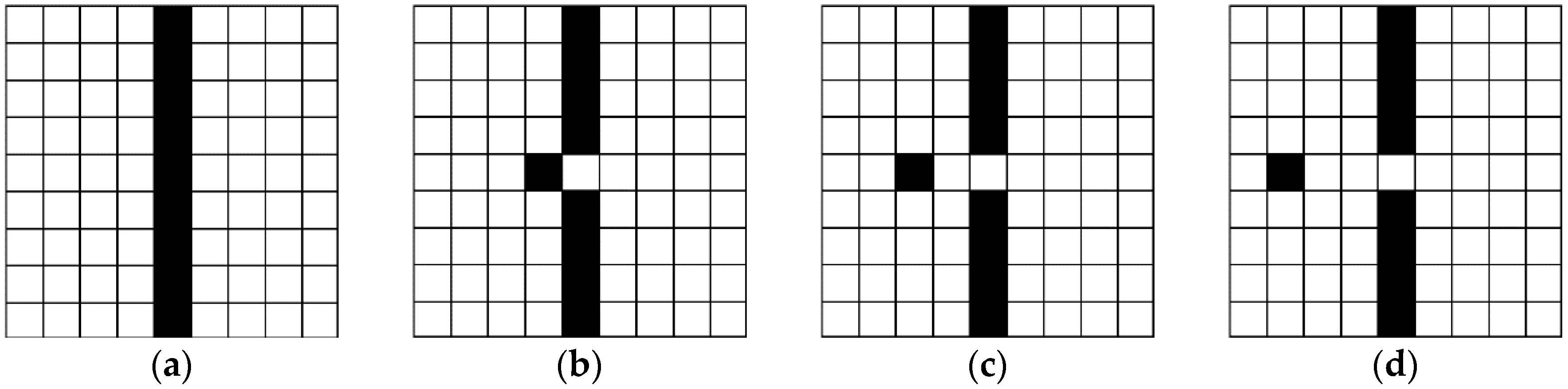
The Chi-square measure (6) can reflect the similarity of two edge maps, and the bigger the value of the Chi-square measurement, the better. As Lopez-Molina et al. stated in [19], the Chi-square measurement can evaluate the errors caused by spurious responses (false positives, FPs) and missing edges (false negatives, FNs), but it cannot work on the localization error when the detected edges deviate from their true position. For example, a reference edge image and three polluted edge maps are given in Figure 1. Compared with the reference edge (Figure 1a), the Chi-square measurements of the three polluted edge maps are the same, yet their localization accuracies are different. In order to reflect the localization error in these edge maps, distance-based error measures should be introduced.

The Baddeley’s delta metric (BDM) is one of the most common distance-based measures [20]. It has been proven to be an ideal measure for the comparison of edge detection algorithms [19,21]. Let A and B be two edge maps with the same resolution $M\times N$, and $P=\{1,\dots ,M\}\times \{1,\dots ,N\}$ be the set of pixels in the image. The value of BDM between A and B is defined as

$${\Delta }_{}^k(A,B)={\left[\frac{1}{MN}{\displaystyle \sum _{p\in P}{\left|w(d(p,A))-w(d(p,B))\right|}^k}\right]}^{1/k},$$

(7)

where $d(p,A)$ is the Euclidean distance from $p\in P$ to the closest edge points in A, the parameter $k$ is a given positive integer and $w(d(p,A))=\min (d(p,A),c)$ for a given constant $c>0$. Compared with the reference edge $E_R$ in Figure 1, the BDMs of the three polluted edge maps $E_i(i=1,2,3)$ are given in

Table 1. The Baddeley’s delta metrics (BDMs) between the reference edge image $E_R$ and the polluted edge maps $E_i(i=1,2,3)$ with the different choices of parameters c and k.

Parameter Sets	${\mathbf{\Delta }}^{\mathit{k}}({\mathit{E}}_{\mathit{R}},{\mathit{E}}_1)$	${\mathbf{\Delta }}^{\mathit{k}}({\mathit{E}}_{\mathit{R}},{\mathit{E}}_2)$	${\mathbf{\Delta }}^{\mathit{k}}({\mathit{E}}_{\mathit{R}},{\mathit{E}}_3)$
k = 1, c = 2	0.0566	0.0937	0.1256
k = 1, c = 3	0.0950	0.1879	0.2461
k = 1, c = 4	0.1397	0.2614	0.3305
k = 2, c = 2	0.2182	0.3307	0.3637
k = 2, c = 3	0.2753	0.4925	0.6313
k = 2, c = 4	0.3317	0.6159	0.8021

with different parameters $c$ and $k$. The smaller the value of BDM, the better. As we can see from Table 1, localization errors of the three edge maps are apparently distinguished. Therefore, the Chi-square measure (6) will be replaced by the BDM (7) in the choice strategies of the regularization parameter.

4. Experiments and Results

In order to show the validity of the proposed edge detection algorithm, some comparative experiments are given in this section. In the experiments, our regularized edge detector (RED) will be compared with the LoG detector and the Laplacian-based edge detector (LED) proposed in [7].

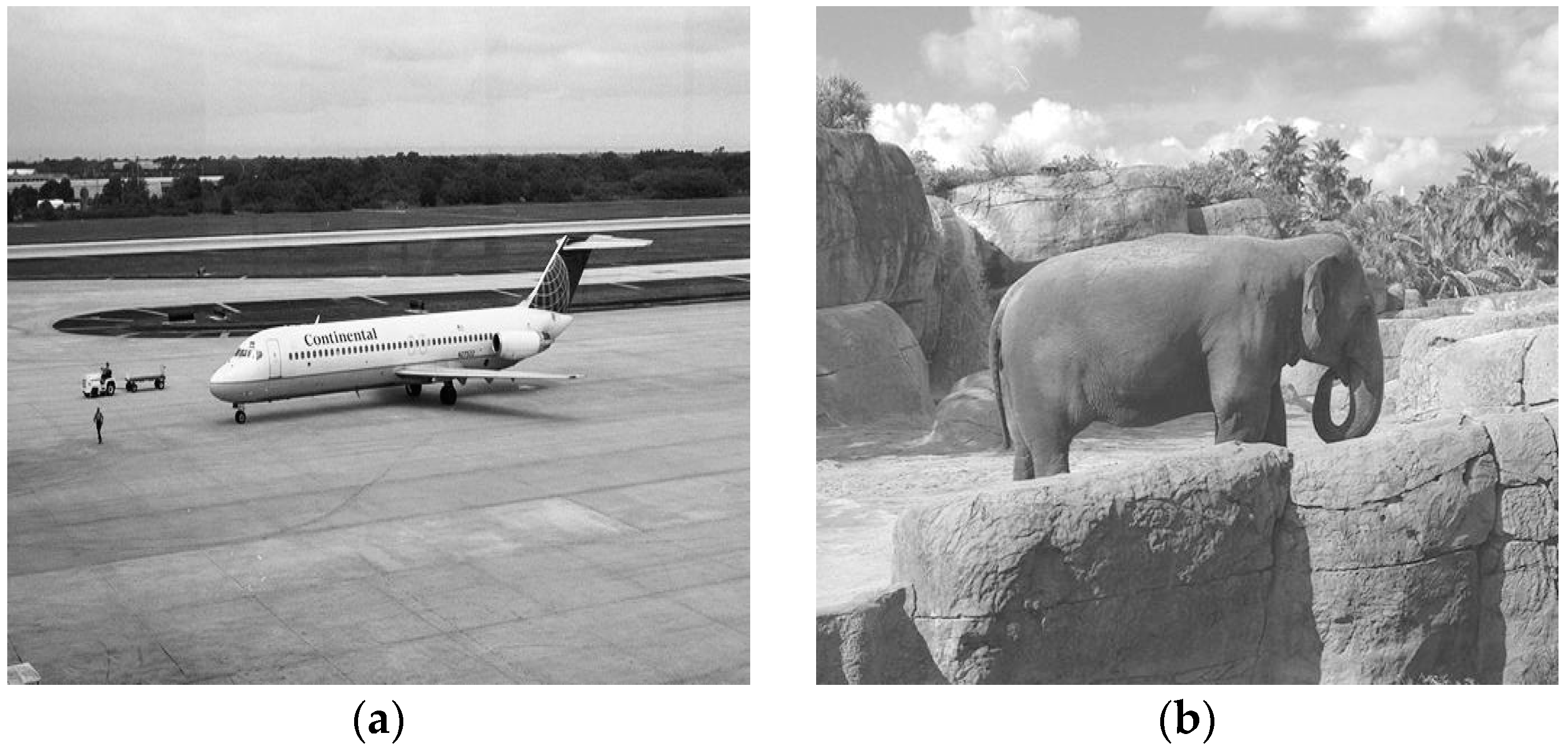
As Yitzhaky and Peli said in [17], the parameter selection for edge detection depends mainly on the set of parameters used to generate the initial detection results. In order to reduce this influence properly, the range of the parameter is set to be large enough that instead of forming a very sparse edge map it forms a very dense one. The scale parameter of the LoG detector is set from 1.5 to 4 in steps of 0.25. The regularization parameter of the regularized edge detector is set from 0.01 (≈0) to 0.1 in steps of 0.01. The images we used are taken from [22], and some of them are shown in Figure 2. The optimal edge maps given in [22] will be seen as the ground truth in our quantitative comparisons.

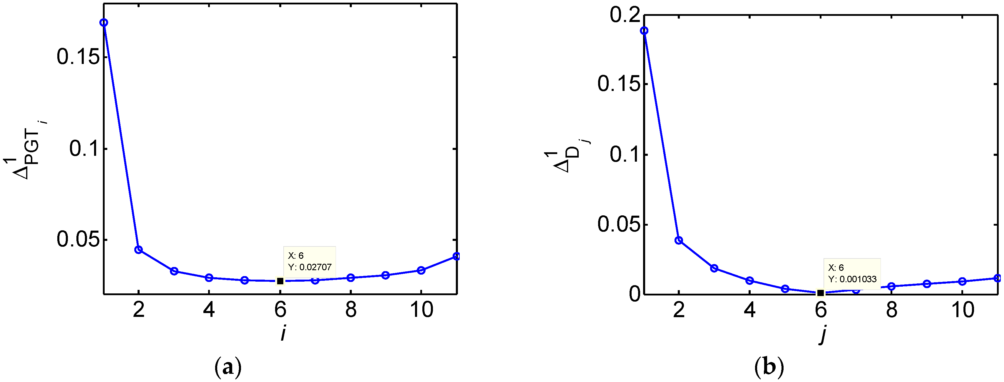
Let us first consider the choice strategy of the regularization parameter $\alpha$, where the parameters in BDM are set as $k=1,c=2$. Taking the airplane image as an example, the BDM of each ${\mathrm{PGT}}_i,i\in \{1,2,\dots 11\}$ is shown in Figure 3a, from which we can see the EGT is PGT₆. Compared with the EGT, the BDM of each edge map D_j is shown in Figure 3b, from which we can see the best edge map is D₆. Hence, the regularization parameter is chosen as $\alpha =0.05$. The choice of the scale parameter in the LoG detector is carried out similarly. It does not need any parameters in the LED.

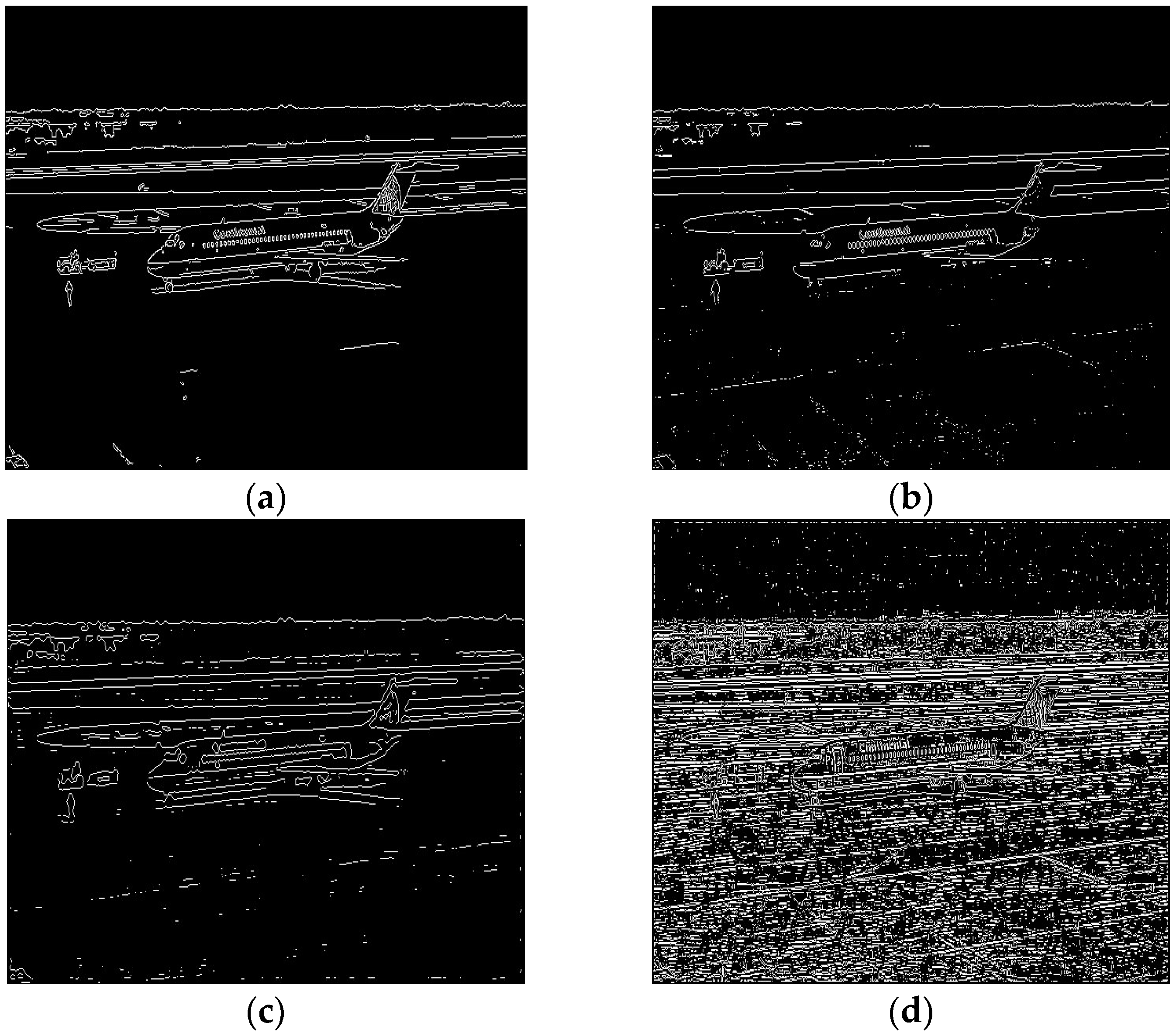
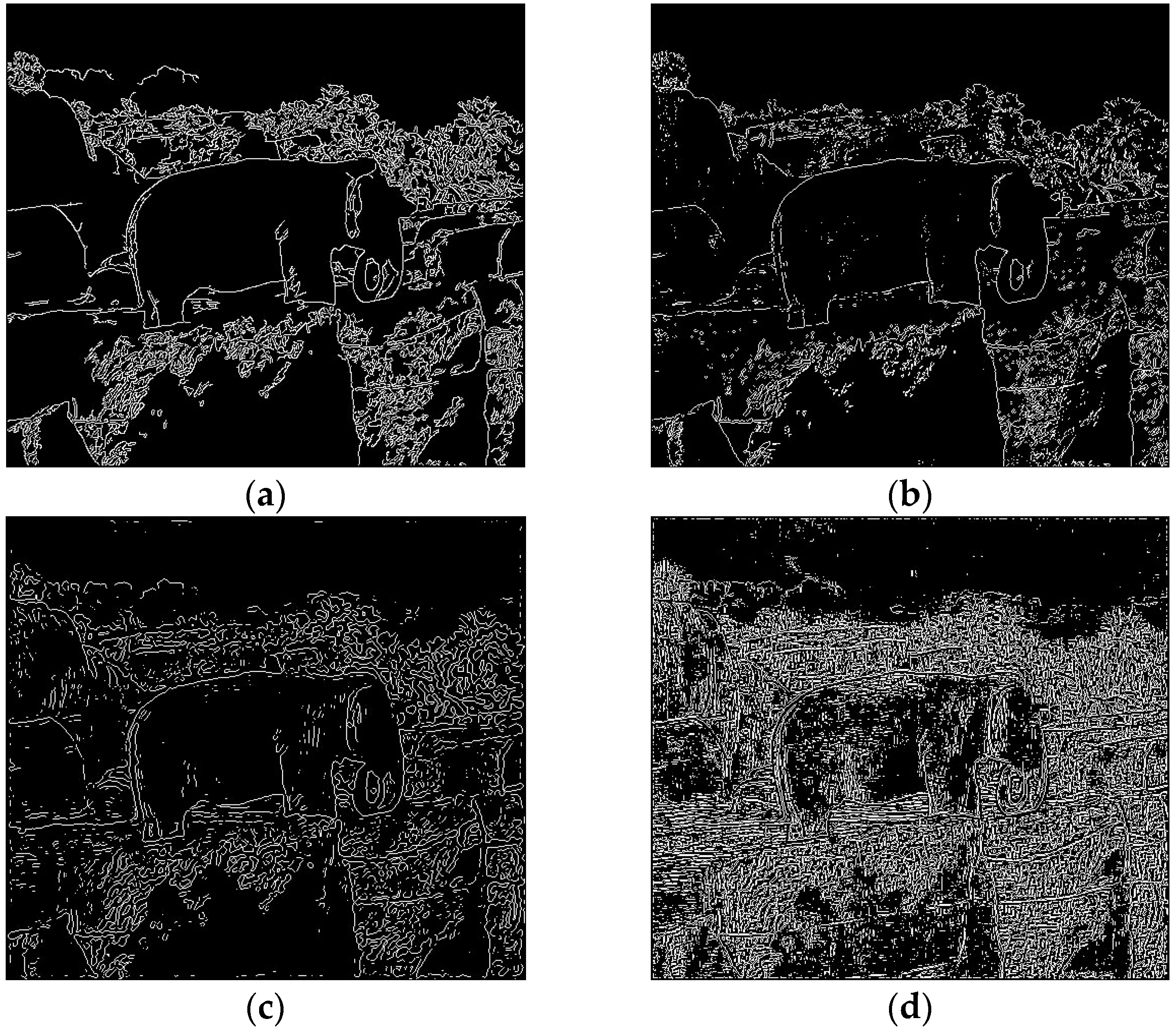
For the airplane image, the ground truth and edges detected by the three edge detectors are shown in Figure 4. From Figure 4b, we can see that the influence of the Lavrentiev regularization’s weakness on the RED is negligible. From Figure 4b,c, we can see that the RED is better than the LoG detector for noise suppression and maintaining continuous edges. Comparing Figure 4d with Figure 4b,c, we can see the superiority of the parameter-dependent edge detector. Similar results for the elephant image are shown in Figure 5. For some images taken from [22], quantitative comparisons of the edges detected by the LoG detector, the RED and the LED against the ground truth are given in

Table 2. Quantitative comparison of the edges detected by the LoG, the RED and the LED.

Images	LED	LoG	RED
Airplane	0.7515	0.1270	0.1232
Elephant	0.6619	0.3041	0.2593
Turtle	0.4430	0.1226	0.1323
Brush	0.5790	0.1883	0.1673
Tiger	0.9239	0.2854	0.2748
Grater	0.5537	0.2353	0.2143
Pitcher	0.5032	0.2584	0.2296

. Since the smaller the value of BDM, the better, this shows that the RED has better performance than the LoG detector and the LED in most cases.

5. Conclusions

In this paper, a novel edge detection algorithm is proposed based on the regularized Laplacian operation. The PDE-based regularization enables us to compute the regularized Laplacian operation in a direct way. Considering the importance of the regularization parameter, an objective choice strategy of the regularization parameter is proposed. Numerical implementations of the regularization parameter and the edge detection algorithm are also given. Based on the image database and ground truth edges taken from [22], the superiority of the RED against the LED and the LoG detector has been shown by the edge images and quantitative comparison.

References

- Basu, M. Gaussian-based edge-detection methods—A survey. IEEE Trans. Syst. Man Cybern. Part C Appl. Rev. 2002, 32, 252–260. [Google Scholar] [CrossRef]
- Marr, D.; Hildreth, E. Theory of edge detection. Proc. R. Soc. Lond. B 1980, 207, 187–217. [Google Scholar] [CrossRef] [PubMed] [Green Version]
- Canny, J. A computational approach to edge detection. IEEE Trans. Pattern Anal. Mach. Intell. 1986, 8, 679–698. [Google Scholar] [CrossRef] [PubMed]
- Sarkar, S.; Boyer, K. Optimal infinite impulse response zero crossing based edge detectors. CVGIP Image Underst. 1991, 54, 224–243. [Google Scholar] [CrossRef]
- Demigny, D. On optimal linear filtering for edge detection. IEEE Trans. Image Process. 2002, 11, 728–737. [Google Scholar] [CrossRef] [PubMed]
- Kang, C.C.; Wang, W.J. A novel edge detection method based on the maximizing objective function. Pattern Recognit. 2007, 40, 609–618. [Google Scholar] [CrossRef]
- Wang, X. Laplacian operator-based edge detectors. IEEE Trans. Pattern Anal. Mach. Intell. 2007, 29, 886–890. [Google Scholar] [CrossRef] [PubMed]
- Lopez-Molina, C.; Bustince, H.; Fernandez, J.; Couto, P.; De Baets, B. A gravitational approach to edge detection based on triangular norms. Pattern Recognit. 2010, 43, 3730–3741. [Google Scholar] [CrossRef]
- Murio, D.A. The Mollification Method and the Numerical Solution of Ill-Posed Problems; Wiley-Interscience: New York, NY, USA, 1993; pp. 1–5. ISBN 0-471-59408-3. [Google Scholar]
- Wan, X.Q.; Wang, Y.B.; Yamamoto, M. Detection of irregular points by regularization in numerical differentiation and application to edge detection. Inverse Probl. 2006, 22, 1089–1103. [Google Scholar] [CrossRef] [Green Version]
- Xu, H.L.; Liu, J.J. Stable numerical differentiation for the second order derivatives. Adv. Comput. Math. 2010, 33, 431–447. [Google Scholar] [CrossRef]
- Huang, X.; Wu, C.; Zhou, J. Numerical differentiation by integration. Math. Comput. 2013, 83, 789–807. [Google Scholar] [CrossRef]
- Wang, Y.C.; Liu, J.J. On the edge detection of an image by numerical differentiations for gray function. Math. Methods Appl. Sci. 2018, 41, 2466–2479. [Google Scholar] [CrossRef]
- Gonzalez, R.C.; Woods, R.E. Digital Image Processing, 3rd ed.; Pearson: London, UK, 2007; pp. 158–162. ISBN 978-0-13-168728-8. [Google Scholar]
- Gunn, S.R. On the discrete representation of the Laplacian of Gaussian. Pattern Recognit. 1999, 32, 1463–1472. [Google Scholar] [CrossRef]
- Xu, H.L.; Liu, J.J. On the Laplacian operation with applications in magnetic resonance electrical impedance imaging. Inverse Probl. Sci. Eng. 2013, 21, 251–268. [Google Scholar] [CrossRef]
- Yitzhaky, Y.; Peli, E. A method for objective edge detection evaluation and detector parameter selection. IEEE Trans. Pattern Anal. Mach. Intell. 2003, 25, 1027–1033. [Google Scholar] [CrossRef] [Green Version]
- Gu, C.H.; Li, D.Q.; Chen, S.X.; Zheng, S.M.; Tan, Y.J. Equations of Mathematical Physics, 2nd ed.; Higher Education Press: Beijing, China, 2002; pp. 80–86. ISBN 7-04-010701-5. (In Chinese) [Google Scholar]
- Lopez-Molina, C.; Baets De, B.; Bustince, H. Quantitative error measures for edge detection. Pattern Recognit. 2013, 46, 1125–1139. [Google Scholar] [CrossRef]
- Baddeley, A.J. An error metric for binary images. In Proceedings of the IEEE Workshop on Robust Computer Vision, Bonn, Germany, 9–11 March 1992; Wichmann Verlag: Karlsruhe, Germany, 1992; pp. 59–78. [Google Scholar]
- Fernández-García, N.L.; Medina-Carnicer, R.; Carmona-Poyato, A.; Madrid-Cuevas, F.J.; Prieto-Villegas, M. Characterization of empirical discrepancy evaluation measures. Pattern Recognit. Lett. 2004, 25, 35–47. [Google Scholar] [CrossRef]
- Heath, M.D.; Sarkar, S.; Sanocki, T.A.; Bowyer, K.W. A robust visual method for assessing the relative performance of edge detection algorithms. IEEE Trans. Pattern Anal. Mach. Intell. 1997, 19, 1338–1359. [Google Scholar] [CrossRef]
Figure 1.
The reference edge image and three polluted edge maps: (a) reference edge ; (b) polluted edge map ; (c) polluted edge map ; (d) polluted edge map .
Figure 2.
Some images taken from [22]: (a) airplane; (b) elephant.
Figure 3.
The figure of BDMs: (a) the BDM of ; (b) the BDM of .
Figure 4.
Edge detection results of the airplane image: (a) the ground truth; (b) the edge detected by the regularized edge detector (RED); (c) the Laplacian of Gaussian (LoG); (d) the Laplacian-based edge detector (LED).
Figure 5.
Edge detection results of the elephant image: (a) the ground truth; (b) the edge detected by the RED; (c) the LoG; (d) the LED.