Nonlocal Symmetries for Time-Dependent Order Differential Equations

Abstract

A new type of ordinary differential equation is introduced and discussed: time-dependent order ordinary differential equations. These equations are solved via fractional calculus by transforming them into Volterra integral equations of second kind with singular integrable kernel. The solutions of the time-dependent order differential equation represent deformations of the solutions of the classical (integer order) differential equations, mapping them into one-another as limiting cases. This equation can also move, remove or generate singularities without involving variable coefficients. An interesting symmetry of the solution in relation to the Riemann zeta function and Harmonic numbers is observed.

1. Introduction

It is rather the exception than the rule when large space-time scale complex systems, with their self-organization properties and competition–cooperation cycles, can be modeled with traditional, even nonlinear or stochastic, partial differential equations. The differential approach in modeling, very successful otherwise over a range of hundreds of years of science, is tributary to two strict features: dependence on given initial conditions, and evolution in a constant dimensional phase space. In the real world, however, the range of interaction between neighbor sub-systems, and the amount of memory relevant for different phases of evolution, are in continuous change [1,2]. In any brute force numerical simulation, the ranges of interaction and the memory length, or the history dependence, are controlled by the number of neighbors or time steps considered. In the continuous limit, these numbers determine the maximal orders of space and time derivatives in the continuous, differential model. The order of differentiation in a mathematical model determines the geometric structure of the differential equations, and the global structure of the solutions [3]. Thus, it is reasonable to assume that the changing of the type of behavior of a complex system [4,5] can be related, among other things, to the variation of the order of derivatives in the mathematical model [6]. One needs to introduce a new type of derivative and corresponding differential equation with time dependent order of differentiation, which can be generically expressed in the form

$$\frac{d^{\alpha \left(t\right)}}{d{t}^{\alpha \left(t\right)}}Y(t,x)=L\left[Y\right],$$

(1)

where $\alpha \left(t\right)$ is real function taking integer values at the ends of the domain of definition of t, Y is a function dependent on time t, and other independent (space) coordinates x, and L is a differential operator in the x variables. The punctuated equilibrium in evolution of living systems [7] or in the evolution of economy in some countries [8], and the wide variability of time scales in transient population growth rates, [9,10], memory dependent diffusion [11], networks with higher-order Markovian processes [12], and self-replicating clusters [13] are examples of systems whose dynamics change in time, and cannot be described by traditional differential approaches. For such systems, one needs new mathematical approaches by considering time-dependent order of differentiation with respect to space or time. This variable order changes in time from an integer order to another integer order, as limiting cases. In present population dynamics models, for example, authors use piece-wise defined differential equations artificially predicting transition from exponential behavior to singular hyperbolic behavior [14,15,16]. Another typical example where the order of the leading derivative must change during the evolution of the system is given by the drag force upon an accelerated submerged object. The dynamics change from inertia-less creep flow with force proportional to the first order time derivative (velocity), to Rayleigh drag with force proportional to the second order derivative (acceleration). One of the most promising applications of time dependent order differential/integral equations is the area of automatic control. This new type of dynamical changing equation could introduce a new class of fractional order proportional integral derivative controllers with higher achievable performances [17].

In the time-dependent order of differentiation, the system can change its dynamics during its evolution. This approach has a great advantage over the traditional modeling approach of using artificial time-dependent coefficients management. The use of time variable coefficients has implications of existence and uniqueness of solutions. Moreover, critical behavior of complex systems is inherent to the system, and not controlled by, or uniquely dependent on the change of constants of material. Moreover, this time-dependent order of differentiation manifestly changes the dimension of the phase space of the system.

When the order of differentiation changes continuously with time, it takes non-integer values. The correct formalism to handle such non-integer operators is provided by fractional calculus and fractional derivatives [18,19,20,21]. In this formalism, introduced since Riemann and Liouville and developed to a great extent in the last decades, the order of differentiation is a real constant. In the following, we rely in our calculations on this concept of fractional derivative.

This recent trend of time-variable order differential equations [6,22,23] is a possible candidate for modeling complex systems with complex unpredictable behavior. Time-dependent order of differentiation models can provide more realistic models for population growth in variable environments [10], fractional derivatives model for the general laws of predator-prey biological population dynamics [15], memory dependent diffusion [11], stochastic processes and multiplex networks described by higher-order Markovian processes [12], and boundary area and speed of action in self-replicating clusters [13]. Several authors reach toward the same target of developing time-dependent or space-dependent orders of differentiation, but starting from the different direction of trying to generalize fractional differential equations, and/or to model the dynamics of systems with variable constants of material [24,25,26,27,28,29,30].

In our previous studies [6,22,23], and in the present paper, we underline the benefits of introduction of time-dependent order of differentiation from the fundamental physical necessity of explaining complex systems. This field of research (also known under the name VODE or DODE as in variable/dynamical order differential equations) is still in its infancy, and a lot of caution should be considered in all hypotheses and conclusions. In the present paper, we analyze a simple model to understand better the properties of the time-dependent order differential equation, its solutions and their symmetries. Namely, we investigate a one-dimensional linear differential equations, with respect to time, whose order of differentiation changes in time with one unit.

The paper is organized as follows: following the Introduction, we present in Section 2 the time-dependent order differential equation and its properties and we briefly elaborate on the existence and uniqueness of the solutions. We also provide two examples when solutions are mapped through the variable order $\alpha \left(t\right)$ between two limiting cases represented by meromorphic functions with different positions of their singularities. In Section 3, we analyze Frobenius types of series solution for this new equation, and we present an interesting quasi-periodic symmetry. The paper is closed with Conclusions.

2. Time-Dependent Ordinary Differential Equation

In this section, we introduce a time-dependent one-dimensional differential equation for the function $x\left(t\right):(0,1)\to \mathbf{R}$ in the form

$$\frac{d^{\alpha \left(t\right)}x}{d{t}^{\alpha \left(t\right)}}=D^{\alpha \left(t\right)}x=f(t,x),$$

(2)

where $D^{\alpha }$ is the standard notation for fractional derivatives (to be defined below), the real function $\alpha \left(t\right)$ describes the time dependent order of differentiation, and f is the source term. As mentioned above, we represent the variable order through the formalism of fractional derivatives [18,19,20,21,31,32,33,34,35,36,37,38].

The fractional generalization of differential calculus can be defined in several types of fractional derivatives. For example, we can enumerate the fractional derivatives in the sense of Riemann-Liouville, Caputo, Grünwald, Jumarie, or Weyl [32,39]. These derivatives are non-local, and are able to model multiple scales systems, fractal differentiability, or nowhere differentiable functions [39]. The fractional derivatives and fractional integrals have applications in viscoelasticity, feedback amplifiers, electrical circuits, electro-analytical chemistry, fractional multipoles, neuron modeling and related areas in physics, chemistry, and biological sciences [20,33].

In the following, we use the Riemann–Liouville form of fractional derivative to introduce the time-dependent derivative

$${}_{t_0}{D}_t^{\alpha \left(t\right)}x\left(t\right)=\frac{d^m}{d{t}^m}\left(\frac{1}{\Gamma (m-\alpha (t\left)\right)}\underset{t_0}{\overset{t}{\int }}\frac{x\left(s\right)}{{(t-s)}^{\alpha \left(t\right)-m+1}}ds\right),$$

(3)

where the order $\alpha \left(t\right):{\mathbf{R}}_{+}\to [m-1,m)$, and $x\left(t\right):(0,1)\to \mathbf{R}$ are functions of class $C^m$, and m is a positive integer. In the following, we choose $t_0=0$, without any loss of generality [34,35], so we can skip the subscripts from the expression of the fractional derivative. This derivative operator does not obey the standard Leibnitz rule [18,19]. It is actually proved (Equation (3.39) in [18]) that the fractional generalization of the Leibniz rule for such Riemann–Liouville operators is expressed in terms of infinite series. The fractional derivative converges uniformly towards the integer value at its bounds ${lim}_{\alpha \left(t\right)->{(m-1)}^{+}}{D}^{\alpha \left(t\right)}x\left(t\right)=x^{(m-1)}$, and ${lim}_{\alpha \left(t\right)->m^{-}}{D}^{\alpha \left(t\right)}x\left(t\right)=x^{\left(m\right)}$ [23].

We consider two initial value problems for a time-dependent ordinary differential equation. In the first case, we ch0ose $\alpha \left(t\right)\in [0,1]$, that is $m=1$ in Equation (3), and the differential equations has the form

$$D^{\alpha \left(t\right)}(x-x_0)=f(t,x\left(t\right)),x\left(0\right)=x_0,$$

(4)

where $t\in (0,1),x_0\in \mathbf{R}$, the order of differentiation function is a continuous function $\alpha :(0,1)\to [0,1]$, and the source term is a continuous function $f:{\mathbf{R}}_{+}\times \mathbf{R}\to \mathbf{R}$.

In the second case, we choose $\alpha \left(t\right)\in [1,2]$, that is $m=2$ in Equation (3), and we have the form

$$D^{\alpha \left(t\right)}(y-y_0-y_{1}t)=g(t,y\left(t\right)),y\left(0\right)=y_0,y^{\prime }\left(0\right)=y_1,$$

(5)

where $t\in (0,1),y_0,y_1\in \mathbf{R}$, the order of differentiation function is a continuous function $\alpha :(0,1)\to [1,2]$, and the source term is a continuous function $g:{\mathbf{R}}_{+}\times \mathbf{R}\to \mathbf{R}$.

The way the initial data problem is formulated, even in the time-independent fractional differential equations case, is still in debate, and its physical meaning is not yet fully understood [18,37]. Therefore, the incorporation of classical derivatives of the initial data in Equation (4) was suggested by many authors [11,35,37], as they are commonly used in initial value problems with integer-order equations.

It is proved [6,22] that the initial value problem in Equations (4) and (5) are reducible to Volterra integral equations of the second kind with singular integrable kernel. In the case of Equation (4), we have $k(t,\tau )={(t-\tau )}^{\alpha \left(t\right)-1}$, as long as $\alpha \left(t\right)\in (0,1)$

$$x\left(t\right)=x_0+\frac{1}{\Gamma \left(\alpha \right(t\left)\right)}\underset{0}{\overset{t}{\int }}\frac{f(\tau ,x(\tau \left)\right)d\tau }{{(t-\tau )}^{1-\alpha \left(t\right)}}.$$

(6)

In a similar way, Equation (5) can be mapped into a similar Volterra integral equation of the second kind with singular integrable kernel

$$y\left(t\right)=y_0+t{y}_1+\frac{1}{\Gamma \left(\alpha \right(t)-1)}{\int }_{t_0}^t\frac{{\int }_{t_0}^{\tau }g(s,y\left(s\right))ds}{{(t-\tau )}^{2-\alpha \left(t\right)}}d\tau .$$

(7)

Any solution of Equations (6) and (7) is a solution of the initial value problem in Equations (4) and (5), respectively. The solutions for Equations (6) and (7) smoothly approach the classical solutions of the corresponding classical differential equations of integer order in the limiting integer values of $\alpha =0,1,2$. 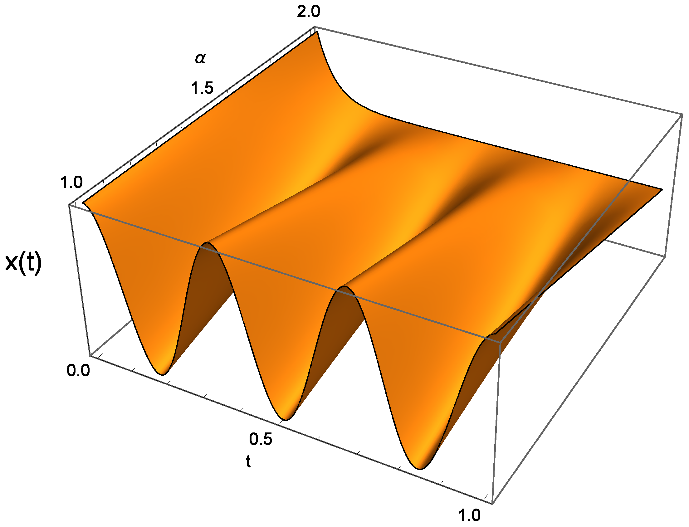For the cases when the solutions are smooth and regular all over their domain of definition, the conditions of existence and uniqueness of smooth solutions of Equations (6) and (7) are covered in [6,23]. non-ho In Figure 1, we present an example of smooth solution for Equation (5) with $\alpha \in (1,2)$, for a non-homogeneous term of the form $g(t,y)=-y$ and $y_0=1,y_1=-1$. The solution was obtained numerically for the integral version (Equation (7)) of Equation (5). In the limiting cases of integer order of differentiation, it is easy to verify that the limiting solutions are

$$y\left(t\right)=\left\{\begin{array}{c}{e}^{-t}\mathrm{for}\alpha =1,\hfill \\ cost\mathrm{for}\alpha =2,\hfill \end{array}\right.$$

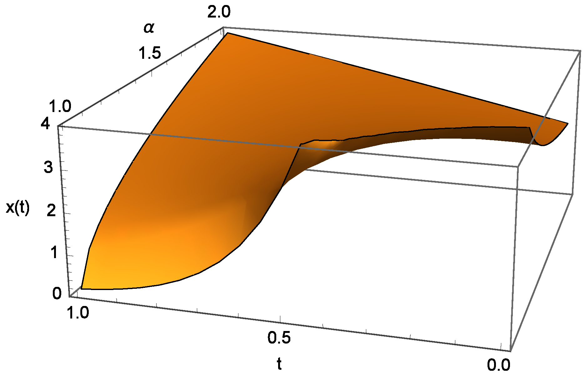
One can notice in Figure 1 how the solution smoothly maps from negative exponential to periodic trigonometric function, with the change of the order of differentiation in the differential equation. More interesting situations occur in the case when the solutions have singularities. In this case, we cannot apply the existence and uniqueness from [6,23], and a different approach is developed in the following. We present such a transition from a smooth to a singular solution in Figure 2, and Equation (8). This is again an example of solution for Equation (5) with $\alpha \in (1,2)$, but for a non-homogeneous term of the form $g(t,y)=-t^{-3/2}$. The solution was obtained numerically for the integral version (Equation (7)) of Equation (5). In the limiting cases of integer order of differentiation, it is easy to verify that the limiting solutions are

$$y\left(t\right)=\left\{\begin{array}{c}\frac{2}{\sqrt{t}}+C_0,\mathrm{for}\alpha =1,\hfill \\ 4\sqrt{t}+C_0+C_{1}t,\mathrm{for}\alpha =2,\hfill \end{array}\right.$$

(8)

where specifically in the case of Figure 2 we have $C_0=0,C_1=1$. The numerical solution of the time-dependent order differential equation smoothly connects these two limiting cases, and makes a smooth transition from a solution with singularity at $t=0$ for $\alpha =1$ to a smooth solution on $t\in (0,1)$ for $\alpha =2$.

3. Initial Value Problem and Non-Local Symmetries

To analyze the well-posedness of the initial value problem for time-variable order differential equations of the type in Equations (4) and (5) or equivalently the integral non-local forms in Equations (6) and (7), we present here a particular case when $f(t,x(t\left)\right)=x\left(t\right)$. In the general case for the non-homogeneous term f, one can use the same procedures, except the calculations become too long and tedious to be presented here. The first observation is that one cannot use traditional expansions of the hypothetical solution $x\left(t\right)$ or $y\left(t\right)$, respectively, in Frobenius series because the series coefficients turn to be time variable, a fact which contradicts the hypothesis. Indeed, by considering the transition $\alpha :0\to 1$ for $x\left(t\right)$ for Equation (6), and using a power series solution in the form

$${\displaystyle x\left(t\right)=x_0+t^r\sum _{j=0}^{\infty }{c}_j{t}^j,}$$

(9)

with constant coefficients, when we plug the series in Equation (9) into Equation (6), we obtain

$$x\left(t\right)=x_0+\frac{x_0{t}^{\alpha \left(t\right)}}{\alpha \left(t\right)\Gamma \left(\alpha \right(t\left)\right)}$$

$${\displaystyle +\frac{t^{r+\alpha \left(t\right)}}{\Gamma (r+\alpha (t\left)\right)}\sum _{k=1}^{\infty }\frac{t^k(k+r)c_k\Gamma (k+r)}{{\displaystyle \prod _{j=0}^k(r+j+\alpha \left(t\right))}}.}$$

(10)

Consequently, the series in Equation (9) is forced to have time-dependent coefficients, which contradicts the hypothesis on the one hand, and does not necessarily guarantee convergence, on the other hand. Moreover, even in the simplest linear form for the time-dependent order $\alpha \left(t\right)=t$, the first orders in powers of t in Equation (10) provide a singular logarithmic time dependence around zero for the series coefficients, for example

$$x\left(t\right)=x_0+t^r[t{c}_1+t^2(c_2+c_{1}lnt-c_1\psi (2+r))]+t^r{\mathcal{O}}_3,$$

(11)

where $\psi$ is the digamma function. By comparison with Equation (9), it is obvious that even in the simplest linear case for the time-dependence of the order of differentiation, the solution $x\left(t\right)$ is not holomorphic and has logarithmic singularity at $x=0$, therefore one needs to use a different procedure.

Consequently, we expand the hypothetical solution $x\left(t\right)$ in a Taylor series, and then use a similar procedure as in [23]. In the following, we assume that the solution is an analytic function on $(0,1)$, $x\left(t\right)\in C^{\infty }(0,1)$, and its Taylor series around $t\in (0,1)$

$$x\left(\tau \right)=\sum _{n\ge 0}\frac{{(\tau -t)}^n{x}^{\left(n\right)}\left(t\right)}{n!},$$

(12)

converges absolutely and uniformly as a functional series in variable $\tau \in (0,1)$. We also assume that this solution has the property that its integral from the right hand side term of Equation (6) converges absolutely. We introduce the Taylor series given by Equation (12) into Equation (6) and we obtain

$$x\left(t\right)-x_0=\frac{1}{\Gamma \left(\alpha \right(t\left)\right)}{\int }_0^t\sum _{n\ge 0}\frac{{(\tau -t)}^n{x}^{\left(n\right)}\left(t\right)}{n!}{(t-\tau )}^{\alpha \left(t\right)-1}d\tau .$$

Since the solution $x\left(t\right)$ is chosen to be analytic and represented by an absolutely and uniformly convergent Taylor series for any $t,\tau \in (0,1)$, and the above integrals are absolutely convergent for any term of the Taylor series, and for the sum of the Taylor series, it results that the integral commutes with the series. By interchanging the order between the integral and the series, and by integrating term by term with respect to $\tau$, we have

$$x\left(t\right)-x_0=\frac{1}{\Gamma \left(\alpha \right(t\left)\right)}\sum _{n\ge 0}\frac{{(-1)}^n{x}^{\left(n\right)}\left(t\right)}{n!}\left(-\frac{t^{\alpha \left(t\right)+n}}{\alpha \left(t\right)+n}\right)(-1),$$

all the other terms being zero when we evaluate the limits of integration at $\tau -t$. Consequently, we can write

$$x_0+\left(\frac{t^{\alpha \left(t\right)}}{\Gamma \left(\alpha \right(t)+1)}-1\right)x\left(t\right)+\frac{t^{\alpha \left(t\right)}}{\Gamma \left(\alpha \right(t\left)\right)}\sum _{n\ge 1}\frac{{(-1)}^n{t}^n}{\left(\alpha \right(t)+n)n!}{x}^{\left(n\right)}\left(t\right)=0,$$

(13)

where we separated the term with $n=0$ from the other terms in the series, and where $x^{\left(n\right)}\left(t\right)=d^{n}x/d{t}^n$ and $\alpha \in (0,1)$. The functional series in Equation (13) is convergent because it is bounded from above by the convergent series

$$x_0=\sum _{n\ge 0}\frac{{(-1)}^n{t}^n}{n!}{x}^{\left(n\right)}\left(t\right)=0,$$

and it has the radius of convergence given by some neighborhood of $t=0$ including $(0,1)$. We mention that the functional series in Equation (13) is not a Taylor or Frobenius series, or an expansion of some function in a complete or not system of functions. It is just an expression for which we know it is convergent given the precautions we took within this paragraph for the function $x\left(t\right)$.

Actually, Equation (13) can be regarded as an infinite order linear ordinary differential equation with time-dependent continuous coefficients for $x\left(t\right)$. That is an ordinary differential equation of infinite order whose coefficients are time-dependent functions. In other words, Equation (13) can be written in the form

$$x_0+a_0\left(t\right)x\left(t\right)+a_1\left(t\right)x^{\prime }\left(t\right)+a_2\left(t\right)x^{″}\left(t\right)+\cdots =0.$$

All the coefficients $a_n\left(t\right)$ are non-singular at $t=0$ independent of the value of $\alpha \left(0\right)$. The Koch–Lalescu–Gramegna theorem (see Equation (29) in [40]) states that such infinite systems have unique analytic solution on a neighborhood of $t=0$ where all coefficients $a_n\left(t\right)$ are analytic, providing the infinite set of initial conditions is given $x\left(0\right)=x_0,x^{\prime }\left(0\right)=x_1,x^{″}\left(0\right)=x_2,\cdots$.

If we expand again $x\left(t\right)$ in Taylor series, this time around $t=0$, and plug the series into Equation (6), we obtain

$$x\left(t\right)=x_0+t^{\alpha \left(t\right)}\sum _{n\ge 0}\frac{t^n{x}^{\left(n\right)}\left(0\right)}{\Gamma \left(\alpha \right(t)+n+1)},$$

from where it is straightforward to note that the whole infinite series of initial conditions $x^{\prime }\left(0\right),x^{″}\left(0\right),\cdots$ can be obtained algebraically only from $x\left(0\right)$ and $\alpha \left(t\right)$. This final result proves that the problem in Equation (2) for $f=x\left(t\right)$, and consequently the problem in Equation (6) for the same f are well posed for one initial condition $x\left(0\right)=x_0$, as long as we maintain t in the analyticity neighborhood mentioned above and also if ${lim}_{t\to 0}{t}^{\alpha \left(t\right)}$ is finite (which we know it is 0 or 1 if $\alpha \in (0,1)$. A similar treatment and a similar conclusion happen for $\alpha \in (1,2)$ and Equation (7), respectively, etc. The solutions $x\left(t\right)$ involve Riemann zeta function, as well as fractional harmonic numbers.

In the following, we present another interesting symmetry of the solutions of Equations (6) and (7) with respect to the variation of the order of differentiation. We present the following result: for m positive integer and for any continuous functions $\alpha \left(t\right):(0,1)\to (m-1,m)$, and $g\left(t\right):(0,1)\to \mathbf{R}$, there are always two distinct values ${\alpha }_1\ne {\alpha }_2$ in $(m-1,m)$ such that the equality

$${\displaystyle \frac{1}{\Gamma \left({\alpha }_1\right)}{\int }_0^{t}g\left(\tau \right){(t-\tau )}^{{\alpha }_1}d\tau =\frac{1}{\Gamma \left({\alpha }_2\right)}{\int }_0^{t}g\left(\tau \right){(t-\tau )}^{{\alpha }_2}d\tau ,}$$

(14)

where $g\left(t\right)=f(t,x(t\left)\right)$, is fulfilled for some $t\in (0,1)$. To prove this relation, we re-write Equation (14) in the form

$${\displaystyle \frac{1}{\Gamma \left({\alpha }_2\right)}{\int }_0^t\frac{f(\tau ,x(\tau \left)\right)}{{(t-\tau )}^{-{\alpha }_2}}\left(\frac{\Gamma \left({\alpha }_2\right)}{\Gamma \left({\alpha }_1\right){(t-\tau )}^{{\alpha }_2-{\alpha }_1}}-1\right)d\tau =0.}$$

Without any loss of generality, we assume ${\alpha }_2>{\alpha }_1$. The bottom limit $\tau \to 0^{+}$ of the integrand of the above integral is

$$\frac{f(0,x_0)}{t^{-{\alpha }_2}}\left(\frac{\Gamma \left({\alpha }_2\right)}{\Gamma \left({\alpha }_1\right)t^{{\alpha }_2-{\alpha }_1}}-1\right),$$

and can be always tuned to be an arbitrary large negative number. Indeed, by restricting $t\in (0,1)$, we have $t^{{\alpha }_2-{\alpha }_1}\in (0,1)$, and for any given ${\alpha }_2$ we can find ${\alpha }_1$ such that $\Gamma \left({\alpha }_2\right)<\Gamma \left({\alpha }_1\right)t^{{\alpha }_2-\alpha 1}$ since $\Gamma$ is local monotonic, and we can choose ${\alpha }_{1,2}$ in the region where $\Gamma$ is strictly decreasing. At the same time, we have

$${\displaystyle \underset{\tau \to t}{lim}\frac{f(\tau ,x(\tau \left)\right)}{{(t-\tau )}^{-{\alpha }_2}}\left(\frac{\Gamma \left({\alpha }_2\right)}{\Gamma \left({\alpha }_1\right){(t-\tau )}^{{\alpha }_2-{\alpha }_1}}-1\right)=+\infty .}$$

We obtain that the integrand oscillates between an arbitrary large negative value and plus infinity, while is guaranteed for the integral to be convergent by the theorem of existence of the solution [6]. It results that we can always find a value for ${\alpha }_1$ such that this integral is zero, and the affirmation in Equation (14) is proved.

4. Conclusions

In this paper, we introduce and discuss properties of time-dependent order ordinary differential equations. We show that such new types of differential equations can be represented in terms of generalizations of fractional derivatives with time-dependent order of differentiation. This approach allows us to map the time-dependent ordinary differential equation to a Volterra integral equation of second kind with singular integrable kernel, which is known to have a unique solution for appropriately chosen initial conditions and smoothness of the parameters and solution. We demonstrate that the general solution of this time-dependent order differential equations can smoothly deform the corresponding limiting solutions of the classical integer order ordinary differential equations, one into another, and can even generate singularities from regular solutions, and vice versa. We present a proof for the well posedness of the initial condition problem for such equations, and we also put into evidence interesting symmetry of the solution.