Numerical Simulation of PDEs by Local Meshless Differential Quadrature Collocation Method

Abstract

In this paper, a local meshless differential quadrature collocation method based on radial basis functions is proposed for the numerical simulation of one-dimensional Klein–Gordon, two-dimensional coupled Burgers’, and regularized long wave equations. Both local and global meshless collocation procedures are used for spatial discretization, which convert the mentioned partial differential equations into a system of ordinary differential equations. The obtained system has been solved by the forward Euler difference formula. An upwind technique is utilized in the case of the convection-dominated coupled Burgers’ model equation. Having no need for the mesh in the problem domain and being less sensitive to the variation of the shape parameter as compared to global meshless methods are the salient features of the local meshless method. Both rectangular and non-rectangular domains with uniform and scattered nodal points are considered. Accuracy, efficacy, and the ease of implementation of the proposed method are shown via test problems.

1. Introduction

The Klein–Gordon (KG) equation can describe various vital phenomena in chemical and physical sciences. The KG equation can be written as:

$$\frac{{\partial }^{2}U}{\partial t^2}+\alpha \frac{{\partial }^{2}U}{\partial x^2}+\beta U+\gamma U^2=h(x,t),x\in [a,b],t>0,$$

(1)

along with initial and boundary conditions:

$$\begin{array}{cc}\hfill U(x,0)& =h_1\left(x\right),\frac{\partial U(x,0)}{\partial t}=h_2\left(x\right),\hfill \\ \hfill U(a,t)& =h_3\left(t\right),U(b,t)=h_4\left(t\right),\hfill \end{array}$$

(2)

where $\alpha$, $\beta$, and $\gamma$ are the parameters.

The nonlinear KG equation has applications in numerous fields such as nonlinear optics, quantum mechanics, solid state physics, and in mathematical physics [1,2]. Various numerical techniques are employed for solving the KG equation such as the symplectic finite difference method [3], the spectral method [4], the meshless RBF method [5], the finite-difference collocation method [6], the differential quadrature method [7], the Haar wavelet method [8], the decomposition method [2], the Laplace transformation and Legendre wavelets method [9], the lattice Boltzmann method [10], and the multiquadric quasi-interpolation method [11].

The 2D coupled Burgers’ equations [12,13,14,15] can be written as:

$$\begin{array}{cc}\hfill \frac{\partial U}{\partial t}+U\frac{\partial U}{\partial x}+V\frac{\partial U}{\partial y}-\frac{1}{Re}\left(\frac{{\partial }^{2}U}{\partial x^2}+\frac{{\partial }^{2}U}{\partial y^2}\right)& =0,(x,y)\in \mathrm{\Omega }\hfill \\ \hfill \frac{\partial V}{\partial t}+U\frac{\partial V}{\partial x}+V\frac{\partial V}{\partial y}-\frac{1}{Re}\left(\frac{{\partial }^{2}V}{\partial x^2}+\frac{{\partial }^{2}V}{\partial y^2}\right)& =0,(x,y)\in \mathrm{\Omega }\hfill \end{array}$$

(3)

with initial and boundary conditions:

$$\begin{array}{cc}\hfill U(x,y,0)& =I_1(x,y),V(x,y,0)=I_2(x,y),(x,y)\in \mathrm{\Omega }\hfill \\ \hfill U(x,y,t)& =B_1(x,y,t),V(x,y,t)=B_2(x,y,t),(x,y)\in \partial \mathrm{\Omega }\hfill \end{array}$$

(4)

where $Re$ is a real constant known as the Reynolds number.

The coupled Burgers’ equations are related to many physical problems including traffic flow, acoustic transmission, flow of a shock wave traveling in a viscous fluid, airfoil flow theory, supersonic flow, and in turbulence phenomena (see [12,13,14,15] and the references therein for details).

The 2D nonlinear regularized long wave (RLW) equation with initial and boundary conditions can be written as [16,17],

$$\begin{array}{c}\hfill \frac{\partial U}{\partial t}-\frac{\partial }{\partial t}\left(\frac{{\partial }^{2}U}{\partial x^2}+\frac{{\partial }^{2}U}{\partial y^2}\right)+\frac{\partial U}{\partial x}+\frac{\partial U}{\partial y}+U\frac{\partial U}{\partial x}+U\frac{\partial U}{\partial y}=0,(x,y)\in \mathrm{\Omega },t>0,\end{array}$$

(5)

$$\begin{array}{cc}\hfill U(x,y,0)& =g_1(x,y),(x,y)\in \mathrm{\Omega }\hfill \\ \hfill U(x,y,t)& =g_2(x,y,t),U(x,y,t)=g_3(x,y,t).(x,y)\in \partial \mathrm{\Omega }\hfill \end{array}$$

(6)

The regularized long wave (RLW) model equation has described many physical phenomena [18]. So far, the existing literature contains many numerical methods used for solving the RLW equation such as finite-difference methods [19,20], the interpolating element-free Galerkin method [17], the finite-element method [21], the Fourier pseudo-spectral method [22], and the cubic B-spline method [23]. Furthermore, the Petrov–Galerkin method [24] and the element-free kp-Ritz method [25] are used for the generalized RLW equation.

Recently, meshless methods have seen broad attention for solving different kinds of PDE model areas in almost all disciplines of engineering. The meshless character is one of the most important reasons for the rising demand of such types of methods. Meshless methods reduce the complexity caused due to dimensionality to a large extent, which is faced in the carrying out of conventional methods like the finite-element and finite-difference procedures. Meshing in the case of complicated geometries is another cause for the growing demand of meshless methods. The numerical results of RBF-based algorithms have demonstrated that they are truly meshless, accurate, and easy to implement. Some interesting models can be found in [26,27,28,29,30].

It is noted that the global meshless method (GMM), which is based on the global interpolation paradigm, has faced the problems of dense ill-conditioned matrices and finding the optimum value of the shape parameter. To avoid the limitations of the GMM, a local meshless method, which is based on local interpolation in the sub-domains, is used as a substitute to get a stable and accurate solution for the PDE models (see [31,32,33,34,35,36,37]).

In the current work, the local meshless differential quadrature collocation method (LMM) based on radial basis functions (RBFs) is proposed for the numerical simulation of 1D nonlinear KG, 2D coupled Burgers’ equations, and the 2D RLW equation. The LMM is an accurate and efficient numerical technique, which requires two steps to approximate a time-dependent PDEs. Firstly, the spatial derivatives are approximated by using the RBFs, which could convert the given PDE into a system of ODEs. Then, the obtained ODEs will be solved by suitable ODE solvers.

The rest of the paper is organized as follows: the suggested numerical method is highlighted in Section 2; the implementation of the method with different test problems is presented in Section 3; and finally, some concluding remarks are given in Section 4.

2. Implementation of the Numerical Method

The LMM [26,33] is extended to the PDE models discussed in Section 1. The derivatives of $U(\mathbf{x},t)$ at the center ${\mathbf{x}}_i$ are approximated by the function values at a set of nodes in the neighborhood of $\{{\mathbf{x}}_{i1},{\mathbf{x}}_{i2},{\mathbf{x}}_{i3},\dots ,{\mathbf{x}}_{i{n}_i}\}\subset \{{\mathbf{x}}_1,{\mathbf{x}}_2,\dots ,{\mathbf{x}}_{N^n}\},n_i\ll N^n$, where $i=1,2,\dots ,N^n$. For the one-dimensional case, $n=1$ and $\mathbf{x}=x$, and for the two-dimensional case, $n=2$ and $\mathbf{x}=(x,y)$.

Now, for the 1D case, we have:

$$U^{\left(m\right)}\left(x_i\right)\approx \sum _{k=1}^{n_i}{\lambda }_k^{\left(m\right)}U\left(x_{ik}\right),i=1,2,\dots ,N.$$

(7)

To find the corresponding coefficient ${\lambda }_k^{\left(m\right)}$, radial basis function $\psi (\parallel x-x_l\parallel )$ can be substituted in Equation (7) as follows:

$${\psi }^{\left(m\right)}(\parallel x_i-x_l\parallel )=\sum _{k=1}^{n_i}{\lambda }_{ik}^{\left(m\right)}\psi (\parallel x_{ik}-x_l\parallel ),l=i1,i2,\dots ,i{n}_i,$$

(8)

where $\psi (\parallel x_{ik}-x_l\parallel )=\sqrt{1+(c\parallel x_{ik}-x_l{\parallel )}^2}$ and $\psi (\parallel x_{ik}-x_l\parallel )={\left(1+(c\parallel x_{ik}-x_l\parallel \right)}^2{)}^{-1}$ in the case of multiquadric (MQ) and inverse quadratic (IQ) radial basis functions, respectively.

The matrix notation of Equation (8) is:

$${\mathit{\psi }}_{n_i}^{\left(m\right)}={\mathbf{A}}_{n_i}{\mathit{\lambda }}_{n_i}^{\left(m\right)},$$

(9)

where:

$${\mathit{\psi }}_{n_i}^{\left(m\right)}={\left[\begin{array}{cccc}{\psi }_{i1}^{\left(m\right)}\left(x_i\right)& {\psi }_{i2}^{\left(m\right)}\left(x_i\right)& \cdots & {\psi }_{i{n}_i}^{\left(m\right)}\left(x_i\right)\end{array}\right]}^T,$$

$${\mathbf{A}}_{n_i}=\left[\begin{array}{cccc}{\psi }_{i1}\left(x_{i1}\right)& {\psi }_{i2}\left(x_{i1}\right)& \cdots & {\psi }_{i{n}_i}\left(x_{i1}\right)\\ {\psi }_{i1}\left(x_{i2}\right)& {\psi }_{i2}\left(x_{i2}\right)& \cdots & {\psi }_{i{n}_i}\left(x_{i2}\right)\\ ⋮& ⋮& \ddots & ⋮\\ {\psi }_{i1}\left(x_{i{n}_i}\right)& {\psi }_{i2}\left(x_{i{n}_i}\right)& \cdots & {\psi }_{i{n}_i}\left(x_{i{n}_i}\right)\end{array}\right],$$

$${\mathit{\lambda }}_{n_i}^{\left(m\right)}={\left[\begin{array}{cccc}{\lambda }_{i1}^{\left(m\right)}& {\lambda }_{i2}^{\left(m\right)}& \cdots & {\lambda }_{i{n}_i}^{\left(m\right)}\end{array}\right]}^T.$$

From Equation (9), we obtain:

$${\mathit{\lambda }}_{n_i}^{\left(m\right)}={\mathbf{A}}_{n_i}^{-1}{\mathit{\psi }}_{n_i}^{\left(m\right)}.$$

(10)

From Equations (7) and (10), we get:

$$\begin{array}{c}\hfill U^{\left(m\right)}\left(x_i\right)={\left({\mathit{\lambda }}_{n_i}^{\left(m\right)}\right)}^T{\mathbf{U}}_{n_i},\end{array}$$

where:

$${\mathbf{U}}_{n_i}={\left[U\left(x_{i1}\right),U\left(x_{i2}\right),\dots ,U\left(x_{i{n}_i}\right)\right]}^T.$$

For the 2D case, the derivatives of $U(x,y,t)$ with respect to x are approximated in a similar way as stated above and can be written as:

$$U_x^{\left(m\right)}(x_i,y_i)\approx \sum _{k=1}^{n_i}{\gamma }_k^{\left(m\right)}U(x_{ik},y_{ik}),i=1,2,\dots ,N^2,$$

(11)

and the corresponding coefficients ${\gamma }_k^{\left(m\right)},k=1,2,\dots ,n_i$ can be found as follows:

$${\mathit{\gamma }}_{n_i}^{\left(m\right)}={\mathbf{A}}_{n_i}^{-1}{\mathbf{\Phi }}_{n_i}^{\left(m\right)}.$$

(12)

Similarly, the derivatives of $U(x,y,t)$ with respect to y and its corresponding coefficients ${\eta }_k^{\left(m\right)},k=1,2,\dots ,n_i$ can be found as follows:

$$U_y^{\left(m\right)}(x_i,y_i)\approx \sum _{k=1}^{n_i}{\eta }_k^{\left(m\right)}U(x_{ik},y_{ik}),i=1,2,\dots ,N^2,$$

(13)

$${\mathit{\eta }}_{n_i}^{\left(m\right)}={\mathbf{A}}_{n_i}^{-1}{\mathbf{\Phi }}_{n_i}^{\left(m\right)}.$$

(14)

The proposed LMM is combined with a technique based on the local supported domain, called an upwind technique, in the case of convection-dominated PDE models. This technique has the ability to avoid spurious oscillatory solutions. Two types of local supported domains are used, i.e., central and upwind, as shown in Figure 1 and Figure 2.

2.1. Implementation of LMM for the KG Equation

Now, using the above meshless method for Equation (1) in space, we get the second order ODE, which is reduced to the first order ODE by substituting $U_t(x,t)=V(x,t)$ as follows:

$$U_t=V,V_t=h(x,t)-\alpha U_{xx}-\beta U-\gamma U^2,$$

(15)

with initial and boundary conditions:

$$U(x,0)=f_1\left(x\right),V(x,0)=f_2\left(x\right),x\in [a,b],$$

(16)

$$U(a,t)=f_3\left(t\right),U(b,t)=f_4\left(t\right),V(a,t)=f_5\left(t\right),V(b,t)=f_6\left(t\right),t>0.$$

(17)

Now, applying the LMM to Equation (15):

$$\begin{array}{c}\hfill \frac{d{U}_i}{dt}={\mathbf{V}}_{n_i},\frac{d{V}_i}{dt}={\mathbf{h}}_i\left(t\right)-\alpha {\left({\lambda }_{n_i}^{\left(2\right)}\right)}^T{\mathbf{U}}_{n_i}-\beta {\mathbf{U}}_{n_i}-\gamma {\mathbf{U}}_{n_i}^2,i=2,3,\dots ,N-1\end{array}$$

(18)

Equations (17) and (18) in matrix form:

$$\frac{d\mathbb{U}}{dt}=\mathbb{V},\frac{d\mathbb{V}}{dt}=\mathbb{H}\left(t\right)-\alpha \left({\mathrm{\Lambda }}^{\left(2\right)}\mathbb{U}\right)-\beta \mathbb{U}-\gamma {\mathbb{U}}^2,$$

(19)

$$\begin{array}{cc}\hfill \mathbb{U}& ={[U_1,U_2,U_3,\dots ,U_N]}^T,\hfill \\ \hfill \mathbb{V}& ={[V_1,V_2,V_3,\dots ,V_N]}^T,\hfill \\ \hfill {\mathrm{\Lambda }}_{N\times N}^{\left(2\right)}& =\left[m_{ik}\right]={\lambda }_k^{\left(2\right)},k=i1,i2,\dots ,i{n}_i,i=2,3,\dots ,N-1\hfill \\ \hfill \mathbb{H}\left(t\right)& ={[U_a,h_2,h_3,\dots ,h_{N-1},U_b]}^T,\hfill \end{array}$$

(20)

with the following corresponding initial condition:

$$\begin{array}{cc}\hfill \mathbb{U}\left(t_0\right)& ={[U_0\left(x_1\right),U_0\left(x_2\right),\dots ,U_0\left(x_N\right)]}^T,\hfill \\ \hfill \mathbb{V}\left(t_0\right)& ={[V_0\left(x_1\right),V_0\left(x_2\right),\dots ,V_0\left(x_N\right)]}^T.\hfill \end{array}$$

(21)

2.2. Implementation of LMM for the 2D Model Equations

Applying the LMM to 2D model equations in space along with the prescribed boundary and initial conditions at each nodal point, we get the following form of an initial value problem:

$$\frac{d\mathbb{U}}{dt}=\mathcal{A}\mathbb{U}+\mathbf{h}\left(t\right),\mathbb{U}\left(0\right)=\mathbf{f},$$

(22)

where $\mathcal{A}$ represents the sparse coefficient matrix of order $N^n\times N^n$ ($n=1$ in the 1D case and $n=2$ in the 2D case).

The matrix $\mathcal{A}$ is obtained once U and its spatial derivatives are discretized by the LMM. The vector $\mathbf{h}$ denotes the boundary conditions of the problem, and the vector f is a vector of the corresponding initial condition of the problem. Orders of the vectors $\mathbf{h}$ and f are $N^n\times 1$, where $n=1;2$ for one- and two-dimensional PDEs, respectively.

3. Numerical Analysis

To test the accuracy and applicability of the proposed local meshless method, several problems have been considered. The proposed scheme works for any radial basis functions, but in this study, multiquadric and inverse quadratic RBFs were taken into account for spatial discretization.

The accuracy of the LMM was measured via the $L_{abs}$, $L_2$, and $L_{\infty }$ error norms, which are given as follows:

$$\begin{array}{cc}\hfill L_{abs}& =|\widehat{U}-U|,\hfill \\ \hfill L_{\infty }& =\max |L_{abs}|,\hfill \\ \hfill L_2& ={\left[\Delta x\sum _{i=1}^N{L_{abs}}^2\right]}^{\frac{1}{2}},\hfill \end{array}$$

(23)

where $\widehat{U}$ and U represent the exact and approximate solutions, respectively. The following formulas were used to compute the numerical rate of convergence:

$$\frac{{\log }_{10}[\parallel \widehat{U}-U_{\Delta x_i}\parallel /\parallel \widehat{U}-U_{\Delta x_{i+1}}\parallel ]}{{\log }_{10}[\Delta x_i/\Delta x_{i+1}]},$$

(24)

$$\frac{{\log }_{10}[\parallel \widehat{U}-U_{\Delta t_i}\parallel /\parallel \widehat{U}-U_{\Delta t_{i+1}}\parallel ]}{{\log }_{10}[\Delta t_i/\Delta t_{i+1}]},$$

(25)

where $U_{\Delta x_i}$ and $U_{\Delta t_i}$ represent the numerical solutions with spatial step size $\Delta x_i$ and time step size $\Delta t_i$, respectively.

The proposed LMM is truly meshless and capable of approximating the solution on both uniform and scattered nodal points. The size of the local sub-domain in the one-dimensional case was taken as three, whereas in the two-dimensional case, it was taken as five. In all numerical simulations, the multiquadric RBF with the value of the shape parameter $c=10$ was used for the Klein–Gordon equation, and the inverse quadric RBF with shape parameter $c=20$ was used for the coupled Burgers’, as well as for regularized long wave equations. The forward Euler difference formula (FEDF) was used as the time integrator throughout the numerical simulation. The central processing unit (CPU) time was calculated in seconds in all cases. All the computations were performed using MATLAB (R2012a) on a Dell PC Laptop (Windows 7, 64 bit) with an Intel (R) Core(TM)i5-240M CPU 2.50 GHz 2.5 GHs4 GB RAM.

Test Problem 1.

First, consider 1D Klein–Gordon Equation (1) with $h(x,t)=0$, and the other parameters are $\alpha =\beta =-1$ and $\gamma =0$ with the exact solution as given in [2,38].

$$U(x,t)=\sin \left(x\right)+\cosh \left(t\right),$$

(26)

with initial conditions:

$$U(x,0)=\sin \left(x\right)+1,U_t(x,0)=0.$$

(27)

Using the substitution $U_t=V$, we get:

$$U_t=V,V_t=U_{xx}+U.$$

(28)

The numerical results presented in

Table 1. Numerical comparison of the $L_{\infty }$ error norm for Test Problem 1.

	${\mathit{L}}_{\mathbf{\infty }}$
$\mathit{t}$	FEDF	MQ-RK4 [38]	MQ-Störmer [38]
0.1	4.2548 × ${10}^{-6}$	1.90058 × ${10}^{-6}$	2.83297 × ${10}^{-5}$
0.5	3.1827 × ${10}^{-5}$	8.16948 × ${10}^{-5}$	8.60692 × ${10}^{-5}$
1	8.8951 × ${10}^{-5}$	3.18899 × ${10}^{-4}$	3.94758 × ${10}^{-5}$

were obtained by the local meshless method at coarse grids by using nodal points $N=11$, time step size $\Delta t=0.0001$, spatial domain $[0,1]$, and up to final time $t=1$. The numerical results of the global meshless method of lines [38] versus the suggested local meshless method are shown in Table 1. It is clear from Table 1 that the LMM gives better accuracy compared to the numerical procedures reported in [38].

In

Table 2. Spatial convergence rate of the $L_{\infty }$ and $L_2$ error norms for Test Problem 1.

N	$\mathit{\kappa }$	${\mathit{L}}_{\mathbf{\infty }}$	${\mathit{L}}_{\mathbf{\infty }}$-Rate	${\mathit{L}}_2$	${\mathit{L}}_2$-Rate
11	4.5015 × ${10}^8$	8.8951 × ${10}^{-5}$	…	6.4634 × ${10}^{-5}$	…
21	7.2006 × ${10}^9$	1.9551 × ${10}^{-5}$	2.1858	1.3906 × ${10}^{-5}$	2.2166
31	3.6451 × ${10}^{10}$	6.9794 × ${10}^{-6}$	2.5342	4.9459 × ${10}^{-6}$	2.5433
41	1.1520 × ${10}^{11}$	3.2008 × ${10}^{-6}$	2.7193	2.2620 × ${10}^{-6}$	2.7288

, the spatial convergence rate in terms of $L_{\infty }$ and $L_2$ error norms for the MQ radial basis function and condition number $\kappa$ are given for $N=11$, 21, 31, 41, $\Delta t=0.0001$, $t=1$. It can be seen from Table 2 that the condition number $\kappa$, as well as the convergence rate both increased with the increase in the number of collocation points N. The table also shows the second order of convergence rate of the LMM.

Table 3. Time convergence rate of the $L_{\infty }$ and $L_2$ error norms for Test Problem 1.

$\mathbf{\Delta }\mathit{t}$	${\mathit{L}}_{\mathbf{\infty }}$	${\mathit{L}}_{\mathbf{\infty }}$-Rate	${\mathit{L}}_2$	${\mathit{L}}_2$-Rate
0.1	1.9375 × ${10}^{-2}$	…	9.7636 × ${10}^{-3}$	…
0.05	5.7309 × ${10}^{-3}$	1.7574	3.1601 × ${10}^{-3}$	1.6274
0.01	1.0545 × ${10}^{-3}$	1.0518	5.7200 × ${10}^{-4}$	1.0620
0.005	5.1010 × ${10}^{-4}$	1.0478	2.6290 × ${10}^{-4}$	1.1215

shows the time convergence rate in terms of the $L_{\infty }$ and $L_2$ error norms for the time step sizes $\Delta t=0.1$, $0.05$, $0.01$, $0.005$, $N=11$, and $t=1$. The results in Table 3 show that the FEDF has the first order convergence rate.

Comparisons of the exact and numerical solutions using the FEDF are plotted in Figure 3.

The numerical results obtained by the local and global meshless method for a long range of shape parameter value c, with $N=11$ and $t=1$, are shown in Figure 4 for Test Problem 1. Less sensitivity to the selection of the shape parameter c in the case of the LMM, in comparison to the GMM, can be observed from Figure 4.

Figure 5 illustrates the convergence of the proposed method, which shows that the error decreased ($L_{\infty }$ and $L_2$ error norms) with the decrease of both the time step size $\Delta t$, as well as the distance between nodes $\Delta x$. Table 2 and Table 3 show the convergence rate corresponding to Test Problem 1. A faster spatial convergence rate as compared to the time convergence rate can easily be seen from the tables.

Test Problem 2.

Consider the second test problem, by taking $h(x,t)=\sin \left(x\right)\sin \left(t\right)$, $\alpha =-1$, $\beta =-2$, and $\gamma =0$ with the exact solution given in [38,39].

$$U(x,t)=\sin \left(x\right)\sin \left(t\right),$$

(29)

with initial and boundary conditions:

$$\begin{array}{cc}\hfill U(x,0)& =0,U_t(x,0)=\sin \left(x\right),\hfill \\ \hfill U(0,t)& =0,U(\pi /2,t)=\sin \left(t\right).\hfill \end{array}$$

(30)

Using the substitution $U_t=V$, we get:

$$U_t=V,V_t=U_{xx}+2U-2\sin \left(x\right)\sin \left(t\right).$$

(31)

The results of Test Problem 2, in terms of the $L_{\infty }$ error norm at various times t, are shown in

Table 4. Comparison of the numerical results of the global meshless method of lines [38] and the spline collocation method [39] with the LMM in terms of the $L_{\infty }$ error norm for Test Problem 2.

Method	$\mathit{t}=0.01$	$\mathit{t}=0.02$	$\mathit{t}=0.1$	$\mathit{t}=0.5$	$\mathit{t}=1$
FEDF	3.1377 × ${10}^{-10}$	2.4101 × ${10}^{-9}$	2.9157 × ${10}^{-7}$	3.3156 × ${10}^{-5}$	2.2616 × ${10}^{-4}$
MQ-Störmer [38]	1.57022 × ${10}^{-7}$	6.29035 × ${10}^{-7}$	1.50205 × ${10}^{-5}$	8.84373 × ${10}^{-5}$	5.19689 × ${10}^{-5}$
GA-Störmer [38]	5.45453 × ${10}^{-7}$	3.31884 × ${10}^{-6}$	2.91691 × ${10}^{-4}$	1.06862 × ${10}^{-2}$	2.33701 × ${10}^{-2}$
[39]	1.7 × ${10}^{-7}$	8.4 × ${10}^{-7}$	5.4 × ${10}^{-5}$	1.2 × ${10}^{-3}$	4.3 × ${10}^{-3}$

for spatial domain $[0,\pi /2]$, nodal points $N=11$, and time step size $\Delta t=0.0001$. The results obtained by the LMM are more accurate than the results reported in [38,39].

In

Table 5. Spatial convergence rate of the $L_{\infty }$ and $L_2$ error norms for Test Problem 2.

N	$\mathit{\kappa }$	${\mathit{L}}_{\mathbf{\infty }}$	${\mathit{L}}_{\mathbf{\infty }}$-Rate	${\mathit{L}}_2$	${\mathit{L}}_2$-Rate
11	7.3976 × ${10}^7$	2.2616 × ${10}^{-4}$	…	1.9812 × ${10}^{-4}$	…
21	1.1829 × ${10}^9$	5.6922 × ${10}^{-5}$	1.9903	4.9730 × ${10}^{-5}$	1.9942
31	5.9877 × ${10}^9$	2.5382 × ${10}^{-5}$	1.9870	2.2114 × ${10}^{-5}$	1.9938
41	1.8923 × ${10}^{10}$	1.4326 × ${10}^{-5}$	1.9951	1.2480 × ${10}^{-5}$	1.9955

, the condition number $\kappa$ and spatial convergence rate are given for $N=11$, 21, 31, 41, $\Delta t=0.0001$, and $t=1$ for Test Problem 2. Table 5 shows that the increase in N caused the increase in both the condition number $\kappa$ and convergence rate. One can observe from the table that the LMM had almost second order convergence.

Time convergence rate for Test Problem 2 is shown in

Table 6. Time convergence rate of the $L_{\infty }$ and $L_2$ error norms for Test Problem 2.

$\mathbf{\Delta }\mathit{t}$	${\mathit{L}}_{\mathbf{\infty }}$	${\mathit{L}}_{\mathbf{\infty }}$-Rate	${\mathit{L}}_2$	${\mathit{L}}_2$-Rate
0.1	1.6453 × ${10}^{-4}$	…	1.4005 × ${10}^{-4}$	…
0.05	4.1397 × ${10}^{-5}$	1.9908	3.5238 × ${10}^{-5}$	1.9908
0.01	2.0933 × ${10}^{-6}$	1.8543	1.6822 × ${10}^{-6}$	1.8901
0.005	7.4903 × ${10}^{-7}$	1.4827	6.1088 × ${10}^{-7}$	1.4614

with time step sizes $\Delta t=0.1$, $0.05$, $0.01$, $0.005$, $N=11$, and $t=0.1$. First order convergence is evident from the table.

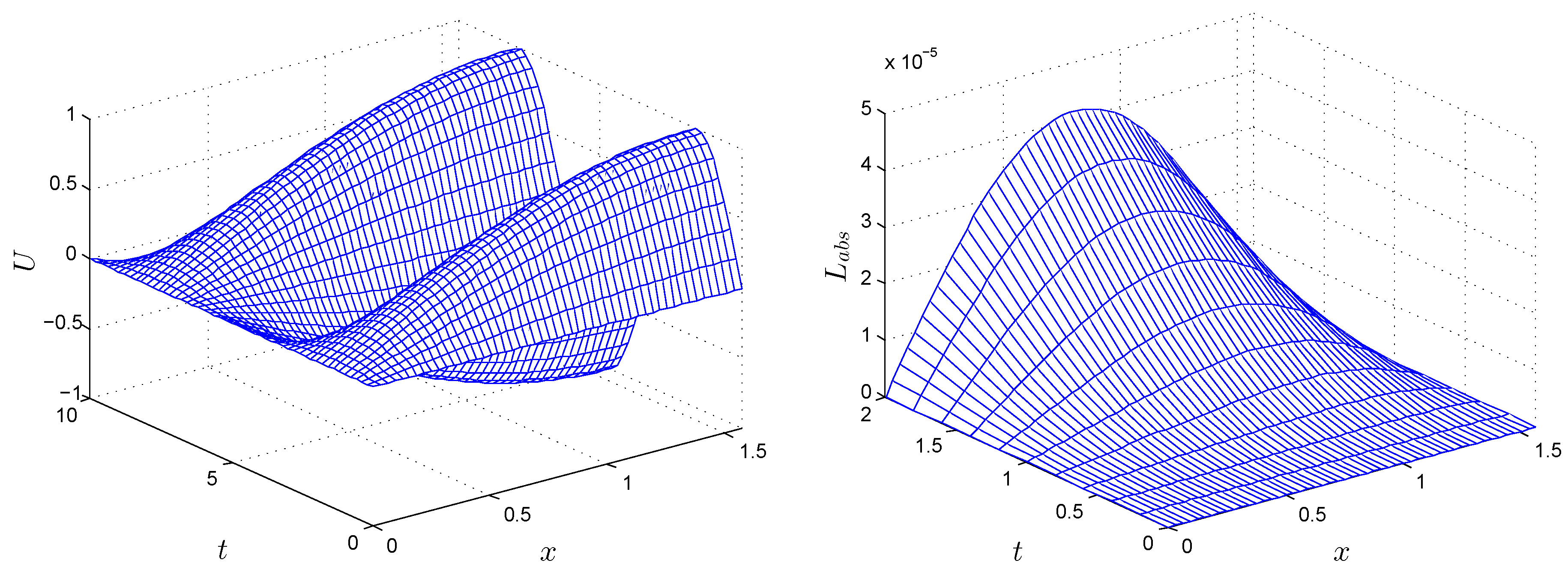
Figure 6 (left) shows the numerical solution with $N=51$, $[0,\pi /2]$, $\Delta t=0.0001$ at various times up to $t=10$, whereas Figure 6 (right) shows the $L_{abs}$ error norm obtained by the FEDF for Test Problem 2.

One of the drawbacks of meshless methods using shape parameter-dependent RBFs is the sensitivity of the shape parameter value. The comparison of both the local and global version of the meshless method for Test Problem 2 is shown in Figure 7. The results were obtained for MQ RBF using $N=41$ and $t=1$. It is clear from Figure 7 that the LMM gave stable results for a long range of shape parameter value c as compared to the GMM.

Figure 8 illustrates the convergence rate of the proposed meshless method in which one can see that the error decreased with the decrease of both the time step size $\Delta t$, as well as the distance between nodes $\Delta x$. Table 5 and Table 6 show the convergence rate corresponding to Test Problem 1. A faster spatial convergence rate as compared to the time convergence rate is verified in this case, as well.

Test Problem 3.

In the third test problem, consider Equation (1) with $h(x,t)=-x\cos \left(t\right)+x^2{\cos }^2\left(t\right)$ and $\alpha =-1$$\beta =0$, $\gamma =1$ with the exact solution given in [38].

$$U(x,t)=x\cos \left(t\right),$$

(32)

with initial conditions:

$$U(x,0)=x,U_t(x,0)=0.$$

(33)

Using the substitution $U_t=V$, we get:

$$U_t=V,V_t=U_{xx}-U^2-x\cos \left(t\right)+x^2{\cos }^2\left(t\right).$$

(34)

Numerical results for different values of t, $[-1,1]$, $N=11$, $\Delta t=0.0001$ are presented in

Table 7. Comparison of the $L_{\infty }$ and $L_2$ error norms for Test Problem 3.

t	1	3	5	7	10
FEDF, $N=11$
$L_{\infty }$	3.3468 × ${10}^{-6}$	6.1312 × ${10}^{-6}$	6.8303 × ${10}^{-6}$	6.3888 × ${10}^{-6}$	5.1932 × ${10}^{-6}$
$L_2$	2.1690 × ${10}^{-6}$	4.2790 × ${10}^{-6}$	5.4027 × ${10}^{-6}$	5.1245 × ${10}^{-6}$	4.4432 × ${10}^{-6}$
Lattice Boltzmann method [10], $N=100$
$L_{\infty }$	1.9558 × ${10}^{-3}$	1.3664 × ${10}^{-3}$	1.5260 × ${10}^{-3}$	1.6201 × ${10}^{-3}$	1.0465 × ${10}^{-3}$
$L_2$	1.1135 × ${10}^{-3}$	7.6676 × ${10}^{-3}$	8.5602 × ${10}^{-3}$	9.5926 × ${10}^{-3}$	6.9848 × ${10}^{-3}$
TPSRBFs method [5], $N=100$
$L_{\infty }$	1.2540 × ${10}^{-5}$	1.5554 × ${10}^{-5}$	3.3792 × ${10}^{-5}$	3.7753 × ${10}^{-5}$	…
$L_2$	6.5422 × ${10}^{-5}$	1.1717 × ${10}^{-4}$	2.2011 × ${10}^{-4}$	2.5892 × ${10}^{-4}$	…
MQ quasi-interpolation scheme [11], $N=10$
$L_{\infty }$	1.25905	1.5428 × ${10}^{-5}$	3.3625 × ${10}^{-5}$	3.7412 × ${10}^{-5}$	…
$L_2$	2.0694 × ${10}^{-5}$	3.7065 × ${10}^{-5}$	6.9684 × ${10}^{-5}$	8.1943 × ${10}^{-5}$	…

, which shows the better performance of the LMM in comparison to the results reported in [5,10,11].

Figure 9 (left) shows the numerical simulation of Test Problem 3, taking $[-1,1]$, $N=51$, $\Delta t=0.0001$, and time up to $t=20$, and Figure 9 (right) shows the $L_{abs}$ error norm by taking $[-1,1]$, $N=101$, $\Delta t=0.0001$, and $t=2$.

In Figure 10, we compare the sensitivity of shape parameter value c for both meshless methods, local and global. It is clear from the figure that the LMM gave stable results in the range $c\in (0,100)$, but on the other hand, the GMM gave stable results only in the range $c\in (0,0.18)$. Figure 11 shows the condition number $\kappa$ versus shape parameter c and number of nodal points N, which is self explanatory.

Test Problem 4.

The exact solutions for the 2D coupled Burgers’ Equation (3) are written as [12,14]:

$$\begin{array}{c}\hfill U(x,y,t)=\frac{3}{4}-\frac{1}{4\left(1+\exp \left((-4x+4y-t)(Re/32)\right)\right)},\\ \hfill V(x,y,t)=\frac{3}{4}+\frac{1}{4\left(1+\exp \left((-4x+4y-t)(Re/32)\right)\right)}.\end{array}$$

(35)

In

Table 8. Comparison of the numerical results of the 2D coupled Burgers’ equation for Test Problem 4.

		U				V
N/$Re$		1	20	100		1	20	100
121	FEDF	1.3 × ${10}^{-8}$	8.5 × ${10}^{-5}$	7.3 × ${10}^{-3}$		3.1 × ${10}^{-8}$	8.5 × ${10}^{-5}$	7.3 × ${10}^{-3}$
	LMAPS [15]	7.4 × ${10}^{-6}$	9.7 × ${10}^{-5}$	7.4 × ${10}^{-3}$		1.0 × ${10}^{-5}$	8.8 × ${10}^{-5}$	7.4 × ${10}^{-3}$
	LDQ [15]	1.4 × ${10}^{-5}$	6.7 × ${10}^{-5}$	7.3 × ${10}^{-3}$		1.9 × ${10}^{-5}$	7.5 × ${10}^{-5}$	7.3 × ${10}^{-3}$
441	FEDF	3.4 × ${10}^{-9}$	2.1 × ${10}^{-5}$	2.0 × ${10}^{-3}$		8.0 × ${10}^{-9}$	2.1 × ${10}^{-5}$	2.0 × ${10}^{-3}$
	LMAPS [15]	1.9 × ${10}^{-6}$	2.4 × ${10}^{-5}$	2.1 × ${10}^{-3}$		2.6 × ${10}^{-6}$	2.1 × ${10}^{-5}$	2.0 × ${10}^{-3}$
	LDQ [15]	3.4 × ${10}^{-6}$	1.7 × ${10}^{-5}$	2.0 × ${10}^{-3}$		4.7 × ${10}^{-6}$	1.9 × ${10}^{-5}$	2.0 × ${10}^{-3}$
961	FEDF	5.6 × ${10}^{-9}$	9.5 × ${10}^{-6}$	8.4 × ${10}^{-4}$		6.4 × ${10}^{-9}$	9.3 × ${10}^{-6}$	8.4 × ${10}^{-4}$
	LMAPS [15]	8.3 × ${10}^{-7}$	1.1 × ${10}^{-5}$	8.5 × ${10}^{-4}$		1.1 × ${10}^{-6}$	9.2 × ${10}^{-6}$	8.4 × ${10}^{-4}$
	LDQ [15]	1.5 × ${10}^{-6}$	7.5 × ${10}^{-6}$	8.4 × ${10}^{-4}$		2.1 × ${10}^{-6}$	8.1 × ${10}^{-6}$	8.2 × ${10}^{-4}$

, the numerical results were obtained by the LMM in terms of the $L_{\infty }$ error norm for Test Problem 4 using the IQ radial basis function with $c=20$. We have used different N and $Re$ and $\Delta t=0.0001$, $t=0.5$. In this table, we have compared the numerical results of the proposed Local meshless method with the local method of approximate particular solutions (LMAPS) [15] and the local RBF-based DQmethod (LDQ) [15]. A full agreement between the results of the LMM and the methods reported in [15] has been observed.

In

Table 9. Comparison of the 2D coupled Burgers’ equation by using the FEDF for Test Problem 4.

	U				V
$(x,y)$	$(0.1,0.1)$	$(0.3,0.3)$	$(0.5,0.5)$		$(0.1,0.1)$	$(0.3,0.3)$	$(0.5,0.5)$
Exact	0.500482	0.500482	0.500482		0.999518	0.999518	0.999518
FEDF	0.500470	0.500443	0.500417		0.999530	0.999557	0.999583
Global RBFs method [14]	0.50035	0.50042	0.50046		0.99936	0.99951	0.99958
Eulerian-Lagrangian method [13]	0.50012	0.50042	0.50041		0.99946	0.99938	0.99941
Finite difference method [12]	0.49983	0.49977	0.49973		0.99826	0.99861	0.99821

, the performance of the LMM for Test Problem 4 is shown against the other methods [12,13,14] at selected points by letting $Re=100$ and $\Delta t=0.0001$, $t=2$, $N=20\times 20$. These results show the accuracy and stable performance of the LMM.

Numerical solutions of the LMM corresponding to Test Problem 4 are shown in Figure 12, Figure 13, Figure 14 and Figure 15 at different Reynolds numbers. It is clear from the figures that up to $Re=300$, the proposed methods can handle the coupled Burgers’ equation, but when we increased Reynolds number, the result became unstable. In contrast, the LMM combined with the upwind technique showed stable results at $Re=1000$, and this phenomena can be seen in Figure 15.

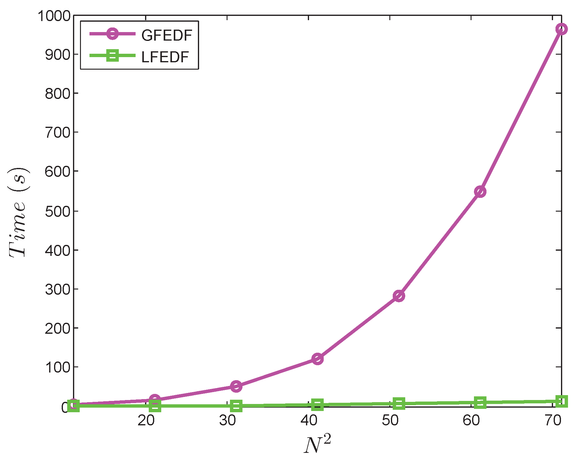
To show the computational efficiency of the LMM over the GMM, we have done a CPU time (in seconds) comparison, which is shown in Figure 16.

Test Problem 5.

Finally, consider the 2D nonlinear RLW Equation (5) with the following exact solution:

$$U(x,y,t)=\frac{q}{2}sec{h}^2\left(\frac{\sqrt{q}}{2p}(x+y-vt-x_0-y_0)\right),$$

(36)

where $q=\frac{6(v-2)}{2}$ and $p=\sqrt{6v}$.

The numerical results and CPU time for Test Problem 5 for $v=2.06$, $N=50$, $\Delta t=0.5$, $[-80,100]$, and up to time $t=20$ are shown in

Table 10. $L_{\infty }$ error norm and CPU time for Test Problem 5.

$\mathit{t}=1$	$\mathit{t}=5$	$\mathit{t}=10$	$\mathit{t}=15$	$\mathit{t}=20$
$L_{\infty }$
6.8814 × ${10}^{-4}$	3.4458 × ${10}^{-3}$	7.0255 × ${10}^{-3}$	1.2374 × ${10}^{-2}$	2.0904 × ${10}^{-2}$
CPU time (in seconds)
2.54	2.59	2.71	2.85	2.88

. This table makes evident that the LMM is an accurate and efficient.

In Figure 17, the $L_{abs}$ error is shown at $t=10$.

Eliminating the requirement of meshing and approximating the solution using uniform or scattered points in rectangular, as well non-rectangular domains is one of the salient features of the LMM. Numerical results of the RLW equation on non-rectangular domains are shown in Figure 18 and Figure 19. The $L_{\infty }$ error norm of the LMM in the computational domain shown in Figure 18 (left) and Figure 19 (left) was $6.8814\times {10}^{-4}$ and $1.7631\times {10}^{-3}$, respectively, at time $t=1$.

4. Conclusions

In the present work, the local meshless method based on RBFs was applied to the 1D Klein–Gordon, 2D coupled Burgers’, and 2D regularized long wave equations. To check the accuracy and efficacy of the proposed scheme on both rectangular and non-rectangular domains, different test problems have been considered. The results of the local meshless method were compared with the exact/approximate solutions available in the existing literature. The stable results (in the case of a high Reynolds number) of the LMM combined with the upwind technique strongly supported the advantage of the LMM over other conventional methods. The LMM has been found to be a flexible interpolation method, as it removes the sensitivity of the shape parameter and produces a well-conditioned coefficient matrix.

References

- Wazwaz, M.A. New travelling wave solutions to the Boussinesq and the Klein–Gordon equations. Commun. Nonlinear Sci. Numer. Simul. 2008, 13, 889–901. [Google Scholar] [CrossRef]
- El-Sayed, S.M. The decomposition method for studying the Klein–Gordon equation. Chaos Soliton Fract. 2003, 18, 1025–1030. [Google Scholar] [CrossRef]
- Duncan, D.B. Symplectic finite difference approximations of the nonlinear Klein–Gordon equation. SIAM J. Numer. Anal. 1997, 34, 1742–1760. [Google Scholar] [CrossRef]
- Lee, I.J. Numerical solution for nonlinear Klein–Gordon equation by collocation method with respect to spectral method. J. Korean Math. Soc. 1995, 32, 541–551. [Google Scholar]
- Dehghan, M.; Shokri, A. Numerical solution of the nonlinear Klein–Gordon equation using radial basis functions. J. Comput. Appl. Math. 2009, 230, 400–410. [Google Scholar] [CrossRef] [Green Version]
- Lakestani, M.; Dehghan, M. Collocation and finite difference-collocation methods for the solution of nonlinear Klein–Gordon equation. Comput. Phys. Commun. 2010, 181, 1392–1401. [Google Scholar] [CrossRef]
- Pekmen, B.; Tezer-Sezgin, M. Differential quadrature solution of nonlinear Klein–Gordon and Sine-Gordon equations. Comput. Phys. Commun. 2012, 183, 1702–1713. [Google Scholar] [CrossRef]
- Hariharan, G. Haar wavelet method for solving the Klein–Gordon and the Sine-Gordon equations. Int. J. Nonlinear Sci. 2011, 11, 180–189. [Google Scholar]
- Yin, F.; Song, J.; Lu, F. A coupled method of Laplace transform and Legendre wavelets for nonlinear Klein–Gordon equations. Math. Methods Appl. Sci. 2014, 37, 781–791. [Google Scholar] [CrossRef]
- Li, Q.; Ji, Z.; Zheng, Z.; Liu, H. Numerical solution of nonlinear Klein–Gordon equation using Lattice Boltzmann method. Appl. Math. 2011, 2, 1479–1485. [Google Scholar] [CrossRef]
- Sarboland, M.; Aminataei, A. Numerical solution of the nonlinear Klein–Gordon equation using multiquadric quasi-interpolation scheme. Univ. J. Math. Appl. 2015, 3, 40–49. [Google Scholar]
- Bahadir, A.R. A fully implicit finite difference scheme for two-dimensional Burgers’ equations. Appl. Math. Comput. 2003, 137, 131–137. [Google Scholar] [CrossRef]
- Younga, D.; Fana, C.; Hua, S.; Atluri, S. The Eulerian-Lagrangian method of fundamental solutions for two-dimensional unsteady Burgers’ equations. Eng. Anal. Bound. Elem. 2009, 32, 395–412. [Google Scholar] [CrossRef]
- Ali, A.; Siraj-ul-Islam; Haq, S. A computational meshfree technique for the numerical solution of the two-dimensional coupled Burgers’ equations. Int. J. Comput. Meth. Eng. Sci. Mech. 2009, 10, 406–412. [Google Scholar] [CrossRef]
- Zhang, X.; Zhu, H.; Kuo, L. A comparison study of the LMAPS method and the LDQ method for time-dependent problems. Eng. Anal. Bound. Elem. 2013, 37, 1408–1415. [Google Scholar] [CrossRef]
- Dehghan, M.; Salehi, R. The solitary wave solution of the two-dimensional regularized long-wave equation in fluids and plasmas. Comput. Phys. Commun. 2011, 182, 2540–2549. [Google Scholar] [CrossRef]
- Dehghana, M.; Abbaszadeha, M.; Mohebbib, A. The use of interpolating element-free Galerkin technique for solving 2D generalized Benjamin-Bona-Mahony-Burgers and regularized long-wave equations on non-rectangular domains with error estimate. J. Comput. Appl. Math. 2015, 286, 211–231. [Google Scholar] [CrossRef]
- Abdulloev, K.O.; Bogolubsky, I.L.; Makhankov, V.G. One more example of inelastic soliton interaction. Phys. Lett. 1976, 56A, 427–428. [Google Scholar] [CrossRef]
- Bona, J.L.; Bryant, P.J. A mathematical model for long waves generated by wave makers in nonlinear dispersive systems. Proc. Camb. Philos. Soc. 1973, 73, 391–405. [Google Scholar] [CrossRef]
- Bhardwaj, D.; Shankar, R. A computational method for regularized long wave equation. Comput. Math. Appl. 2000, 40, 1397–1404. [Google Scholar] [CrossRef] [Green Version]
- Esen, A.; Kutluay, S. Application of a lumped Galerkin method to the regularized long wave equation. Appl. Math. Comput. 2006, 174, 833–845. [Google Scholar] [CrossRef]
- Gou, B.Y.; Cao, W.M. The Fourier pseudospectral method with a restrain operator for the RLW equation. Comput. Math. Appl. 1988, 74, 110–126. [Google Scholar]
- Raslan, K.R. A computational method for the regularized long wave equation. Appl. Math. Comput. 2005, 167, 1101–1118. [Google Scholar] [CrossRef]
- Roshan, T. A Petrov-Galerkin method for solving the generalized regularized long wave (GRLW) equation. Comput. Math. Appl. 2012, 63, 943–956. [Google Scholar] [CrossRef]
- Guo, P.F.; Zhang, L.W.; Liew, K.M. Numerical analysis of generalized regularized long wave equation using the element-free kp-Ritz method. Appl. Math. 2014, 240, 91–101. [Google Scholar] [CrossRef]
- Shen, Q. Local RBF-based differential quadrature collocation method for the boundary layer problems. Eng. Anal. Bound. Elem. 2010, 34, 213–228. [Google Scholar] [CrossRef]
- Ahsan, M.; Ahmad, I.; Ahmad, M.; Hussian, A. A numerical Haar wavelet-finite difference hybrid method for linear and non-linear Schrödinger equation. Math. Comput. Simul. 2019. [Google Scholar] [CrossRef]
- Thounthong, P.; Khan, M.; Hussain, I.; Ahmad, I.; Kumam, P. Symmetric Radial Basis Function Method for Simulation of Elliptic Partial Differential Equations. Mathematics 2018, 6, 327. [Google Scholar] [CrossRef]
- Kudela, H.; Malecha, Z.M. Eruption of a boundary layer induced by a 2D vortex patch. Fluid Dyn. Res. 2009, 41, 055502. [Google Scholar] [CrossRef]
- Seydaoğlu, M. A Meshless Method for Burgers’ Equation Using Multiquadric Radial Basis Functions with a Lie-Group Integrator. Mathematics 2019, 7, 113. [Google Scholar] [CrossRef]
- Shen, Q. Numerical solution of the Sturm-Liouville problem with local RBF-based differential quadrature collocation method. Int. J. Comput. Math. 2011, 88, 285–295. [Google Scholar] [CrossRef]
- Siraj-ul-Islam; Ahmad, I. A comparative analysis of local meshless formulation for multi-asset option models. Eng. Anal. Bound. Elem. 2016, 65, 159–176. [Google Scholar]
- Siraj-ul-Islam; Ahmad, I. Local meshless method for PDEs arising from models of wound healing. Appl. Math. Model. 2017, 48, 688–710. [Google Scholar]
- Ahmad, I.; Siraj-ul-Islam; Khaliq, A.Q.M. Local RBF method for multi-dimensional partial differential equations. Comput. Math. Appl. 2017, 74, 292–324. [Google Scholar] [CrossRef]
- Ahmad, I.; Riaz, M.; Ayaz, M.; Arif, M.; Islam, S.; Kumam, P. Numerical Simulation of Partial Differential Equations via Local Meshless Method. Symmetry 2019, 11, 257. [Google Scholar] [CrossRef]
- Ahmad, I.; Ahsan, M.; Zaheer-ud-Din; Ahmad, M.; Kumam, P. An Efficient Local Formulation for Time-Dependent PDEs. Mathematics 2019, 7, 216. [Google Scholar] [CrossRef]
- Ahmad, I. Local Meshless Collocation Method for Numerical Solution of Partial Differential Equations. Ph.D. Thesis, University of Engineering and Technology, Peshawar, Pakistan, 2017. [Google Scholar]
- Hussain, A.; ul Haq, S.; Uddin, M. Numerical solution of Klein–Gordon and sine-Gordon equations by meshless method of lines. Eng. Anal. Bound. Elem. 2013, 37, 1351–1366. [Google Scholar] [CrossRef]
- Khuri, S.; Sayfy, A. A spline collocation approach for the numerical solution of a generalized nonlinear Klein–Gordon equation. Appl. Math. Comput. 2010, 216, 1047–1056. [Google Scholar] [CrossRef]
Figure 1.
Schematics of the local supported domain in 2D geometry for [34].
Figure 2.
Schematic of the local supported domain in 2D geometry for in the upwind technique [34].
Figure 3.
Numerical and exact solutions for with for Test Problem 1.
Figure 4.
c versus the error norm of the local meshless method (LMM) (left) and the global meshless method (GMM) (right) for Test Problem 1.
Figure 5.
Convergence in space (left) and convergence in time (right) for Test Problem 1.
Figure 6.
Numerical simulation (left) and (right) for Test Problem 2.
Figure 7.
c versus the error norm of the LMM (left) and GMM (right) for Test Problem 2.
Figure 8.
Convergence in space (left) at and convergence in time (right) at for the test problem 2.
Figure 9.
Numerical simulation (left) and (right) for the Test Problem 3.
Figure 10.
c versus the error norm of the LMM (left) and GMM (right) for Test Problem 3.
Figure 11.
c versus (left) and the number of nodal points N versus (right) of the LMM for Test Problem 3.
Figure 12.
Numerical solution of the 2D coupled Burgers’ with , , for Test Problem 4.
Figure 13.
Numerical solution of the 2D coupled Burgers’ with , for Test Problem 4.
Figure 14.
Numerical solution of the 2D coupled Burgers’ combined with the upwind technique for , for Test Problem 4.
Figure 15.
Figure 16.
Comparison of the CPU time of the LMM and the GMM with , for Test Problem 4.
Figure 17.
error norm of the LMM for Test Problem 5.
Figure 18.
Computational domains (left) and numerical results (right) for Test Problem 5.
Figure 19.