Lie and Q-Conditional Symmetries of Reaction-Diffusion-Convection Equations with Exponential Nonlinearities and Their Application for Finding Exact Solutions

Abstract

This review is devoted to search for Lie and Q-conditional (nonclassical) symmetries and exact solutions of a class of reaction-diffusion-convection equations with exponential nonlinearities. A complete Lie symmetry classification of the class is derived via two different algorithms in order to show that the result depends essentially on the type of equivalence transformations used for the classification. Moreover, a complete description of Q-conditional symmetries for PDEs from the class in question is also presented. It is shown that all the well-known results for reaction-diffusion equations with exponential nonlinearities follow as particular cases from the results derived for this class of reaction-diffusion-convection equations. The symmetries obtained for constructing exact solutions of the relevant equations are successfully applied. The exact solutions are compared with those found by means of different techniques. Finally, an application of the exact solutions for solving boundary-value problems arising in population dynamics is presented.

1. Introduction

It is well known that nonlinear evolution PDEs play a crucial role in mathematical modeling of a wide range of processes in natural, social and life sciences. Power-law nonlinearities are the most common in real-world applications. Nonlinear evolution PDEs with such nonlinearities have been studied by different mathematical techniques (including the symmetry-based methods) since the beginning of the 20th Century. The classical example is the porous-medium equation:

$$u_t={(u{u}_x)}_x$$

(1)

(hereafter, $u=u(t,x)$ is an unknown function, and the lower subscripts t and x denote differentiation with respect to these variables), which was studied by J.Boussinesq in order to describe the solute filtration in soil [1]. Two other well-known examples of the evolution PDEs with power-law nonlinearities are the fast-diffusion equation:

$$u_t={(u^{-2}{u}_x)}_x,$$

(2)

which was introduced in [2], and the celebrated Burgers equation [3]:

$$u_t=u_{xx}+u{u}_x.$$

(3)

Notably, Equations (2) and (3) are linearizable [2,4,5,6] (see more details about symmetries and exact solutions of the second-order evolution PDEs with power-law nonlinearities in our recent book [7]).

In contrast to the evolution PDEs with power-law nonlinearities, there are not many papers devoted to the examination of reaction-diffusion-convection (RDC) equations with exponential nonlinearities. To the best of our knowledge, the first examples of real-world models based on such equations were proposed by D. Frank-Kamenetskii and H. Fujita [8,9] (see also earlier references cited therein). The corresponding equation is:

$$u_t=u_{xx}+e^u$$

(4)

and one describes some heat and chemical processes (in particular, combustion processes). The Lie symmetry of Equation (4) is the three-dimensional Lie algebra [10]. Notably, the well-known RD equation with the Arrhenius reaction term $e^{-A_0/u}$ ($A_0$ is a positive constant), which is widely used in applications, can be reduced to the form (4) (with $e^u\to \exp (A_0^{\ast }u-u_0),A_0^{\ast }>0,u_0>0$) via a corresponding approximation (see, for details, [11]).

The first appearance of a PDE with the exponential nonlinearity in the diffusion coefficient probably was in the Ovsiannikov paper [12] devoted to the Lie symmetry classification (LSC) of nonlinear diffusion equations. This equation has the form:

$$u_t={(e^u{u}_x)}_x$$

(5)

and is invariant with respect to the four-dimensional Lie algebra.

There are some recent papers devoted to the study of the evolution PDEs with the exponential nonlinearity by different mathematical methods (see, e.g., [13,14,15] and the references cited therein).

In this review, we unite all the known results about Lie and Q-conditional symmetry, exact solutions and their applications for the following class of RDC equations:

$$u_t={(e^{nu}{u}_x)}_x+\lambda e^{mu}{u}_x+C(u),$$

(6)

where $n,m$ and $\lambda$ are arbitrary constants. Moreover, we present some new results. Our aim is to discuss only such equations of the form (6), which contain exponential nonlinearities in the diffusion, reaction and/or convection term(s). We note from the very beginning that the case $m=0$ is special because Equation (6) is reducible to the reaction-diffusion equation:

$$u_t={(e^{nu}{u}_y)}_y+C(u)$$

by the substitution $y=x+\lambda t$ (the Galilei boost); hence, it is assumed $m\ne 0$ in what follows.

The review is organized as follows. In Section 2, the LSC of the class of RDC Equation (6) is presented using two different approaches. Firstly, we apply the well-known Lie–Ovsiannikov algorithm based on equivalence transformations (ETs), and afterwards, we apply a modern LSC algorithm based on form-preserving (admissible) transformations (FPTs). In Section 3, Lie’s (invariant) solutions of some equations from class (6) are constructed using the Lie symmetries derived in Section 2. Section 4 is devoted to the search for Q-conditional (nonclassical) symmetries of (6). In Section 5, a wide range of non-Lie solutions (i.e., such exact solutions, which are not obtainable via Lie symmetries) are derived for two RDC equations of the form (6). Section 6 contains an application of the results to population dynamics. In the last section, we present some conclusions and highlight new results obtained in this review.

2. Lie Symmetry

In this section, we discuss the Lie symmetry of the class of RDC Equation (6). This means that the LSC problem should be solved, i.e., to describe all possible forms of $C(u)$ corresponding to different algebras of invariance. Ovsiannikov was the first to solve this problem for PDEs [12]; simultaneously, he created an approach (called the Lie–Ovsiannikov algorithm) that allows us to solve such kinds of problems for other classes of PDEs [16]. Following Ovsiannikov’s works, the LSC problem is often called the group classification problem. We think that this terminology is misleading (especially for the reader who is not a specialist in symmetry-based methods) because the algorithm allows us to find Lie algebras for PDEs. Having a complete list of the Lie algebras for a given PDE class, of course, one may easily construct all the corresponding Lie groups.

The problem LSC is solved for the given PDE class via the Lie–Ovsiannikov algorithm if it has been proven that:

(1)

the Lie symmetry algebras are maximal algebras of invariance (MAIs) of the relevant PDEs from the list obtained;

(2)

all PDEs from the list are inequivalent with respect to a set of ETs;

(3)

any other PDE from the class that admits a nontrivial Lie symmetry algebra is reduced by an ET from the set to one of those from the list.

Let us introduce a definition of the continuous ETs.

Definition 1.

([7,17]) A one-parameter group of ETs of the class of k-order PDEs:

$$L(t,x,u,\underset{1}{u},\cdots ,\underset{k}{u},K_1,\cdots ,K_p)=0,$$

(7)

where L is a given smooth function of their arguments (here $K_1,\cdots ,K_p$ are some functions (parameters), which may depend on $t,x,u$ and/or derivatives of u, while $\underset{k}{u}$ means a totality of k-order derivatives of $u(t,x)$) and is the one-parameter Lie group of transformations given by:

$$\begin{array}{c}\overline{t}=f(t,x,u,ϵ),{\overline{x}}_a=g_a(t,x,u,ϵ),a=1,\cdots ,n,\overline{u}=h(t,x,u,ϵ),\\ {\overline{K}}_i=F_i(t,x,u,K_1,\cdots ,K_p,ϵ),i=1,\cdots ,p\end{array}$$

where $x=(x_1,\cdots ,x_n)$ and ϵ is the group parameter, which maps each equation of the form (7) into an equation belonging to the same class.

Definition 2.

The group $\mathcal{E}$ is called the group of ETs for the PDE class (7), if $\mathcal{E}$ contains as subgroups all one-parameter groups of ETs of this class.

It is worth noting that it follows immediately from Definition 2 that the group $\mathcal{E}$ is larger for a wider class of PDEs (i.e., its dimensionality is higher). In particular, the general class of RDC equations:

$$u_t={[D(u)u_x]}_x+K(u)u_x+C(u)$$

(8)

admits the group $\mathcal{E}$, which is the seven-parameter Lie group:

$$\begin{array}{c}\overline{t}=e_{0}t+t_0,\overline{x}=e_{1}x+gt+x_0,\overline{u}=e_{2}u+u_0,\\ \overline{D}=\frac{e_1^2}{e_0}D,\overline{K}=\frac{e_1}{e_0}K,\overline{C}=\frac{1}{e_0}C,\end{array}$$

where $e_i(i=0,1,2),t_0,x_0,g$ and $u_0$ are arbitrary group parameters ($e_i>0$).

It can be proven that the group $\mathcal{E}$ of the class of PDEs (6) is only the five-parameter Lie group.

Theorem 1.

The group of the continuous ETs of the class of RDC Equation (6) is the five-parameter Lie group:

$$\begin{array}{c}\overline{t}=e_{0}t+t_0,\overline{x}=e_{1}x+x_0,\overline{u}=e_{2}u+u_0,\overline{C}=\frac{e_2}{e_0}C,\\ \overline{n}=\frac{1}{e_2}n,\overline{m}=\frac{1}{e_2}m,\overline{\lambda }=\frac{e_1}{e_0}\exp (-\frac{m{u}_0}{e_2})\lambda ,\end{array}$$

(9)

where $e_0=e_1^2\exp (-\frac{n{u}_0}{e_2})$, $t_0,x_0,e_1$ and $e_2$ are arbitrary group parameters ($e_1>0,e_2>0$).

Remark 1.

The class of PDEs (6) is also invariant with respect to the discrete transformation:

$$\overline{x}=-x,\overline{u}=-u,$$

(10)

hence we assume that $e_1\ne 0$ and $e_2\ne 0$ in

Table 1. The complete Lie symmetry classification (LSC) of equations of the form (6) using the group $\mathcal{E}$. MAI, maximal algebras of invariance.

	RDC Equations	MAI	Constraints
1	$u_t={(e^u{u}_x)}_x$	$<{\partial }_t,{\partial }_x,D_0,D_2>$
2	$u_t={(e^u{u}_x)}_x+p$	$<{\partial }_t,{\partial }_x,T,D_2>$	$p=\pm 1$
3	$u_t={(e^u{u}_x)}_x+e^u{u}_x+\frac{2}{9}{e}^u$	$<{\partial }_t,{\partial }_x,D_1,X>$
4	$u_t={(e^u{u}_x)}_x+e^u{u}_x+\frac{2}{9}{e}^u+p$	$<{\partial }_t,{\partial }_x,T,X>$	$p=\pm 1$
5	$u_t={(e^u{u}_x)}_x+{\lambda }_3{e}^u{u}_x+{\lambda }_6{e}^u+p$	$<{\partial }_t,{\partial }_x,T>$	$|{\lambda }_3|+|{\lambda }_6|\ne 0,{\lambda }_6\ne \frac{2}{9}{\lambda }_3^2,p=\pm 1$
6	$u_t={(e^{nu}{u}_x)}_x+{\lambda }_2{e}^{mu}{u}_x+{\lambda }_3{e}^{(2m-n)u}$	$<{\partial }_t,{\partial }_x,(n-2m)D_0+D_2>$	$|{\lambda }_2|+|{\lambda }_3|\ne 0$

and in what follows.

In order to obtain LSC of (6), one needs to find the so-called principal Lie group from the very beginning.

Definition 3.

([7]) A Lie group, which is the invariance group for all equations belonging to the PDE class (7) and contains as a subgroup any other Lie group that is common for all PDEs from this class, is called the principal Lie group (another terminology is “kernel of main groups”). The corresponding Lie algebra is called the principal algebra of the class in question.

It can be easily shown using Theorem 1 that the principal Lie algebra of (6) is the two-dimensional algebra with the basic operators ${\partial }_t$ and ${\partial }_x$. These operators generate the two-dimensional Lie group of time and space translations. Because this algebra occurs for all smooth functions $C(u)$, this case is omitted in what follows.

Theorem 2.

([18]) All possible MAIs of RDC equations of the form (6) depending on the function $C(u)$ are presented in Table 1. Any other equation of the form (6) with nontrivial Lie symmetry (i.e., its MAI is of dimensionality three and higher) is reduced by an ET from $\mathcal{E}$ (9) to one of six equations listed in Table 1.

Proof of this theorem immediately follows from LSC of the class of PDEs (8) derived in [18].

Remark 2.

In Table 1, the following designations for Lie symmetry operators are introduced:$D_0=2t{\partial }_t+x{\partial }_x,D_1=t{\partial }_t-{\partial }_u,D_2=nx{\partial }_x+2{\partial }_u,T=e^{-pt}({\partial }_t+p{\partial }_u),X=e^{-\frac{1}{3}x}({\partial }_x-\frac{2}{3}{\partial }_u).$

During the last two decades, new approaches for solving LSC problems were developed. The most known among them is the method that is based on the so-called FPTs [19,20]. FPTs were used initially for finding locally-equivalent PDEs, especially those nonlinear PDEs that are linearizable by a point transformation (i.e., a non-generating transformation, which does not involve derivatives of unknown function(s)). It is worth noting that these transformations are called also “admissible transformations” following the 1992 paper [21], in which they were used to classify the Lie symmetries of a class of variable coefficient Korteweg–de Vries equations. Interestingly, such transformations were implicitly used much earlier in the 1978 paper [22] in order to find all possible heat equations with nonlinear sources that admit the Lie symmetry either of the linear heat equation or of the Burgers equation.

It should be stressed that FPTs allow us an essential reduction of the number of cases obtained via the Lie–Ovsiannikov algorithm (see, e.g., extensive discussions on this matter in [23,24,25]). For example, it was proven using a set of FPTs that the canonical list of inequivalent two-component systems of RD equations (with a nonconstant diffusivity) admitting a non-trivial Lie symmetry consists of 10 systems only [24] (not the approximately 30 systems derived by the Lie–Ovsiannikov algorithm in [26]).

Here, we show below that a similar reduction of the number of different cases occurs also with Equation (6).

Definition 4.

A point non-degenerate transformation given by:

$$\tau =a(t,x,u),y=b(t,x,u),w=c(t,x,u),$$

(11)

which maps at least one equation of the form (7) into an equation belonging to the same class, is called the FPT for the PDE class (7).

Comparing this definition with Definition 2, one immediately notes that each ET from $\mathcal{E}$ is automatically a FPT, but not vice versa. In contrast to the ETs, a set of all possible FPTs for the given class of PDEs usually does not form a Lie group. However, a subset of FPTs may generate a group of ETs on a subclass of the given class [24]. This is a reason why FPTs are also called additional ETs.

Theorem 3.

A RDC equation from class (6) with $|n|+|\lambda |\ne 0$ can be reduced to another equation from this class:

$$w_{\tau }={(e^{n_{1}w}{w}_y)}_y+{\lambda }_1{e}^{m_{1}w}{w}_y+H(w)$$

by an FPT of the form (11) if and only if the equation has one of the forms listed in the second column of

Table 2. Form-preserving transformations (FPTs) of the class of reaction-diffusion-convection (RDC) Equation (6).

	RDC Equation	FPT	RDC Equation
1	$u_t=u_{xx}+\lambda e^u{u}_x+C(u)$	(12)	$w_{\tau }=w_{yy}+c_2^{-1}\lambda e^w{w}_y+c_0^{-2}C(w-\ln \frac{c_2}{c_0})$
2	$u_t={(e^u{u}_x)}_x+\lambda e^{mu}{u}_x+C(u)$	(13)	$w_{\tau }={(e^w{w}_y)}_y+c_0^{2(m-1)}{c}_1^{1-2m}\lambda e^{mw}{w}_y+c_0^{-2}C(w-\ln \frac{c_1^2}{c_0^2})$
3	$u_t={(e^u{u}_x)}_x+\lambda e^u{u}_x+\frac{2}{9}{\lambda }^2{e}^u$	(14)	$w_{\tau }={(e^w{w}_y)}_y$
4	$u_t={(e^u{u}_x)}_x+\lambda e^u{u}_x+{\lambda }_2{e}^u+{\lambda }_3$	(15)	$w_{\tau }={(e^w{w}_y)}_y+c_1^{-1}\lambda e^w{w}_y+c_1^{-2}{\lambda }_2{e}^w+c_0^{-2}{\lambda }_3$
5	$u_t={(e^u{u}_x)}_x+\lambda e^u{u}_x+{\lambda }_2{e}^u+{\lambda }_3$	(16)	$w_{\tau }={(e^w{w}_y)}_y+c_1^{-1}\lambda e^w{w}_y+c_1^{-2}{\lambda }_2{e}^w$
6	$u_t={(e^u{u}_x)}_x+\lambda e^u{u}_x+\frac{2}{9}{\lambda }^2{e}^u+{\lambda }_3$	(17)	$w_{\tau }={(e^w{w}_y)}_y+c_1^{-1}\lambda e^w{w}_y+\frac{2}{9}{c}_1^{-2}{\lambda }^2{e}^w+c_0^{-2}{\lambda }_3$
7	$u_t={(e^u{u}_x)}_x+\lambda e^u{u}_x+\frac{2}{9}{\lambda }^2{e}^u+{\lambda }_3$	(18)	$w_{\tau }={(e^w{w}_y)}_y+c_1^{-1}\lambda e^w{w}_y+\frac{2}{9}{c}_1^{-2}{\lambda }^2{e}^w$
8	$u_t={(e^u{u}_x)}_x+\lambda e^u{u}_x+\frac{2}{9}{\lambda }^2{e}^u+{\lambda }_3$	(19)	$w_{\tau }={(e^w{w}_y)}_y+c_0^{-2}{\lambda }_3$
9	$u_t={(e^u{u}_x)}_x+\lambda e^u{u}_x+\frac{2}{9}{\lambda }^2{e}^u+{\lambda }_3$	(20)	$w_{\tau }={(e^w{w}_y)}_y$

, while the corresponding FTP in the third column belongs to the following set of transformations:

$$\tau =c_0^{2}t+d_0,y=c_{0}x+d_1,w=u+\ln \frac{c_2}{c_0},c_0{c}_2\lambda \ne 0.$$

(12)

$$\tau =c_0^{2}t+d_0,y=c_{1}x+d_1,w=u+\ln \frac{c_1^2}{c_0^2},c_0{c}_1\ne 0.$$

(13)

$$\tau =c_0^{2}t+d_0,y=c_1{e}^{\frac{\lambda }{3}x}+d_1,w=u+\frac{2\lambda }{3}x+\ln \frac{c_1^2{\lambda }^2}{9c_0^2},c_0{c}_1\lambda \ne 0.$$

(14)

$$\tau =\frac{c_0^2}{{\lambda }_3}\ln (e^{{\lambda }_{3}t}+c_2)+d_0,y=c_{1}x+d_1,w=u+\ln (1+c_2{e}^{-{\lambda }_{3}t})+\ln \frac{c_1^2}{c_0^2},c_0{c}_1{\lambda }_3\ne 0.$$

(15)

$$\tau =\frac{c_0^2}{{\lambda }_3}{e}^{{\lambda }_{3}t}+d_0,y=c_{1}x+d_1,w=u-{\lambda }_{3}t+\ln \frac{c_1^2}{c_0^2},c_0{c}_1{\lambda }_3\ne 0.$$

(16)

$$\begin{array}{c}\tau =\frac{c_0^2}{{\lambda }_3}\ln (e^{{\lambda }_{3}t}+c_3)+d_0,y=\frac{3c_1}{\lambda }\ln (e^{\frac{\lambda }{3}x}+c_2)+d_1,\\ w=u+\ln \left(c_3{e}^{-{\lambda }_{3}t}+1\right)-2\ln \left(c_2{e}^{-\frac{\lambda x}{3}}+1\right)+\ln \frac{c_1^2}{c_0^2},c_0{c}_1\lambda {\lambda }_3\ne 0.\end{array}$$

(17)

$$\begin{array}{c}\tau =\frac{c_0^2}{{\lambda }_3}{e}^{{\lambda }_{3}t}+d_0,y=\frac{3c_1}{\lambda }\ln (e^{\frac{\lambda }{3}x}+c_2)+d_1,w=u-{\lambda }_{3}t-2\ln \left(c_2{e}^{-\frac{\lambda x}{3}}+1\right)+\ln \frac{c_1^2}{c_0^2},\\ c_0{c}_1\lambda {\lambda }_3\ne 0.\end{array}$$

(18)

$$\begin{array}{c}\tau =\frac{c_0^2}{{\lambda }_3}\ln (e^{{\lambda }_{3}t}+c_2)+d_0,y=c_1{e}^{\frac{\lambda }{3}x}+d_1,w=u+\ln \left(c_2{e}^{-{\lambda }_{3}t}+1\right)+\frac{2\lambda }{3}x+\ln \frac{c_1^2{\lambda }^2}{9c_0^2},\\ c_0{c}_1\lambda {\lambda }_3\ne 0.\end{array}$$

(19)

$$\tau =\frac{c_0^2}{{\lambda }_3}{e}^{{\lambda }_{3}t}+d_0,y=c_1{e}^{\frac{\lambda }{3}x}+d_1,w=u-{\lambda }_{3}t+\frac{2\lambda }{3}x+\ln \frac{c_1^2{\lambda }^2}{9c_0^2},c_0{c}_1\lambda {\lambda }_3\ne 0.$$

(20)

Remark 3.

In the case $n=\lambda =0,$ Equation (6) takes the form:

$$u_t=u_{xx}+C(u),$$

(21)

and is reduced, using a transformation of the form (11), to the equation of the same subclass:

$$w_{\tau }=w_{yy}+H(w),$$

if and only if the corresponding FPT has the form:

$$a=\int A^2(t)\mathtt{d}t,b=A(t)x+B(t),c=\alpha (t,x)u+\beta (t,x),$$

(22)

where $\alpha (t,x)=\gamma (t)\exp (-\frac{A^{\prime }}{4A}{x}^2-\frac{B^{\prime }}{2A}x),A\gamma \ne 0,$ and the equality takes place:

$$\alpha C(u)+\left({\alpha }_t-{\alpha }_{xx}+2\frac{{\alpha }_x^2}{\alpha }\right)u+{\beta }_t-{\beta }_{xx}+2\frac{{\alpha }_x{\beta }_x}{\alpha }=b_x^{2}H(\alpha u+\beta ).$$

(23)

In particular, equation:

$$u_t=u_{xx}+{\lambda }_2{e}^u+{\lambda }_3$$

is reduced to the equation:

$$w_{\tau }=w_{yy}+c_2^{-2}{\lambda }_2{e}^w+c_0^{-2}{\lambda }_3,$$

via the transformation:

$$\tau =c_0^{2}t+d_0,y=c_{1}x+d_1,w=u+\ln \frac{c_2^2}{c_0^2}.$$

Proof. 

In order to prove the theorem, we use the result derived in [18] for the general class of RDC Equation (8). Substituting the functions $D(u)=e^{nu},K(u)=\lambda e^{mu},F(w)=e^{n_{1}w}$ and $G(w)={\lambda }_1{e}^{m_{1}w}$ directly into Equations (35)–(37) [18], we immediately obtain:

$$a=a(t),b=b(t,x),c=\alpha (t,x)u+\beta (t,x),a_t{b}_x\alpha \ne 0,$$

while the functions $a(t),b(t,x),\alpha (t,x)$ and $\beta (t,x)$ satisfy the over-determined system:

$$b_x^2{e}^{nu}=a_t{e}^{n_1(\alpha u+\beta )},$$

(24)

$$-2\frac{b_x{\alpha }_x}{\alpha }\frac{d}{du}(u{e}^{nu})-2\frac{n{b}_x{\beta }_x}{\alpha }{e}^{nu}+b_{xx}{e}^{nu}+\lambda b_x{e}^{mu}={\lambda }_1{a}_t{e}^{m_1(\alpha u+\beta )}+b_t,$$

(25)

$$\begin{array}{c}\frac{{\alpha }_x^2}{\alpha }\frac{d}{du}(u^2{e}^{nu})+2\frac{{\alpha }_x{\beta }_x}{\alpha }\frac{d}{du}(u{e}^{nu})+\frac{n{\beta }_x^2}{\alpha }{e}^{nu}-({\alpha }_{xx}u+{\beta }_{xx})e^{nu}-\\ -\lambda ({\alpha }_{x}u+{\beta }_x)e^{mu}+\alpha C(u)+{\alpha }_{t}u+{\beta }_t=a_{t}H(\alpha u+\beta ).\end{array}$$

(26)

Analyzing Equation (24), we derive two different cases, namely $n{n}_1\ne 0$ and $n=n_1=0$.

Let us examine the case $n{n}_1\ne 0$. Using Equation (24) and a relevant ET of the form (9), we obtain:

$$n=n_1=1,\alpha =1,\beta =2\ln b_x-\ln a_t.$$

(27)

Substituting (27) into (25), we arrive at the classification equation:

$$\lambda b_x{e}^{mu}-{\lambda }_1{a}_t^{1-m_1}{b}_x^{2m_1}{e}^{m_{1}u}-3b_{xx}{e}^u-b_t=0,$$

(28)

which leads to the three nonequivalent subcases:

(1)

$\lambda ={\lambda }_1=0,$

(2)

$\lambda {\lambda }_1\ne 0,$

(3)

$\lambda \ne 0,{\lambda }_1=0$

Let us consider Subcase (1) in detail. We immediately obtain from Equation (28) that:

$$b=c_{1}x+d_1.$$

(29)

Substituting (29) and (27) into (26), we arrive at:

$$C(u)=a_{t}H(u+2\ln c_1-\ln a_t)+\frac{a_{tt}}{a_t}.$$

(30)

Differentiating (30) with respect to t, we obtain the equation:

$$a_{tt}(H^{\prime }-H)={\left(\frac{a_{tt}}{a_t}\right)}_t.$$

(31)

Assuming $a_{tt}=0$, i.e., $a=c_0^{2}t+d_0$, after simple calculations, we derive FPT (13) and Case 2 of Table 2 with $\lambda =0$ and $m=1$.

If $a_{tt}\ne 0$, then Equation (31) can be rewritten as two ODEs:

$$H^{\prime }-H=-{\lambda }_4,\frac{1}{a_{tt}}{\left(\frac{a_{tt}}{a_t}\right)}_t=-{\lambda }_4,$$

(32)

where ${\lambda }_4$ is an arbitrary constant.

The solution of the first ODE has the form:

$$H=c_1^{-2}{\lambda }_2{e}^w+{\lambda }_4,$$

while the second ODE is equivalent to the ODE:

$$e^{{\lambda }_{4}a}{a}_t=c_0^2{e}^{{\lambda }_{3}t},$$

(33)

where $c_0^2>0$ because of (24).

The solution of Equation (33) essentially depends on ${\lambda }_3$ and ${\lambda }_4$. There are three subcases:

(a)

$({\lambda }_3,{\lambda }_4)=({\lambda }_3,0),{\lambda }_3\ne 0,$

(b)

$({\lambda }_3,{\lambda }_4)=(0,{\lambda }_4),{\lambda }_4\ne 0,$

(c)

$({\lambda }_3,{\lambda }_4)\ne (0,0).$

In Subcase (a), Equation (33) gives:

$$a=\frac{c_0^2}{{\lambda }_3}{e}^{{\lambda }_{3}t}+d_0.$$

Therefore, taking into account (27) and (29), we obtain Case 5 of Table 2 with $\lambda ={\lambda }_1=0$.

Subcase (b) leads to:

$$a=\frac{1}{{\lambda }_4}\ln (t+c_1)+d_0.$$

It can be noted that we obtain the inverse transformation to that in Subcase (b). In fact, renaming $u\leftrightarrow w,x\leftrightarrow y,t\leftrightarrow \tau ,$ we derive exactly Case 5 of Table 2 with $\lambda ={\lambda }_1=0$.

Subcase (c) gives:

$$a=\frac{c_0^2}{{\lambda }_3}\ln (e^{{\lambda }_{3}t}+c_2)+d_0;$$

hence, we obtain Case 4 of Table 2 with $\lambda ={\lambda }_1=0$.

Thus, Subcase (1) is completely examined. Subcases (2) and (3) were examined in a very similar way, and Cases 2–9 of Table 2 were derived.

Finally, setting $n=n_1=0$ in (24)–(26), we arrive at Case 1 of Table 2 and the result presented in Remark 3.

The proof is completed. ☐

Theorem 4.

1. There are exactly four equations in Table 1, which are reducible to other equations from the same table by an appropriate FPT. The corresponding equations and transformations are presented in

Table 3. Simplification of the RDC equations from Table 1 by means of FPTs.

	RDC Equation	FPT	Canonical Form of RDC Equation
1	$u_t={(e^u{u}_x)}_x+p$	$\tau =\frac{e^{pt}}{p},$$y=x,$	$w_{\tau }={(e^w{w}_y)}_y$
		$w=u-pt$
2	$u_t={(e^u{u}_x)}_x+e^u{u}_x+\frac{2}{9}{e}^u$	$\tau =t,$$y=3e^{\frac{1}{3}x},$	$w_{\tau }={(e^w{w}_y)}_y$
		$w=u+\frac{2}{3}x$
3	$u_t={(e^u{u}_x)}_x+e^u{u}_x+\frac{2}{9}{e}^u+{\lambda }_4,$	$\tau =\frac{e^{{\lambda }_{4}t}}{{\lambda }_4},$$y=3e^{\frac{1}{3}x},$	$w_{\tau }={(e^w{w}_y)}_y$
	${\lambda }_4\ne 0$	$w=u-{\lambda }_{4}t+\frac{2}{3}x$
4	$u_t={(e^u{u}_x)}_x+{\lambda }_3{e}^u{u}_x+{\lambda }_6{e}^u+p,$	$\tau =\frac{e^{pt}}{p},$$y=x,$	$w_{\tau }={(e^w{w}_y)}_y+{\lambda }_3{e}^w{w}_y+{\lambda }_6{e}^w,$
	$|{\lambda }_3|+|{\lambda }_6|\ne 0,{\lambda }_6\ne \frac{2}{9}{\lambda }_3^2$	$w=u-pt$

.

2. All possible RDC equations of the form (6) admitting nontrivial Lie symmetries are reduced to one of the two canonical equations listed in the second column of

Table 4. The LSC of the class of RDC Equation (6) using FPTs.

	The RDC Equation	MAI
1	$u_t={(e^u{u}_x)}_x$	$\langle {\partial }_t,{\partial }_x,D_0,D_2=nx{\partial }_x+2{\partial }_u\rangle ,$
2	$u_t={(e^{nu}{u}_x)}_x+\lambda e^{mu}{u}_x+{\lambda }_1{e}^{(2m-n)u}$,	$\langle {\partial }_t,{\partial }_x,(n-2m)D_0+D_2\rangle$
	$|\lambda |+|2m-n|\ne 0$

by the appropriate FPT presented in Table 3.

The proof of Theorem 4 follows from the results listed in Table 1 and Table 2. In particular, FPTs listed in Cases 1, 2, 3 and 4 of Table 3 are particular cases of FPTs (14), (16), (20) and (16), respectively.

Thus, we have shown using FPTs that solving LSC for the class of PDEs (6) leads only to the two nonlinear RDC equations with non-trivial Lie symmetry. LSC via the standard Lie–Ovsiannikov algorithm gives six equations because this algorithm produces four RDC equations (see Cases 2–5 of Table 1), which are reducible to the equations listed in Cases 1 and 6 of Table 1. A natural consequence of this fact says that each exact solution of a nonlinear equation listed in Cases 1–6 of Table 1 can be delivered from the relevant solution of one of the two equations listed in Cases 1 and 2 of Table 4 by an appropriate FPT.

3. Lie’s Solutions of an RDC Equation with Exponential Nonlinearities

The equation:

$$u_t={(e^u{u}_x)}_x$$

(34)

listed in the first case of Table 4 was a subject for mathematical studies for a long time. Lie symmetry properties of (34) were identified in a seminal work [12]. Examples of Lie’s solutions (i.e., such solutions, which are obtainable by Lie symmetries) are presented in [27,28] (Section 5.2.2.1) and [29]. Notably, a list of all inequivalent ansatz for reduction (34) to ODEs can be obtained from the set of non-conjugate algebras, which is presented in [10].

Lie’s solutions of the equation listed in the second case of Table 4 are not widely known, except in the case $\lambda =0$, i.e.,

$$u_t={(e^{nu}{u}_x)}_x+{\lambda }_1{e}^{n_{1}u},$$

(35)

(here, $n_1=2m-n$). In particular, Lie’s solutions of (35) have been found in [30] (Section 3.1, Cases A and C), [28] (Section 5.2) and [29].

To the best of our knowledge, there are no examples of Lie’s solutions of the equation from Case 2 of Table 4,

$$u_t={(e^{nu}{u}_x)}_x+\lambda e^{mu}{u}_x+{\lambda }_1{e}^{(2m-n)u},$$

(36)

with $\lambda \ne 0$. For example, the most recent handbook [28] devoted to exact solutions of nonlinear PDE contains solutions of Equation (36) only under the restriction $\lambda =0$. Therefore, we present some examples for the first time.

As follows from Table 4, Equation (36) is invariant under three-dimensional MAI. The corresponding maximal group of invariance is:

$$\overline{t}=t{e}^{(n-2m)u_0}+t_0,\overline{x}=x{e}^{(n-m)u_0}+x_0,\overline{u}=u+u_0.$$

To construct all nonequivalent Lie’s ansatz, we need to consider the linear combination of the basic operators:

$$X=[{\alpha }_2(n-2m)t+{\alpha }_0]{\partial }_t+[{\alpha }_2(n-m)x+{\alpha }_1]{\partial }_x+{\alpha }_2{\partial }_u,$$

i.e., to solve the invariant surface condition:

$$[{\alpha }_2(n-2m)t+{\alpha }_0]u_t+[{\alpha }_2(n-m)x+{\alpha }_1]u_x={\alpha }_2.$$

(37)

Solutions of (37) depend essentially on the values of the parameters ${\alpha }_0,{\alpha }_1,{\alpha }_2,m$ and n. Setting ${\alpha }_2=0$, we obtain the well-known plane wave ansatz and the corresponding reduced equation, which are listed in Case 1 of

Table 5. Lie’s ansatz and reduced equations for Equation (36).

	Ansatz	Reduced Equation
1	$u=\phi (\omega ),$	${(e^{n\phi }{\phi }_{\omega })}_{\omega }+\lambda e^{m\phi }{\phi }_{\omega }+{\lambda }_1{e}^{(2m-n)\phi }=-\theta {\phi }_{\omega }$
	$\omega =x-\theta t,$
2	$u=\phi (\omega )+\frac{1}{m}\ln x$,	${\alpha }^2{\left(e^{2m\phi }{\phi }_{\omega }\right)}_{\omega }+\left(3\alpha e^{2m\phi }+\lambda \alpha e^{m\phi }-1\right){\phi }_{\omega }+$
	$\omega =\alpha \ln x+t,$	$+\frac{1}{m}(e^{2m\phi }+\lambda e^{m\phi })+{\lambda }_1=0$
	$n=2m$
3	$u=\phi (\omega )-\frac{1}{m}\ln t,$	${(e^{m\phi }{\phi }_{\omega })}_{\omega }+\lambda e^{m\phi }{\phi }_{\omega }+{\lambda }_1{e}^{m\phi }=\alpha {\phi }_{\omega }-\frac{1}{m}$
	$\omega =\alpha \ln t+x,$
	$n=m$
4	$u=\phi (\omega )+\frac{1}{n-2m}\ln t,$	${(e^{n\phi }{\phi }_{\omega })}_{\omega }+\lambda e^{m\phi }{\phi }_{\omega }+{\lambda }_1{e}^{(2m-n)\phi }=$
	$\omega =x{t}^{\frac{m-n}{n-2m}},$	$=\frac{1}{2m-n}[(n-m)\omega {\phi }_{\omega }-1]$
	$n\ne m;2m$

($\theta$ and $\alpha$ are arbitrary parameters therein). In order to derive other inequivalent ansatz, one needs to consider three different cases: $n=2m;n=m;n\ne m,2m$. Making rather simple calculations, all the inequivalent Lie ansatz and reduced equations were constructed, and they are presented in Cases 2–4 of Table 5.

It can be noted that all the reduced equations in Table 5 are non-integrable nonlinear ODEs provided their coefficients are arbitrary. However, several particular solutions can be found under correctly-specified restrictions on some coefficients. We remind the reader that we are looking for exact solutions of Equation (36) with $\lambda \ne 0$.

Now, we turn to the ansatz listed in Table 5. We note that the parameter m can be reduced to a fixed number without losing generality in Cases 2–3 of Table 5. In fact, Equation (36) admits the ET $nu\to u$ provided $n=2m\ne 0$ and $n=m\ne 0$. Hence, we fix m for simplicity in what follows.

In Case 1 of Table 5, plane wave solutions can be obtained. Setting ${\lambda }_1=0$, one notes that the reduced equation can be immediately reduced to the first-order ODE:

$$e^{n\phi }{\phi }_{\omega }+\frac{\lambda }{m}{e}^{m\phi }+\theta \phi +c=0,$$

which is integrable. As a result, the plane wave solution:

$$\int \frac{e^{nu}du}{\frac{\lambda }{m}{e}^{mu}+\theta u+c}=\theta t-x$$

of Equation (36) with ${\lambda }_1=0$ is obtained. Hereafter, c and $c_i(i=0,1,\dots )$ are arbitrary constants. Note that this plane wave solution was obtained earlier in [31] (see p. 276).

The above integral can be expressed in terms of elementary functions only in particular cases. For example, setting $\theta =0,n=m$ and renaming $-\frac{mc}{\lambda }\to c\ne 0$, the stationary solution:

$$u=\frac{1}{m}\ln |e^{-\lambda x}+c|$$

of the diffusion-convection equation:

$$u_t={(e^{mu}{u}_x)}_x+\lambda e^{mu}{u}_x$$

is obtained.

Let us consider Case 2 of Table 5. Assuming $\alpha =0$ and setting $m=\frac{1}{2}$, we obtain:

$${\phi }_{\omega }=2e^{\phi }+2\lambda e^{\frac{\phi }{2}}+{\lambda }_1.$$

(38)

Solving Equation (38) and using the ansatz from Case 2 of Table 5, we arrive at the solution in the implicit form:

$${\displaystyle \underset{0}{\overset{u-2\ln x}{\int }}}\frac{\mathtt{d}\tau }{2e^{\tau }+2\lambda e^{\frac{\tau }{2}}+{\lambda }_1}=t$$

(39)

of the equation:

$$u_t={(e^u{u}_x)}_x+\lambda e^{\frac{u}{2}}{u}_x+{\lambda }_1.$$

(40)

If ${\lambda }_1=0$, then we immediately obtain the solution:

$$\ln |1+\lambda x{e}^{-\frac{u}{2}}|-\lambda x{e}^{-\frac{u}{2}}={\lambda }^{2}t$$

of Equation (40) with ${\lambda }_1=0$. In this case, one may write down this solution in the explicit form:

$$u=\ln {\left(\frac{W\left(\pm e^{{\lambda }^{2}t-1}\right)+1}{-\lambda x}\right)}^{-2},$$

where $W\left(\pm e^{{\lambda }^{2}t-1}\right)$ is the Lambert function.

If ${\lambda }_1\ne 0$, then the integral in the left-hand side of (39) essentially depends on the value ${\Delta }_1={\lambda }^2-2{\lambda }_1$. In the case ${\Delta }_1<0$, the solution:

$$u-\frac{2\lambda }{\sqrt{-{\Delta }_1}}\arctan \left(\frac{2e^{\frac{u}{2}}+\lambda x}{\sqrt{-{\Delta }_1}x}\right)-\ln \left|2e^u+2\lambda x{e}^{\frac{u}{2}}+{\lambda }_1{x}^2\right|={\lambda }_{1}t,$$

of Equation (40) is obtained. In the case ${\Delta }_1=0$, the solution:

$$2u+\frac{4\lambda x}{2e^{\frac{u}{2}}+\lambda x}-4\ln \left|\lambda x+2e^{\frac{u}{2}}\right|={\lambda }^{2}t$$

of Equation (40) with ${\lambda }_1=\frac{{\lambda }^2}{2}$ is derived. Finally, we obtain the solution:

$$k_2\ln \left|1-k_{1}x{e}^{-\frac{u}{2}}\right|-k_1\ln \left|1-k_{2}x{e}^{-\frac{u}{2}}\right|=\pm \frac{{\lambda }_1}{2}\sqrt{{\Delta }_1}t$$

if ${\Delta }_1>0$. Here, $k_{1,2}=\frac{-\lambda \pm \sqrt{{\Delta }_1}}{2}$.

Let us consider Case 3 of Table 5. Setting $m=1$ and applying the substitution $\phi =\ln \psi$ to the reduced equation, we obtain:

$${\psi }_{\omega \omega }+\lambda {\psi }_{\omega }+{\lambda }_1\psi =\alpha \frac{{\psi }_{\omega }}{\psi }-1.$$

(41)

Obviously, ODE (41) reduces to the linear equation by setting $\alpha =0$. Thus, we obtain three different exact solutions depending on ${\Delta }_2={\lambda }^2-4{\lambda }_1$. As a result, three families of exact solutions of the nonlinear RDC equation:

$$u_t={(e^u{u}_x)}_x+\lambda e^u{u}_x+{\lambda }_1{e}^u$$

were found, namely:

$$u=\ln \left(\frac{c_1{e}^{k_{1}x}+c_2{e}^{k_{2}x}-1}{{\lambda }_{1}t}\right),k_{1,2}=\frac{-\lambda \pm \sqrt{{\Delta }_2}}{2},{\Delta }_2>0,$$

$$u=\ln \left[\frac{\left(c_1+c_{2}x\right)e^{-\frac{\lambda }{2}x}-4}{{\lambda }^{2}t}\right],{\lambda }_1=\frac{{\lambda }^2}{4},$$

$$u=\ln \left[\frac{\left(c_1\cos (\frac{\sqrt{-{\Delta }_2}}{2}x)+c_2\sin (\frac{\sqrt{-{\Delta }_2}}{2}x)\right)e^{-\frac{\lambda }{2}x}-1}{{\lambda }_{1}t}\right],{\Delta }_2<0.$$

Incidentally, the above solutions possess an interesting property. For example, the latter can be transformed by the time translation $t_0>0$ to the form:

$$u=\ln \left[\frac{\left(c_1\cos (\frac{\sqrt{-{\Delta }_2}}{2}x)+c_2\sin (\frac{\sqrt{-{\Delta }_2}}{2}x)\right)e^{-\frac{\lambda }{2}x}-1}{{\lambda }_1(t-t_0)}\right].$$

Obviously, it is a blow-up solution because one increases to infinity for the finite time $t_0$. Such solutions were extensively studied during the last few decades because they are important in some real-world applications (see, e.g., [14,29] and the references cited therein).

Let us consider Case 4 of Table 5, namely:

$${(e^{n\phi }{\phi }_{\omega })}_{\omega }+\lambda e^{m\phi }{\phi }_{\omega }+{\lambda }_1{e}^{(2m-n)\phi }=\frac{1}{2m-n}[(n-m)\omega {\phi }_{\omega }-1].$$

Applying the ad hoc ansatz $\phi =\alpha \ln \omega$, we arrive at the algebraic equation:

$$\alpha (n\alpha -1){\omega }^{n\alpha -2}+\lambda \alpha {\omega }^{m\alpha -1}+{\lambda }_1{\omega }^{(2m-n)\alpha }=\frac{(n-m)\alpha -1}{2m-n}.$$

(42)

Obviously, Equation (42) has the solution only under the restriction $\alpha =\frac{1}{n-m}$. Finally, making rather simple calculations, we derive the stationary exact solution:

$$u=\frac{1}{n-m}\ln x,$$

of the equation:

$$u_t={(e^{nu}{u}_x)}_x+\lambda e^{mu}{u}_x+{\lambda }_1{e}^{(2m-n)u},{\lambda }_1=\frac{\lambda (m-n)-m}{{(m-n)}^2}.$$

Remark 4.

All the exact solutions derived above and in Section 5 have the structure $u=c\ln f(t,x)$ with a correctly-specified function $f(t,x)$. Therefore, the solutions are real only under the restriction$f(t,x)>0$.

4. Q-Conditional Symmetries of an RDC Equation with Exponential Nonlinearities

Here, we present Q-conditional (nonclassical) symmetries of equations belonging to class (6). Any equation of the form (6) is parabolic. It is well-known that two essentially different cases should be studied separately. Q-conditional symmetry operators in these cases have the different structures:

$$(a)Q={\partial }_t+\xi (t,x,u){\partial }_x+\eta (t,x,u){\partial }_u$$

(43)

and:

$$(b)Q={\partial }_x+\eta (t,x,u){\partial }_u.$$

(44)

We mainly concentrate on case (a) in what follows. The natural reason to avoid examination of case (b) (so-called no-go case) follows from the well-known fact (firstly proved in [32]) that a complete description of Q-conditional symmetries of the form (44) for scalar evolution equations is equivalent to solving the equation in question.

Let us consider a class of the k-order evolution equations:

$$u_t=F\left(t,x,u,u_x,\dots ,u_x^{(k)}\right),k\ge 1,$$

(45)

where F is an arbitrary smooth function and $u=u(t,x),u_x^{(s)}=\frac{{\partial }^{s}u}{\partial x^s},s=1,2,\cdots ,k.$

Definition 5.

([7]) Operator (43) is called Q-conditional symmetry for an evolution equation of the form (45) if the following invariance criteria are satisfied:

$$\underset{k}{Q}(u_t-F){|}_{\mathcal{M}}=0,$$

where the manifold $\mathcal{M}$ is formed by two equations $\{u_t=F,Q(u)=0\}$.

In the case $(b)$, we should use the general definition of Q-conditional symmetry (see, e.g., [7], p. 79).

In this section, we again start from the simplest nonlinear equation of the form (6):

$$u_t={(e^u{u}_x)}_x.$$

(46)

Theorem 5.

Equation (46) is Q-conditionally invariant under operator (43) if and only if this operator takes (up to the time and space translations) one of the following forms:

$$\begin{array}{c}{Q}_1={\partial }_t-\frac{e^u}{ct+x}{\partial }_x-\frac{c}{ct+x}{\partial }_u,\\ Q_2={\partial }_t-\frac{2x{e}^u}{x^2+ct+c_0}{\partial }_x-\frac{2e^u+c}{x^2+ct+c_0}{\partial }_u,\end{array}$$

(47)

where c and $c_0$ are arbitrary constants.

Proof. 

It can be noted that the substitution:

$$v=e^u$$

(48)

transforms Equation (46) into:

$$v^{-1}{v}_t=v_{xx}.$$

(49)

Obviously, the above substitution preserves the form of operator (43); hence, we are looking for Q-conditional symmetries of the form:

$$Q={\partial }_t+\xi (t,x,v){\partial }_x+\eta (t,x,v){\partial }_v.$$

(50)

All possible operators of the form (50) can be found provided the relevant system of determining equations is solved. In the case of Equation (49), this system can be easily extracted from the determining equations of the general RDC equation, which were derived for the first time in [33]. Therefore, making simple calculations, we obtain the system of determining equations:

$$\begin{array}{c}{\xi }_{vv}=0,{\eta }_{vv}=-\frac{2\xi {\xi }_v}{v}+2{\xi }_{xv},\\ -\frac{\xi \eta }{v^2}+\frac{{\xi }_t+2\xi {\xi }_x-2{\xi }_v\eta }{v}+2{\eta }_{xv}-{\xi }_{xx}=0,\\ -\frac{{\eta }^2}{v^2}+\frac{2{\xi }_x\eta +{\eta }_t}{v}-{\eta }_{xx}=0.\end{array}$$

(51)

The first two equations of System (51) are integrable, so that one obtains:

$$\begin{array}{c}\xi =a(t,x)v+b(t,x),\\ \eta =(a_x-a^2)v^2-2abv(\ln |v|-1)+f(t,x)v+g(t,x),\end{array}$$

(52)

where $a,b,f$ and g are arbitrary (at the moment) functions. Substituting the above functions $\xi$ and $\eta$ into the third and fourth equations from (51), we can reduce the expressions obtained to a set of simple equations because the functions $a,b,f$ and g do not depend on the dependent variable v. As a result, one easily identifies that $b=g=0$, while the other two functions have the following forms (up to time and space translations):

$$\begin{array}{c}a=-\frac{v}{ct+x},f=-\frac{cv}{ct+x},\\ a=-\frac{2xv}{x^2+ct+c_0}f=-\frac{2v^2+cv}{x^2+ct+c_0}.\end{array}$$

(53)

Substituting the derived functions into (52) and using transformation (48), we obtain two Q-conditional symmetry operators (47).

Thus, Equation (49) admits two operators of Q-conditional symmetry. Actually, it is a set consisting of an infinite number of operators because the parameters c and $c_0$ are arbitrary. ☐

Remark 5.

Operators (47) can be derived by solving the system of PDEs presented in Case 7 of Table 1 [30] under the restriction $p=q=r=0$.

If one looks for Q-conditional symmetries of the form (44), then the relevant system of determining equations consists of a single equation only. Using again the result of [33], this equation can be easily derived:

$$({\eta }_{xx}+2\eta {\eta }_{xv}+{\eta }^2{\eta }_{vv})v+\eta {\eta }_x+{\eta }^2{\eta }_v+{\eta }_t=0.$$

(54)

Obviously, Equation (54) is a more complicated PDE than (46), and its general solution cannot be found. Of course, some particular solutions can be identified using, for example, the so-called method of heir equations [34].

Now, we turn to the nonlinear RDC Equation (6). In contrast to (46), Formula (6) presents a class of equations because $C(u)$ is an arbitrary smooth function. A complete classification of Q-conditional symmetries in such cases is extremely difficult because the corresponding system of determining equations is usually not integrable. The classical example is the classification of the class of reaction-diffusion equations:

$$u_t=u_{xx}+C(u),$$

(55)

which was initiated in [35] and was completed in [36,37]. Of course, (55) can be extracted from (6) as a particular case. However, a nonlinear equation of the form (55) admits a Q-conditional symmetry of the form (43) only under the restrictions $C(u)$ is the third order polynomial (i.e., $C(u)$ cannot be an exponential function). The story is different if $n\ne 0$ in (6), and then, n can be reduced to $n=1$ without losing of generality. Now, we formulate a result, which gives all possible values of the parameter m and forms of the function $C(u)$ when an equation of the form (6) admits Q-conditional symmetries.

Theorem 6.

([38]) An RDC equation from class (6) is Q-conditionally invariant under Operator (43) if and only if the equation (up to ETs (9)) and the relevant operator (up to multiplying by an arbitrary smooth function $M(t,x,u)$) have the following forms.

Case 1.

$$u_t={(e^u{u}_x)}_x+\lambda e^u{u}_x+{\lambda }_0+{\lambda }_1{e}^u+{\lambda }_2{e}^{-u},$$

(56)

$$Q={\partial }_t+a{e}^u{\partial }_x+[f+(a_x-a^2-\lambda a)e^u+{\lambda }_2{e}^{-u}]{\partial }_u,$$

(57)

where the functions a and f satisfy the overdetermined system:

$$\begin{array}{c}{a}_t+2f_x-3af+3{\lambda }_{0}a=0,\\ a_{xx}-3a{a}_x+a^3+\lambda a^2-\lambda a_x+{\lambda }_{1}a=0,\\ f_t+{\lambda }_2{a}_x-f^2-{\lambda }_2{a}^2+{\lambda }_{0}f-\lambda {\lambda }_{2}a-{\lambda }_1{\lambda }_2=0,\\ f_{xx}+\lambda f_x-a_{tx}+2a{a}_t+\lambda a_t-2a(a+\lambda )(f-{\lambda }_0)=0.\end{array}$$

(58)

Case 2.

$$u_t={(e^u{u}_x)}_x+3\lambda e^{2u}{u}_x+{\lambda }^2{e}^{3u}+{\lambda }_1{e}^u+{\lambda }_0+{\lambda }_2{e}^{-u},$$

(59)

$$Q={\partial }_t+a{e}^u{\partial }_x+[-\lambda a{e}^{2u}+(a_x-a^2)e^u+f+{\lambda }_2{e}^{-u}],$$

(60)

where the functions a and f satisfy the overdetermined system:

$$\begin{array}{c}{a}_t+2f_x-3af+3{\lambda }_{0}a+3\lambda {\lambda }_2=0,\\ a_{xx}-3a{a}_x+a^3+{\lambda }_{1}a+\lambda f=0,\\ f_t+{\lambda }_2{a}_x-f^2-{\lambda }_2{a}^2+{\lambda }_{0}f-{\lambda }_1{\lambda }_2=0,\\ f_{xx}-a_{tx}-\frac{4}{3}a{f}_x+\frac{4}{3}a{a}_t=0.\end{array}$$

(61)

The proof can be found in [38].

It is worth noting that Equations (56) and (59) are invariant only under the principal Lie algebra generated by the operators ${\partial }_t$ and ${\partial }_x$ provided the lambda-s are arbitrary (all special cases leading to a nontrivial Lie symmetry are listed in Table 1).

Theorem 6 is an existence theorem because the Q-conditional symmetries (57) and (60) are not presented in explicit forms. In order to find the functions $a(t,x)$ and $f(t,x)$, one needs to solve the overdetermined systems of nonlinear PDEs (58) and (61). At the present time, there are no general methods of integrating such systems; hence, it is a highly nontrivial task in each case. We were able to derive a constructive way for integration of (58). As a result, the following theorem was proven.

Theorem 7.

([38,39]) The RDC Equation (56) is Q-conditionally invariant under operator (43) if and only if the relevant operator (up to multiplying by an arbitrary smooth function $M(t,x,u)$) has the following form:

$$Q={\partial }_t+a{e}^u{\partial }_x+[f+(a_x-a^2-\lambda a)e^u+{\lambda }_2{e}^{-u}]{\partial }_u,$$

where the functions a and f are listed in

Table 6. A complete list of the forms of the functions a and f.

	The Explicit Forms of a(t,x) and f(t,x)
1.	$a=\frac{-\lambda \pm \sqrt{{\lambda }^2-4{\lambda }_1}}{2}$,
	$f={\lambda }_0$
2.	$a=0,$
	$f=\left\{\begin{array}{c}\frac{{\lambda }_0\pm \sqrt{D}}{2},D\equiv {\lambda }_0^2-4{\lambda }_1{\lambda }_2,\hfill \\ -\frac{1}{t}+\frac{{\lambda }_0}{2},D=0,\hfill \\ \frac{\sqrt{-D}}{2}\tan \left(\frac{\sqrt{-D}}{2}t\right)+\frac{{\lambda }_0}{2},D<0,\hfill \\ -\frac{\sqrt{D}}{2}\coth (\frac{\sqrt{D}}{2}t)+\frac{{\lambda }_0}{2},{(2f-{\lambda }_0)}^2>D>0,\hfill \\ -\frac{\sqrt{D}}{2}\tanh (\frac{\sqrt{D}}{2}t)+\frac{{\lambda }_0}{2},D>{(2f-{\lambda }_0)}^2>0\hfill \end{array}\right.$
3.	$a=-{\partial }_x\ln \left|c_0{e}^{\lambda x}-c_{1}x+\theta (t)\right|$,
	$f={\lambda }_0-{\partial }_t\ln \left|c_0{e}^{\lambda x}-c_{1}x+\theta (t)\right|$
4.	$a=-{\partial }_x\ln \left|\theta (t)+e^{\frac{\lambda }{2}x}(c_0{e}^{\frac{1}{2}\sqrt{P}x}+c_1{e}^{-\frac{1}{2}\sqrt{P}x})\right|,$
	$f={\lambda }_0-{\partial }_t\ln \left|\theta (t)+e^{\frac{\lambda }{2}x}(c_0{e}^{\frac{1}{2}\sqrt{P}x}+c_1{e}^{-\frac{1}{2}\sqrt{P}x})\right|$
5.	$a=-{\partial }_x\ln \left|\theta (t)+e^{\frac{\lambda }{2}x}\left[c_0\cos (\frac{\sqrt{-P}}{2}x)-c_1\sin (\frac{\sqrt{-P}}{2}x)\right]\right|,$
	$f={\lambda }_0-{\partial }_t\ln \left|\theta (t)+e^{\frac{\lambda }{2}x}\left[c_0\cos (\frac{\sqrt{-P}}{2}x)-c_1\sin (\frac{\sqrt{-P}}{2}x)\right]\right|$
6.	$a=-{\partial }_x\ln \left|\theta (t)-(c_{0}x-c_1)e^{\frac{\lambda }{2}x}\right|,$
	$f={\lambda }_0-{\partial }_t\ln \left|\theta (t)-(c_{0}x-c_1)e^{\frac{\lambda }{2}x}\right|$

.

Remark 6.

In Table 6, two arbitrary constants must satisfy the condition $c_0^2+c_1^2\ne 0$ (otherwise $a(t,x)=0$). However, one may assume (without losing generality) that either the constant $c_0=1$ and $c_1\in \mathbb{R}$, or $c_0=0$ and $c_1\in \mathbb{R}\backslash 0$. Moreover, the following restrictions take place in Cases 3–6:

Case 3. $P\equiv {\lambda }^2-4{\lambda }_1>0,{\lambda }_1=0,\theta (t)=\left\{\begin{array}{c}{c}_2{e}^{{\lambda }_{0}t}+\frac{c_1\lambda {\lambda }_2}{{\lambda }_0}t+c_3,if{\lambda }_0\ne 0,\hfill \\ -\frac{1}{2}{c}_1\lambda {\lambda }_2{t}^2+c_{2}t+c_3,if{\lambda }_0=0\hfill \end{array}\right.$

Case 4. $P>0,{\lambda }_1\ne 0$, $\theta (t)=\left\{\begin{array}{c}{e}^{\frac{{\lambda }_0}{2}t}\left(c_{2}t+c_3\right),ifD=0,\hfill \\ e^{\frac{{\lambda }_0}{2}t}\left(c_2{e}^{-\frac{\sqrt{D}}{2}t}+c_3{e}^{\frac{\sqrt{D}}{2}t}\right),ifD>0,\hfill \\ e^{\frac{{\lambda }_0}{2}t}\left[c_2\cos (\frac{\sqrt{-D}}{2}t)+c_3\sin (\frac{\sqrt{-D}}{2}t)\right],ifD<0\hfill \end{array}\right.$

Case 5. $P<0$, $\theta (t)=\left\{\begin{array}{c}{e}^{\frac{{\lambda }_0}{2}t}\left(c_{2}t+c_3\right),ifD=0,\hfill \\ e^{\frac{{\lambda }_0}{2}t}\left(c_2{e}^{-\frac{\sqrt{D}}{2}t}+c_3{e}^{\frac{\sqrt{D}}{2}t}\right),ifD>0,\hfill \\ e^{\frac{{\lambda }_0}{2}t}\left[c_2\cos (\frac{\sqrt{-D}}{2}t)+c_3\sin (\frac{\sqrt{-D}}{2}t)\right],ifD<0\hfill \end{array}\right.$

Case 6. $P=0,R\equiv {\lambda }_0^2-{\lambda }^2{\lambda }_2$, $\theta (t)=\left\{\begin{array}{c}{e}^{\frac{{\lambda }_0}{2}t}\left(c_{2}t+c_3\right),ifR=0,\hfill \\ e^{\frac{{\lambda }_0}{2}t}(c_2{e}^{-\frac{\sqrt{R}}{2}t}+c_3{e}^{\frac{\sqrt{R}}{2}t}),ifR>0,\hfill \\ e^{\frac{{\lambda }_0}{2}t}\left[c_2\sin (\frac{\sqrt{-R}}{2}t)+c_3\cos (\frac{\sqrt{-R}}{2}t)\right],ifR<0\hfill \end{array}\right.$

Remark 7.

System (58) with $\lambda =0$ can be easily integrated, and its solutions lead to the Q-conditional symmetries found earlier in paper [30]. It should be noted that symmetries derived therein in Cases 3 and 6 of Table 1 [30], which are treated as new nonclassical symmetries, are equivalent to the Lie symmetries presented in Cases 5 and 6 of Table 1 (actually, the corresponding equations are equivalent if one applies FPT from Case 4 of Table 3).

The algorithm applied to integrate the overdetermined system (58) does not work in the case of System (61) because the latter does not contain any autonomous equation. Thus, another algorithm to solve it was recently developed, and the result is presented in the theorem below. The main idea of the algorithm is based on the construction of integrable ODEs for the function $a(t,x)$ and $f(t,x)$ using appropriate differential consequences of PDEs from System (61). We remind the reader that System (61) with $\lambda \ne 0$ is under study.

Theorem 8.

([7]) The RDC Equation (59) is Q-conditionally invariant under operator (43) if and only if the operator has the form (60), where the functions $a(t,x)$ and $f(t,x)$ have either the form:

$$a(t,x)=a,f(t,x)=\frac{\lambda {\lambda }_2}{a}+{\lambda }_0,$$

(62)

where a is a root of the algebraic equation:

$$a^4+{\lambda }_1{a}^2+\lambda {\lambda }_{0}a+{\lambda }^2{\lambda }_2=0,$$

(63)

or:

$$a(t,x)=-{\partial }_x\ln \Gamma (t,x),f(t,x)=-{\partial }_t\ln \Gamma (t,x),\Gamma (t,x)\ne 0$$

with the function Γ, having one of the forms presented in

Table 7. A complete list of the solutions $(a,f)=(-{\partial }_x\ln \Gamma ,-{\partial }_t\ln \Gamma )$ of System (61).

	The Explicit Forms of Γ(t,x)
1.	$\Gamma ={\displaystyle \sum _{i=1}^4}{c}_i\exp \left[p_i(x-\frac{p_i^2+{\lambda }_1}{\lambda }t)\right]$
2.	$\Gamma =c_3\exp \left[p_3(x-\frac{p_3^2+{\lambda }_1}{\lambda }t)\right]+c_4\exp \left[p_4(x-\frac{p_4^2+{\lambda }_1}{\lambda }t)\right]+$
	$+\left[c_2(x-(3p_1^2+{\lambda }_1)t)+c_1\right]\exp \left[p_1(x-\frac{p_1^2+{\lambda }_1}{\lambda }t)\right]$
3.	$\Gamma =\left[c_3{\left(\lambda x+3p_1^{2}t\right)}^2+c_2\left(\lambda x+3p_1^{2}t\right)-2c_3{p}_1\lambda t+c_1\right]\exp \left[p_1\left(x+\frac{5}{\lambda }{p}_1^{2}t\right)\right]+$
	$+c_4\exp \left[-3p_1\left(x-\frac{3}{\lambda }{p}_1^{2}t\right)\right]$
4.	$\Gamma =c_4\lambda x^3+c_3{x}^2+c_{2}x+c_1-6c_{4}t$
5.	$\Gamma =\left[c_2\left(\lambda x-p_1^{2}t\right)+c_1\right]\exp \left[p_1\left(x+\frac{1}{\lambda }{p}_1^{2}t\right)\right]+$
	$+\left[c_4\left(\lambda x-p_1^{2}t\right)+c_3\right]\exp \left[-p_1\left(x+\frac{1}{\lambda }{p}_1^{2}t\right)\right]$
6.	$\Gamma =c_1\exp \left[p_1(x-\frac{p_1^2+{\lambda }_1}{\lambda }t)\right]+c_2\exp \left[p_2(x-\frac{p_2^2+{\lambda }_1}{\lambda }t)\right]+$
	$+c_3\sin \left[\beta (x-\frac{3{\alpha }^2-{\beta }^2+{\lambda }_1}{\lambda }t)-c_4\right]\exp \left[\alpha (x-\frac{{\alpha }^2-3{\beta }^2+{\lambda }_1}{\lambda }t)\right]$
7.	$\Gamma =c_3\sin \left[\beta \left(x-p_1^{2}t\right)+c_4\right]\exp \left[-p_1(x+\frac{2{\beta }^2+p_1^2}{\lambda }t)\right]+$
	$+\left[c_2(\lambda x-({\beta }^2+p_1^2)t)+c_1\right]\exp \left[p_1(x+\frac{p_1^2-{\beta }^2}{\lambda }t)\right]$
8.	$\Gamma =c_1\exp \left[{\alpha }_1(x+\frac{{\alpha }_1^2+2{\beta }_1^2-{\beta }_2^2}{\lambda }t)\right]\sin \left[{\beta }_1(x-\frac{{\alpha }_1^2+{\beta }_2^2}{\lambda }t)+c_2\right]+$
	+$c_3\exp \left[-{\alpha }_1(x+\frac{{\alpha }_1^2-{\beta }_1^2+2{\beta }_2^2}{\lambda }t)\right]\sin \left[{\beta }_2(x-\frac{{\alpha }_1^2+{\beta }_1^2}{\lambda }t)+c_4\right]$
9.	$\Gamma =c_1\sin \left[\beta (x-\frac{{\beta }^2}{\lambda }t)+c_2\right]+c_3\left(\lambda x+{\beta }^{2}t\right)\sin \left[\beta (x-\frac{{\beta }^2}{\lambda }t)+c_4\right]$

.

Proof. 

The proof of the theorem is equivalent to solving the overdetermined system (61). First of all, we note that the simplest case $a(t,x)=const$ leads to the solution (62). In what follows, we assume $a\ne const$.

Among four equations of System (61); the second is the second-order ODE (with the variable t as a parameter), while the other equations are PDEs. The crucial step is to reduce this equation to the first-order ODE using differential consequences of other equations. Let us differentiate the second equation of (61) with respect to the variable t:

$$a_{txx}-3a{a}_{tx}-3a_x{a}_t+3a^2{a}_t+{\lambda }_1{a}_t+\lambda f_t=0.$$

(64)

All the time derivatives in Equation (64) can be excluded using the third equation of (61), the first and second differential consequences (with respect to x) of the first equation and the first differential consequence (with respect to x) of the fourth equation. As a result, we obtain the equation:

$$(24a_x-10a^2-9{\lambda }_1)(f_x-af+{\lambda }_{0}a+\lambda {\lambda }_2)=0.$$

Thus, two possibilities should be examined. Assuming $24a_x-10a^2-9{\lambda }_1=0$, one obtains by straightforward calculations that the functions a and f must be constants. Therefore, System (61) reduces to that of algebraic equations with the solution (62).

Let us assume that the second possibility, i.e., the equality:

$$f_x-a(f-{\lambda }_0)a+\lambda {\lambda }_2=0$$

takes place. In this case, System (61) can be simplified to the form:

$$\begin{array}{c}{f}_x=a(f-{\lambda }_0)-\lambda {\lambda }_2,\\ a_t=a(f-{\lambda }_0)-\lambda {\lambda }_2,\\ a_{xx}-3a{a}_x+a^3+{\lambda }_{1}a+\lambda f=0,\\ f_t+{\lambda }_2{a}_x-f^2-{\lambda }_2{a}^2+{\lambda }_{0}f-{\lambda }_1{\lambda }_2=0.\end{array}$$

(65)

Since:

$$a_t=f_x,$$

(66)

we introduce the so-called stream function $\Gamma (t,x)$ as follows:

$$a=-{\partial }_x\ln \Gamma (t,x),f=-{\partial }_t\ln \Gamma (t,x),\Gamma (t,x)\ne 0$$

(67)

(generally speaking, one should write $|\Gamma (t,x)|$ in the above formulae; however, the results are the same because of the differentiation operation). Using Equation (67), the first and the third equations of the system (65) are transformed to the form:

$${\Gamma }_{tx}+{\lambda }_0{\Gamma }_x-\lambda {\lambda }_2\Gamma =0,{\Gamma }_{xxx}+{\lambda }_1{\Gamma }_x+\lambda {\Gamma }_t=0.$$

(68)

Having the system of linear PDEs (68), one easily derives the fourth-order ODE (with t as a parameter):

$${\Gamma }_{xxxx}+{\lambda }_1{\Gamma }_{xx}-\lambda {\lambda }_0{\Gamma }_x+{\lambda }^2{\lambda }_2\Gamma =0.$$

(69)

Now, we should construct all possible solutions of Equation (69) depending on four arbitrary parameters $\lambda \ne 0$, ${\lambda }_0,{\lambda }_1$ and ${\lambda }_2$. Because the corresponding characteristic equation is:

$$p^4+{\lambda }_1{p}^2-\lambda {\lambda }_{0}p+{\lambda }^2{\lambda }_2=0,$$

it is a standard routine to establish that nine different cases occur and that each of them leads to the general solution of Equation (69). Now, we present the list of these solutions together with the relevant restrictions on the coefficients.

1. If four different real roots: $\left(p-p_1\right)\left(p-p_2\right)\left(p-p_3\right)\left(p-p_4\right)=0,p_1+p_2+p_3+p_4=0,\lambda {\lambda }_0=-\left(p_1+p_2\right)\left(p_1+p_3\right)\left(p_2+p_3\right),{\lambda }_1=-p_1^2-p_2^2-p_3^2-p_1{p}_2-p_1{p}_3-p_2{p}_3,{\lambda }^2{\lambda }_2=-p_1{p}_2{p}_3\left(p_1+p_2+p_3\right)$ then:

$$\Gamma =A_1(t)e^{p_{1}x}+A_2(t)e^{p_{2}x}+A_3(t)e^{p_{3}x}+A_4(t)e^{p_{4}x}.$$

(70)

2. If three different real roots and one of them occurs twice: ${\left(p-p_1\right)}^2\left(p-p_3\right)\left(p-p_4\right)=0$, $2p_1+p_3+p_4=0,\lambda {\lambda }_0=-2p_1{\left(p_1+p_3\right)}^2,{\lambda }_1=-2p_1^2-{\left(p_1+p_3\right)}^2,{\lambda }^2{\lambda }_2=-p_1^2{p}_3\left(2p_1+p_3\right)$ then:

$$\Gamma =[A_1(t)+A_2(t)x]e^{p_{1}x}+A_3(t)e^{p_{3}x}+A_4(t)e^{p_{4}x}.$$

3. If two different real roots and one of them occurs three times: ${\left(p-p_1\right)}^3\left(p-p_4\right)=0,p_4=-3p_1,\lambda {\lambda }_0=-8p_1^3,{\lambda }_1=-6p_1^2,{\lambda }^2{\lambda }_2=-3p_1^4$ then:

$$\Gamma =[A_1(t)+A_2(t)x+A_3(t)x^2]e^{p_{1}x}+A_4(t)e^{p_{4}x}.$$

4. If a single real root occurs four times: ${(p-p_1)}^4=0,p_1=0,{\lambda }_0={\lambda }_1={\lambda }_2=0$ then:

$$\Gamma =A_4(t)x^3+A_3(t)x^2+A_2(t)x+A_1(t).$$

5. If two different real roots and each of them occurs twice: ${\left(p-p_1\right)}^2{\left(p-p_3\right)}^2=0,p_1+p_3=0,{\lambda }_0=0,{\lambda }_1=-2p_1^2,{\lambda }^2{\lambda }_2=p_1^4$ then:

$$\Gamma =[A_1(t)+A_2(t)x]e^{p_{1}x}+[A_3(t)+A_4(t)x]e^{p_{3}x}.$$

6. If two different real roots and two complex roots: $\left(p-p_1\right)\left(p-p_2\right)(p-\alpha -ı\beta )(p-\alpha +ı\beta )=0,{ı}^2=-1,p_1+p_2+2\alpha =0,\lambda {\lambda }_0=-2\alpha \left[{(\alpha +p_1)}^2+{\beta }^2\right],{\lambda }_1=-3{\alpha }^2+{\beta }^2-p_1\left(2\alpha +p_1\right),{\lambda }^2{\lambda }_2=-\left({\alpha }^2+{\beta }^2\right)p_1\left(2\alpha +p_1\right)$ then:

$$\Gamma =A_1(t)e^{p_{1}x}+A_2(t)e^{p_{2}x}+e^{\alpha x}[A_3(t)\sin (\beta x)+A_4(t)\cos (\beta x)].$$

7. If two complex roots and a single real root occurs twice: ${\left(p-p_1\right)}^2(p-\alpha -ı\beta )(p-\alpha +ı\beta )=0,\alpha +p_1=0,\lambda {\lambda }_0=2p_1{\beta }^2,{\lambda }_1={\beta }^2-2p_1^2,{\lambda }^2{\lambda }_2=p_1^2\left({\beta }^2+p_1^2\right)$ then:

$$\Gamma =[A_1(t)+A_2(t)x]e^{p_{1}x}+e^{\alpha x}[A_3(t)\sin (\beta x)+A_4(t)\cos (\beta x)].$$

8. If four different complex roots: $\left(p-{\alpha }_1-ı{\beta }_1\right)\left(p-{\alpha }_1+ı{\beta }_1\right)\left(p-{\alpha }_2-ı{\beta }_2\right)\left(p-{\alpha }_2+ı{\beta }_2\right)=0,{\alpha }_2=-{\alpha }_1$, $\lambda {\lambda }_0=2{\alpha }_1\left({\beta }_2^2-{\beta }_1^2\right),{\lambda }_1={\beta }_1^2+{\beta }_2^2-2{\alpha }_1^2,{\lambda }^2{\lambda }_2=\left({\alpha }_1^2+{\beta }_1^2\right)\left({\alpha }_1^2+{\beta }_2^2\right)$ then:

$$\Gamma =e^{{\alpha }_{1}x}[A_1(t)\sin (\beta x)+A_2(t)\cos (\beta x)]+e^{{\alpha }_{2}x}[A_3(t)\sin (\beta x)+A_4(t)\cos (\beta x)].$$

9. If two different complex roots and each of them occurs twice: ${(p-\alpha -ı\beta )}^2{(p-\alpha +ı\beta )}^2=0,\alpha =0,{\lambda }_0=0,{\lambda }_1=2{\beta }^2,{\lambda }^2{\lambda }_2={\beta }^4$ then:

$$\Gamma =[A_1(t)+A_2(t)x]\sin (\beta x)+[A_3(t)+A_4(t)x]\cos (\beta x).$$

In the above formulae, $A_1,\cdots ,A_4$ are arbitrary smooth functions at the moment.

In order to solve the linear system (68), one substitutes the functions $\Gamma (t,x)$ obtained above into the second equation of the system. The equations obtained can be split with respect to the relevant functionally independent functions of the variable x. As a result, a four-dimensional system of linear first-order ODEs will be obtained for each form of $\Gamma (t,x)$. For example, if one takes $\Gamma (t,x)$ of the form (70), then the corresponding ODE system has the form:

$$\lambda \frac{d{A}_i(t)}{dt}+p_i^3{A}_i(t)+p_i{\lambda }_1{A}_i(t)=0,i=1,2,3,4.$$

(71)

Obviously, the general solution of System (71) can be easily constructed:

$$A_i(t)=c_i\exp [-\frac{p_i(p_i^2+{\lambda }_1)}{\lambda }t],i=1,2,3,4,$$

(72)

where $c_1,\cdots ,c_4$ are arbitrary constants. Finally, we substitute (72) into (70) and obtain the function $\Gamma (t,x)$ presented in Case 1 of Table 7. Examination of the other eight forms of the function $\Gamma (t,x)$ leads exactly to Cases 2–9 of Table 7.

Rewriting the fourth equation of (61) in the form:

$${(f_x-a_t)}_x-\frac{4}{3}a(f_x-a_t)=0,$$

and taking into account (66), we conclude that the fourth equation of (61) is satisfying automatically. ☐

5. Non-Lie Solutions

This section is devoted to the construction of exact solutions of the RDC equations with exponential nonlinearities using Q-conditional symmetries derived in the previous section. First of all, we need to clarify the notion non-Lie solution. Classification of exact solutions of nonlinear PDEs from the symmetry point of view is based on the type of symmetry allowing to construct the solution in question. In contrast to Lie’s solutions (see Section 3), exact solutions, which cannot be constructed using Lie symmetries, are called non-Lie solutions. It should be stressed that a non-Lie ansatz, obtained from a non-Lie (nonclassical, conditional, generalized conditional etc.) symmetry, does not guarantee construction of non-Lie exact solutions. In other words, the non-Lie ansatz can lead only to invariant solutions, especially when the nonlinear PDE in question has a non-trivial Lie symmetry. Notably, researchers did not pay attention to the above ‘contradiction’ for a long time. Probably, this issue was extensively discussed for the first time in paper [40], and we present a new example below.

It was noted above that the Q-conditional symmetry operators have essentially simpler structure if one uses the substitution $v=e^{nu},n\ne 0$. Taking this into account, we will map the equations with exponential nonlinearities and the corresponding operators to the simpler forms using the above substitution with $n=1$, i.e.,

$$v=e^u,u=\ln v,$$

(73)

o construct exact solutions for the equations obtained and apply the inverse substitution at the final step.

In what follows, any solution of the form $u(t+t_0,x+x_1)$ ($t_0$ and $x_0$ are some constants) was simplified to the form $u(t,x)$, since each RDC equation belonging to the class (6) is invariant with respect to the time and space translations. The exact solutions presented here are mostly taken from our papers [38,39].

We start from the simplest equation with the exponential nonlinearity in the diffusion coefficient (46), which admits two Q-conditional symmetries (47). Applying the substitution (73), for example, to the first of them, solving the invariant surface condition:

$$Q_1(v)\equiv v_t-\frac{v}{ct+x}{v}_x+\frac{cv}{ct+x}=0$$

(74)

with respect to $v_t$ and substituting into Equation (49), we obtain:

$$(ct+x)v_{xx}=v_x-c.$$

In the case $c=0$, one derives the ansatz:

$$v=g(t)x^2+h(t).$$

(75)

Substituting ansatz (75) into (49), we arrive at ODE:

$$(g_t-2g^2)x^2+h_t-2gh=0.$$

This equation is equivalent to the nonlinear ODE system:

$$g_t-2g^2=0,h_t-2gh=0,$$

(76)

which is integrable. Using the general solution of (76) and Formulae (73) and (75), one arrives at the exact solution of Equation (46):

$$u=\ln \frac{c_0-x^2}{2t}.$$

(77)

It turns out that (77) is the known Lie solution, which was obtained in [27]. Therefore, the first Q-conditional symmetry from (47) does not lead to non-Lie solutions of the equation in question. Moreover, the same situation takes place in the case of $Q_2$ from (47). Thus, we have another confirmation of the statement presented in the very beginning of this section.

Happily, the situation is much more optimistic if one applies the Q-conditional symmetries to the RDC equations arising in Theorems 7 and 8.

Let us consider the RDC Equation (56) and apply the symmetries from Table 6 to search for its exact solutions. The simplest calculations occur when the Q-conditional symmetry operator (57) corresponding to Case 1 of Table 6 is examined. Therefore, we present the final list of exact solutions obtained. The RDC Equation: (56), i.e.,

$$u_t={(e^u{u}_x)}_x+\lambda e^u{u}_x+{\lambda }_0+{\lambda }_1{e}^u+{\lambda }_2{e}^{-u}$$

has the exact solutions:

$$u=\ln \left[\frac{{\lambda }_{2}t(\frac{t}{2}+C)-\frac{x}{\lambda }}{t+C}\right],{\lambda }_0=0$$

and:

$$u=\ln \left(\frac{{\lambda }_{0}x-C{\lambda }_2{e}^{-{\lambda }_{0}t}-\lambda {\lambda }_{2}t}{C{\lambda }_0{e}^{-{\lambda }_{0}t}-\lambda }\right),{\lambda }_0\ne 0,$$

provided ${\lambda }_1=0$. If ${\lambda }_1\ne 0$, then the corresponding exact solutions are:

$$u=\ln \left[\frac{C}{t}\exp (\frac{{\lambda }_{0}t-(\lambda \pm \sqrt{P})x}{2})-\frac{1}{{\lambda }_{1}t}-\frac{{\lambda }_0}{2{\lambda }_1}\right],D=0;$$

$$u=\ln \left[\frac{C\exp (\frac{({\lambda }_0\pm \sqrt{D})t-(\lambda \pm \sqrt{P})x}{2})}{1-e^{\pm \sqrt{D}t}}\mp \frac{\sqrt{D}}{2{\lambda }_1}\coth (\frac{\pm \sqrt{D}t}{2})-\frac{{\lambda }_0}{2{\lambda }_1}\right],D>0;$$

$$u=\ln \left[\frac{C\exp (\frac{{\lambda }_{0}t-(\lambda \pm \sqrt{P})x}{2})}{\cos (\frac{\sqrt{-D}}{2}t)}+\frac{\sqrt{-D}}{2{\lambda }_1}\tan (\frac{\sqrt{-D}}{2}t)-\frac{{\lambda }_0}{2{\lambda }_1}\right],D<0,$$

where $D={\lambda }_0^2-4{\lambda }_1{\lambda }_2$ and $P={\lambda }^2-4{\lambda }_1$.

Now, we consider the simplest form of Operator (57) occurring in Case 2 of Table 6. Substitution (73) reduces Equation (56) and operator (57) with $f=\frac{{\lambda }_0\pm \sqrt{D}}{2}$ and $a=0$ (see Case 2 of Table 6) to the forms:

$$v_{xx}=v^{-1}{v}_t-\lambda v_x-{\lambda }_0-{\lambda }_{1}v-{\lambda }_2{v}^{-1}$$

(78)

and

$$Q_{1,2}={\partial }_t+(\frac{{\lambda }_0\pm \sqrt{D}}{2}v+{\lambda }_2){\partial }_v.$$

(79)

To construct the corresponding solutions, one needs to solve the overdetermined system consisting of Equation (78) and the invariant surface condition:

$$Q_{1,2}(v)\equiv v_t-\frac{{\lambda }_0\pm \sqrt{D}}{2}v-{\lambda }_2=0.$$

(80)

Therefore, extracting $v_t$ from (80) and substituting into (78), we arrive at the linear ODE (with the time variable as a parameter):

$$v_{xx}+\lambda v_x+{\lambda }_{1}v=-\frac{{\lambda }_0\mp \sqrt{D}}{2},$$

(81)

which possesses the general solution:

$$v=\left\{\begin{array}{c}{\varphi }_1(t)e^{-\lambda x}+{\varphi }_2(t)-\frac{{\lambda }_0\mp |{\lambda }_0|}{2\lambda }x,{\lambda }_1=0,\hfill \\ e^{-\frac{\lambda }{2}x}[{\varphi }_1(t)+x{\varphi }_2(t)]-\frac{2({\lambda }_0\mp \sqrt{D})}{{\lambda }^2},{\lambda }_1\ne 0,P=0,\hfill \\ e^{-\frac{\lambda }{2}x}[{\varphi }_1(t)e^{\frac{\sqrt{P}}{2}x}+{\varphi }_2(t)e^{-\frac{\sqrt{P}}{2}x}]-\frac{{\lambda }_0\mp \sqrt{D}}{{\lambda }_1},{\lambda }_1\ne 0,P>0,\hfill \\ e^{-\frac{\lambda }{2}x}[{\varphi }_1(t)\cos (\frac{\sqrt{-P}}{2}x)+{\varphi }_2(t)\sin (\frac{\sqrt{-P}}{2}x)]-\frac{{\lambda }_0\mp \sqrt{D}}{{\lambda }_1},{\lambda }_1\ne 0,P<0,\hfill \end{array}\right.$$

where $P={\lambda }^2-4{\lambda }_1,{\varphi }_i(t),i=1,2$ are arbitrary smooth functions at the moment. Substituting the expressions obtained above into (80), we obtain four linear systems of first-order ODEs to find the functions ${\varphi }_i(t),i=1,2$ depending on ${\lambda }_1$ and P. These systems are integrable; therefore, the solutions have been found in explicit forms. For example, the linear ODE system:

$$\dot{{\varphi }_1}=\frac{{\lambda }_0\pm |{\lambda }_0|}{2}{\varphi }_1,\dot{{\varphi }_2}=\frac{{\lambda }_0\pm |{\lambda }_0|}{2}{\varphi }_2+{\lambda }_2$$

is obtained if ${\lambda }_1=0$. Finally, applying Substitution (73), the following exact solutions of Equation (56) have been constructed.

If ${\lambda }_1=0$, then the exact solutions are:

$$u=\ln \left[e^{{\lambda }_{0}t}(c_1{e}^{-\lambda x}+c_2)-\frac{{\lambda }_2}{{\lambda }_0}\right],{\lambda }_0\ne 0$$

(82)

and:

$$u=\ln \left(c_1{e}^{-\lambda x}-\frac{{\lambda }_0}{\lambda }x+{\lambda }_{2}t+c_2\right).$$

(83)

If ${\lambda }_1\ne 0$, then the exact solutions have the form:

$$u=\ln \left[b(x)\exp (\frac{{\lambda }_0\pm \sqrt{D}}{2}t)+\frac{-{\lambda }_0\pm \sqrt{D}}{2{\lambda }_1}\right],$$

(84)

where:

$$b(x)=\left\{\begin{array}{c}{e}^{-\frac{\lambda }{2}x}\left(c_1+c_{2}x\right),P=0,\hfill \\ e^{-\frac{\lambda }{2}x}\left(c_1{e}^{\frac{\sqrt{P}}{2}x}+c_2{e}^{-\frac{\sqrt{P}}{2}x}\right),P>0,\hfill \\ e^{-\frac{\lambda }{2}x}\left[c_1\cos (\frac{\sqrt{-P}}{2}x)+c_2\sin (\frac{\sqrt{-P}}{2}x)\right],P<0.\hfill \end{array}\right.$$

(85)

Now, we examine the second case of Table 6 when the Q-conditional symmetry operator (57) contains the time dependent coefficient $f\ne const$. Substitution (73) reduces Equation (56) and Operator (57) to the forms (78) and:

$$Q={\partial }_t+\left(f(t)+{\lambda }_2\right){\partial }_v.$$

(86)

Operator (86) produces the linear equation:

$$v_t=f(t)v+{\lambda }_2.$$

(87)

Therefore, we again substitute $v_t$ from Equation (87) into (78) and obtain the linear ODE:

$$v_{xx}+\lambda v_x+{\lambda }_{1}v=f(t)-{\lambda }_0,$$

(88)

where t is a parameter. Depending on $P={\lambda }^2-4{\lambda }_1$, Equation (88) possesses the general solutions:

$$v=\left\{\begin{array}{c}{\varphi }_1(t)e^{-\lambda x}+{\varphi }_2(t)+\frac{f(t)-{\lambda }_0}{\lambda }x,{\lambda }_1=0,\hfill \\ e^{-\frac{\lambda }{2}x}[{\varphi }_1(t)+x{\varphi }_2(t)]+\frac{4[f(t)-{\lambda }_0]}{{\lambda }^2},{\lambda }_1\ne 0,P=0,\hfill \\ e^{-\frac{\lambda }{2}x}[{\varphi }_1(t)e^{\frac{\sqrt{P}}{2}x}+{\varphi }_2(t)e^{-\frac{\sqrt{P}}{2}x}]+\frac{f(t)-{\lambda }_0}{{\lambda }_1},{\lambda }_1\ne 0,P>0,\hfill \\ e^{-\frac{\lambda }{2}x}[{\varphi }_1(t)\cos (\frac{\sqrt{-P}}{2}x)+{\varphi }_2(t)\sin (\frac{\sqrt{-P}}{2}x)]+\frac{f(t)-{\lambda }_0}{{\lambda }_1},{\lambda }_1\ne 0,P<0.\hfill \end{array}\right.$$

The next step is to substitute these solutions into (87) and to obtain the linear ODE systems to find the functions ${\varphi }_1(t)$ and ${\varphi }_2(t)$. We omit the relevant calculations because they are very similar to those we have done for Operator (57) with $f=\frac{\lambda \pm \sqrt{D}}{2}$ (see (79)). Thus, we present only the list of exact solutions of Equation (56).

If ${\lambda }_1=0$, then its exact solutions are:

$$u=\ln \left(\frac{C}{t}{e}^{-\lambda x}-\frac{x}{\lambda t}+\frac{{\lambda }_2}{2}t\right),{\lambda }_0=0$$

(89)

and:

$$u=\ln \left[\frac{e^{{\lambda }_{0}t}(C{e}^{-\lambda x}-\frac{{\lambda }_0}{\lambda }x+{\lambda }_{2}t)\pm \frac{{\lambda }_2}{{\lambda }_0}}{e^{{\lambda }_{0}t}\mp 1}\right],{\lambda }_0\ne 0.$$

(90)

If ${\lambda }_1\ne 0$, then its exact solutions are:

$$u=\ln \left[e^{-\frac{\lambda }{2}x}({\varphi }_1(t)+{\varphi }_2(t)x)+\frac{4(f(t)-{\lambda }_0)}{{\lambda }^2}\right],$$

(91)

if $P=0$;

$$u=\ln \left[e^{-\frac{\lambda }{2}x}({\varphi }_1(t)e^{\frac{\sqrt{P}}{2}x}+{\varphi }_2(t)e^{-\frac{\sqrt{P}}{2}x})+\frac{f(t)-{\lambda }_0}{{\lambda }_1}\right],$$

(92)

if $P>0$;

$$u=\ln \left[e^{-\frac{\lambda }{2}x}({\varphi }_1(t)\cos (\frac{\sqrt{-P}}{2}x)+{\varphi }_2(t)\sin (\frac{\sqrt{-P}}{2}x))+\frac{f(t)-{\lambda }_0}{{\lambda }_1}\right],$$

(93)

if $P<0.$ Here, the function f is given in the second case of Table 6 and:

$${\varphi }_{1,2}(t)=\left\{\begin{array}{c}\frac{C_{1,2}{e}^{\frac{{\lambda }_0}{2}t}}{t},D\equiv {\lambda }_0^2-4{\lambda }_1{\lambda }_2=0,\hfill \\ \frac{C_{1,2}{e}^{\frac{{\lambda }_0}{2}t}}{\cos (\frac{\sqrt{-D}}{2}t)},D<0,\hfill \\ \frac{C_{1,2}{e}^{\frac{{\lambda }_0}{2}t}}{\sinh (\frac{\sqrt{D}}{2}t)},{(2\alpha -{\lambda }_0)}^2>D>0,\hfill \\ \frac{C_{1,2}{e}^{\frac{{\lambda }_0}{2}t}}{\cosh (\frac{\sqrt{D}}{2}t)},D>{(2\alpha -{\lambda }_0)}^2>0.\hfill \end{array}\right.$$

Thus, examination of Case 2 is now completed.

Cases 3–6 of Table 6 can be treated in a similar way to Case 2; however, new solutions cannot be derived. Moreover, it was shown in [38] that all the differential equations, which are produced by the operators listed in Cases 3–6 of Table 6, are reducible to Equations (87) and (88).

Thus, all the Q-conditional symmetries from Table 6 were applied for searching exact solutions of the nonlinear RDC (56).

Let us examine Equation (59), namely:

$$u_t={(e^u{u}_x)}_x+3\lambda e^{2u}{u}_x+{\lambda }^2{e}^{3u}+{\lambda }_1{e}^u+{\lambda }_0+{\lambda }_2{e}^{-u}$$

The corresponding Q-conditional symmetries are given in Theorem 8. The simplest case occurs if one applies operator (60) with coefficients (62). We again use Substitution (73) to simplify the calculations.

The corresponding overdetermined system takes the form:

$$v_{xx}=v^{-1}{v}_t-3\lambda v{v}_x-{\lambda }^2{v}^3-{\lambda }_0-{\lambda }_{1}v-{\lambda }_2{v}^{-1},$$

(94)

$$Q(v)\equiv v_t+av{v}_x+\lambda a{v}^3+a^2{v}^2-\left(\frac{\lambda {\lambda }_2}{a}+{\lambda }_0\right)v-{\lambda }_2=0,$$

(95)

where a is a root of the fourth-order polynomial:

$$a^4+{\lambda }_1{a}^2+\lambda {\lambda }_{0}a+{\lambda }^2{\lambda }_2=0.$$

(96)

Extracting $v_t$ from (95) and substituting into (94), we arrive at a nonlinear ODE (with the variable t as a parameter), which reduces to the form:

$$v_{yy}^{\ast }+3v^{\ast }{v}_y^{\ast }+{(v^{\ast })}^3+3p{v}^{\ast }+2q=0$$

(97)

by the substitution $v=v^{\ast }-\frac{a}{3\lambda },x=\frac{1}{\lambda }y$. Hereafter:

$$p=\frac{1}{9{\lambda }^2}(2a^2+3{\lambda }_1),q=-\frac{1}{54{\lambda }^{3}a}(7a^4+9{\lambda }_1{a}^2+27{\lambda }_2{\lambda }^2).$$

We use now the well-known substitution $v^{\ast }=\frac{w_y}{w}$ (see, e.g., [41]) to linearize Equation (97):

$$w_{yyy}+3p{w}_y+2qw=0.$$

(98)

Equation (98) is the linear third order ODE; hence, its general solution can be easily constructed. Four different cases occur depending on p and q. The corresponding calculations are rather cumbersome. Here, we present only the final results.

Case 1: $p=q=0.$ The exact solutions of the nonlinear RDC Equation (59) are:

$$u=\ln \left(\frac{3}{a^{2}t+3\lambda x}-\frac{a}{3\lambda }\right)$$

(99)

and

$$u=\ln \left[\frac{6(a^{2}t+3\lambda x)}{{(a^{2}t+3\lambda x)}^2+18a\lambda t}-\frac{a}{3\lambda }\right],$$

where the coefficient restrictions

$${\lambda }_0=-\frac{8a^3}{27\lambda },{\lambda }_1=-\frac{2a^2}{3},{\lambda }_2=-\frac{a^4}{27{\lambda }^2}$$

are assumed.

Case 2: $p^3=-q^2\ne 0$. The exact solutions of Equation (59) are:

$$u=\ln \left[\frac{\alpha (1-2c{e}^{-\alpha (x-vt)})}{3\lambda (1+c{e}^{-\alpha (x-vt)})}-\frac{a}{3\lambda }\right]$$

(100)

and

$$u=\ln \left[\frac{\alpha (x+v_{2}t)+3-2\alpha c{e}^{-\alpha (x+v_{1}t)}}{3\lambda (x+v_{2}t+c{e}^{-\alpha (x+v_{1}t)})}-\frac{a}{3\lambda }\right],$$

where $\alpha =\pm \sqrt{-2a^2-3{\lambda }_1},2a^2+3{\lambda }_1<0,v_1=\frac{a}{3\lambda }(a-\alpha ),v_2=\frac{a}{3\lambda }(a+2\alpha )$.

In this case, the coefficients of Equation (59) must satisfy the restriction:

$$\Delta \equiv 4{(2a^2+3{\lambda }_1)}^3+{(20a^3+27\lambda {\lambda }_0+18{\lambda }_{1}a)}^2=0,$$

where a is a root of (96).

Case 3: $p^3+q^2<0.$ The corresponding exact solution involves three different exponents and has the form:

$$u=\ln \left[\frac{{\displaystyle \sum _{i=1}^3}{\alpha }_i{c}_i\exp (\lambda {\alpha }_i(x+v_{i}t))}{{\displaystyle \sum _{i=1}^3}{c}_i\exp (\lambda {\alpha }_i(x+v_{i}t))}-\frac{a}{3\lambda }\right],$$

(101)

where $v_i=a(\frac{a}{3\lambda }+{\alpha }_i),$ and the parameters ${\alpha }_i,i=1,2,3$ are calculated by the Cardano formulae:

$$\begin{array}{c}{\alpha }_1=2\sqrt{-p}\cos (\frac{\beta }{3}),\\ {\alpha }_2=-2\sqrt{-p}\cos (\frac{\beta }{3}+\frac{\pi }{3}),\\ {\alpha }_3=-2\sqrt{-p}\cos (\frac{\beta }{3}-\frac{\pi }{3}),\end{array}$$

where $\cos \beta =-\frac{q}{\sqrt{-p^3}}.$ In this case, the coefficients of Equation (59) must satisfy the restriction $\Delta <0$, where a is a root of (96).

Case 4: $p^3+q^2>0.$ The corresponding exact solution involves periodic functions and has the form:

$$u=\ln \left[\frac{\left({\alpha }_1-\frac{a}{3\lambda }\right)\cos [\gamma (x+v_{1}t)]-{\beta }_1\sin [\gamma (x+v_{1}t)]-C\left(2{\alpha }_1+\frac{a}{3\lambda }\right)e^{-3\lambda {\alpha }_1(x+v_{2}t)}}{C{e}^{-3\lambda {\alpha }_1(x+v_{2}t)}+\cos [\gamma (x+v_{1}t)]}\right],$$

where:

$$\begin{array}{c}\gamma =\lambda {\beta }_1,v_2=a\left({\alpha }_1+\frac{{\beta }_1^2}{3{\alpha }_1}-\frac{a}{3\lambda }\right),v_1=a\left(2{\alpha }_1+\frac{a}{3\lambda }\right),\\ {\alpha }_1=-\frac{1}{2}\left(\sqrt[3]{-q+\sqrt{p^3+q^2}}-\sqrt[3]{q+\sqrt{p^3+q^2}}\right),\\ {\beta }_1=\frac{\sqrt{3}}{2}(\sqrt[3]{-q+\sqrt{p^3+q^2}}+\sqrt[3]{q+\sqrt{p^3+q^2}});\end{array}$$

here $-2{\alpha }_1$ and ${\alpha }_1\pm i{\beta }_1$ are the roots of the characteristic equation of Equation (98). In this case, the coefficients of Equation (59) must satisfy the restriction $\Delta >0$, where a is a root of (96).

Thus, the simplest Q-conditional symmetry of the nonlinear RDC (59) was successfully applied for searching exact solutions.

In contrast to the above case, the symmetry operator (60) with the coefficients from Table 7 has a very cumbersome structure. As a consequence, essential difficulties arise if one applies such operator for searching exact solutions. Here, we show only an example, while a complete examination is a highly non-trivial task.

Let us examine the simplest Q-conditional operator, which occurs if we take the functions $\Gamma$ from Case 4 of Table 7. Having $\Gamma$, the functions a and f can be easily calculated via Formulae (67); therefore, the Q-conditional operator (60) takes the form:

$$\begin{array}{c}Q={\partial }_t-{\displaystyle \frac{3c_4\lambda x^2+2c_{3}x+c_2}{c_4\lambda x^3+c_3{x}^2+c_{2}x+c_1-6c_{4}t}}{e}^u{\partial }_x+[{\displaystyle \frac{\lambda (3c_4\lambda x^2+2c_{3}x+c_2)}{c_4\lambda x^3+c_3{x}^2+c_{2}x+c_1-6c_{4}t}}{e}^{2u}-\\ -{\displaystyle \frac{6c_4\lambda x+2c_3}{c_4\lambda x^3+c_3{x}^2+c_{2}x+c_1-6c_{4}t}}{e}^u+{\displaystyle \frac{6c_4}{c_4\lambda x^3+c_3{x}^2+c_{2}x+c_1-6c_{4}t}}]{\partial }_u.\end{array}$$

(102)

This operator produces the invariant surface equation:

$$\begin{array}{c}(c_4\lambda x^3+c_3{x}^2+c_{2}x+c_1-6c_{4}t)u_t-(3c_4\lambda x^2+2c_{3}x+c_2)e^u{u}_x=\\ \lambda (3c_4\lambda x^2+2c_{3}x+c_2)e^{2u}-(6c_4\lambda x+2c_3)e^u+6c_4,\end{array}$$

which is very cumbersome. Because it is a non-trivial task to derive the ansatz for arbitrary parameters $c_i$, we were able to construct that in the particular case $c_3=c_4=0$. In fact, the above equation with $c_3=c_4=0$ (up to ET) takes the form:

$$x{u}_t-e^u{u}_x=\lambda e^{2u},$$

Making straightforward calculations, the following ansatz in an implicit form was derived:

$$t+\frac{1}{6}{x}^2\left(3e^{-u}-\lambda x\right)-\phi (\omega )=0,\omega =e^{-u}-\lambda x.$$

(103)

Differentiating (103) with respect to t and x, we obtain the first-order derivatives:

$$u_t=\frac{2e^u}{x^2-2{\phi }^{\prime }(\omega )},u_x=\frac{2\lambda e^u{\phi }^{\prime }(\omega )-\lambda x^2{e}^u+2x}{x^2-2{\phi }^{\prime }(\omega )}.$$

(104)

Now, we turn to the equation in question, i.e., (59). Case 4 of Table 7 says that the coefficients ${\lambda }_0={\lambda }_1={\lambda }_2=0$ (otherwise Formulae (104) do not produce any ansatz); hence, the RDC Equation (59) takes the form:

$$u_t={(e^u{u}_x)}_x+3\lambda e^{2u}{u}_x+{\lambda }^2{e}^{3u}.$$

(105)

Substituting (104) into (105), we derive the reduced ODE:

$${\phi }^{″}(\omega )=0,$$

(106)

which is trivial (in contrast to Equation (105)!). Substituting the general solution of Equation (106) into (103) and using the ET (9), we obtain the exact solution:

$$u=\ln \left(\frac{3x^2+c}{\lambda x^3+c\lambda x-6t}\right)$$

(107)

of the nonlinear RDC equation (105). To the best of our knowledge, it is a new solution of Equation (105).

Now, we present a brief analysis of the exact solutions constructed above. First of all, it should be stressed that all the solutions obtained in this subsection have the structure $u=\ln f(t,x)$, where $f(t,x)$ is the correctly-specified function; hence, each solution is real only under condition $f(t,x)>0$.

One notes that the nonlinear RDC Equation (56) with ${\lambda }_2\ne 0$ admits only the two-dimensional group of invariance consisting of the time and space translations. Thus, all the solutions with ${\lambda }_2\ne 0$ are not obtainable by the classical Lie method, except the special cases when some of them are reduced to a plane wave solution by vanishing some constants (e.g., either $c_1=0$ or $c_2=0$ in (82)).

If ${\lambda }_2=0$ and $\lambda \ne 0$, then this equation (depending on $\lambda ,{\lambda }_0$ and ${\lambda }_1$) admits three or four-dimensional group of invariance (see Cases 3–6 of Table 1). This means that some solutions found above can be also obtainable via Lie symmetries. Let us present a very nontrivial example for Equation (56) with ${\lambda }_2=0$ and ${\lambda }_1=\frac{2{\lambda }^2}{9}$, which admits the four-dimensional MAI (see Case 4 of Table 1). This equation possesses the invariant solution [40]:

$$u(t,x)=\ln \left[\frac{9}{2{\lambda }_1^2}\frac{c_1\exp (-\frac{1}{3}{\lambda }_{1}x)+c_2\exp (-\frac{2}{3}{\lambda }_{1}x)-{\lambda }_0}{1+a_0\exp (-{\lambda }_{0}t)}\right].$$

(108)

Now, one may check that the exact solution (92) with ${\lambda }_2=0$ and ${\lambda }_1=\frac{2{\lambda }^2}{9}$ reduces exactly to (108)! Therefore, we may guarantee that (92) is the non-Lie solution only in the case ${\lambda }_2\ne 0$.

Now, we compare the solutions obtained above with those found earlier. We have also checked that Solutions (84) and (85) with $\lambda =0$ produce the solutions obtained in [30] (see Formulae (3.11a), (3.11b), (3.11c) therein). In the paper [42], exact solutions of Equation (56) were constructed using the generalized conditional symmetries. The first, second and third solutions listed in Table 4 [42] are nothing else but particular cases of the exact solution (92) of the nonlinear Equation (56) with ${\lambda }_2\ne 0$, while the fourth and fifth solutions from Table 4 [42] are also obtainable by the Q-conditional symmetries (see Solutions (82) and (83)).

It can be noted that the solutions found for the RDC Equation (59) are not obtainable by using Lie symmetries provided $|{\lambda }_0|+|{\lambda }_1|+|{\lambda }_2|\ne 0$. In fact, Equation (59) with $|{\lambda }_0|+|{\lambda }_1|+|{\lambda }_2|\ne 0$ admits the trivial Lie algebra, hence plane wave solutions can be only derived (in particular, Solutions (99) and (100)). Obviously, all the other solutions derived above for Equation (59) are non-Lie solutions. In the case of Equation (105), the situation is different because this equation admits the three-dimensional Lie algebra of invariance (see Case 6 of Table 1). However, we have checked that the exact Solution (107) is not obtainable via any Lie symmetry belonging to the Lie algebra mentioned above; hence, it is a non-Lie solution.

It should be pointed out that several sets of non-Lie solutions of the RDC Equation (56) were independently constructed in [40,42] (see also Section 5.2 in [7]) using other methods. It was established much later [38] (comparison with the solutions obtained in [42] is presented above) that these solutions are also obtainable via the relevant Q-conditional symmetries.

Finally, we point out that examples of exact solutions of multidimensional RD equations with exponential nonlinearities are presented in [11,43,44].

6. Application of an Exact Solution for Solving a Boundary-Value Problem Arising in Population Dynamics

Here, we show how to apply the exact solutions obtained for solving boundary-value problems related to population dynamics.

Let us consider the following RDC equation with exponential nonlinearities:

$$u_t={(e^{mu}{u}_x)}_x+\lambda e^{mu}{u}_x+{\lambda }_0+{\lambda }_1{e}^{mu}+{\lambda }_2{e}^{-mu},m\ne 0$$

(109)

This equation can be applied for mathematical modeling processes in population dynamics, when density (concentration) depends on the diffusivity and convection velocity by exponential law. The exponential law of growth for coefficients may be treated as the further generalization of the known models with power density-dependent coefficients [45,46].

In the particular case, using the known series expansion:

$$\left\{\begin{array}{c}{e}^{mu}=1+mu+\frac{m^2{u}^2}{2}+\dots \hfill \\ e^{-mu}=1-mu+\frac{m^2{u}^2}{2}+\dots ,\hfill \end{array}\right.$$

(110)

one can construct the generalized equation:

$$u_t={[(1+mu)u_x]}_x+\lambda (1+mu)u_x+{\lambda }_1^{\ast }u-{\lambda }_2^{\ast }{u}^2$$

(111)

from Equation (109) as some approximation under the restriction:

$${\lambda }_0+{\lambda }_1+{\lambda }_2=0$$

(112)

and assuming $|mu|<1$. This equation is simplified to the form:

$$u_t={[(1+mu)u_x]}_x+{\lambda }^{\ast }u{u}_x+{\lambda }_1^{\ast }u-{\lambda }_2^{\ast }{u}^2$$

(113)

by the Galilei boost $x\to x+\lambda t$ and renaming $\lambda =\frac{{\lambda }^{\ast }}{m}$. Equation (113) with $m={\lambda }^{\ast }=0$ is the classical Fisher equation [47], while the one with ${\lambda }^{\ast }=0$ is the Fisher equation with the simplest nonconstant diffusivity, which was investigated in [40,48] (see also Section 5.2.3 in [7]). Equation (113) with $m=0$ coincides with the Murray equation introduced in [49]; its exact solutions were extensively studied in our previous works, and the results are summarized in [7] (see Section 4.3.1). It should be stressed that all these equations play an important role in mathematical biology and ecology [46,50,51].

Thus, it is important to look for the solutions of Equation (109) and to study their properties. One notes that this equation reduces to the form:

$$u_t={(e^u{u}_x)}_x+\lambda e^u{u}_x+{\lambda }_0+{\lambda }_1{e}^u+{\lambda }_2{e}^{-u}$$

(114)

by the renaming $mu\to u,{\lambda }_i\to \frac{{\lambda }_i}{m},i=0,1,2$. Since the Fisher and Murray equations possess two nonnegative steady-state points and without loss of generality, they can be set $u_0=0,u_1=1$, we apply the same requirement for (114), and this leads to the condition (112) and ${\lambda }_2=e{\lambda }_1$. Hence, we consider the nonlinear RDC equation:

$$u_t={(e^u{u}_x)}_x+\lambda e^u{u}_x+{\lambda }_1[e^u+e^{1-u}-(1+e)],{\lambda }_1>0,$$

(115)

possessing the steady-state points $u_0=0,u_1=1$.

Now, we specify among the solutions constructed above those satisfying Equation (115) and the zero flux boundary conditions, which are typical biologically-motivated requirements. Because the coefficients in (115) satisfy the inequality $D={\lambda }_1^2{(e-1)}^2>0$, this essentially restricts our choice.

One notes that exact solutions (91)–(93) with the restriction $D>0$ possess the structure:

$$\begin{array}{c}u=\ln [\frac{1+e}{2}-\frac{\sqrt{D}}{2{\lambda }_1}\tanh (\frac{\sqrt{D}}{2}t)+\frac{c_1{f}_1(x)+c_2{f}_2(x)}{\exp (\frac{\lambda }{2}x+\frac{{\lambda }_1(e+1)}{2}t)\cosh (\frac{\sqrt{D}}{2}t)}],\end{array}$$

(116)

where $c_1$ and $c_2$ are arbitrary constants while the functions $f_1$ and $f_2$ can be easily derived from (91)–(93). Notably, the second family of solutions can be obtained replacing in (116) the functions tanh and cosh by those coth and sinh, respectively.

Let us assume that Equation (115) describes the population density in the unbounded domain $\Omega =\{(t,x)\in (0,+\infty )\times (0,+\infty )\}$ and zero flux conditions (the zero Neumann conditions) take place at $x=0$ and $x=\infty$. Using the solution (116) with $f_1=1$ and $f_2=x$ (see Formula (91)) and the correctly-specified constants $c_1$ and $c_2$, the following statement was proven by direct calculations.

Theorem 9.

([38]) The exact solution of the boundary-value problem consisting of the nonlinear Equation (115) (with $\lambda =2\sqrt{{\lambda }_1},{\lambda }_1>0$), the zero flux conditions:

$$u_x(t,0)=0,u_x(t,+\infty )=0,$$

(117)

and the initial condition:

$$u(0,x)=\ln [\frac{1+e}{2}+c(\sqrt{{\lambda }_1}x+1)e^{-\sqrt{{\lambda }_1}x}]$$

(118)

is given in the domain Ω by the formula:

$$u=\ln [\frac{e+1}{2}-\frac{e-1}{2}\tanh (\frac{{\lambda }_1(e-1)}{2}t)+\frac{2c(\sqrt{{\lambda }_1}x+1)}{e^{\sqrt{{\lambda }_1}x}(e^{{\lambda }_{1}t}+e^{{\lambda }_{1}et})}].$$

(119)

Moreover, Solution (119) is bounded and positive in the domain Ω provided $c>\frac{1-e}{2}$.

We remind the reader that Equation (115) possesses two steady-state points $u_0=0$ and $u_1=1$. It can be easily established that one of them is stable while the other is unstable, and this is the common peculiarity for many equations arising in population dynamics. Theorem 9 gives the space-time distribution of a population for the situation when the steady-state point $u_0=0$ is stable. One notes that Solution (119) is vanishing if $t\to +\infty$; therefore, the population dies.

To predict another scenario for the population evolution, exact solutions of the RDC equation (115) with negative ${\lambda }_1$ should be examined. In this case, one obtains $P>0$; hence $f_1$ and $f_2$ are the exponential functions (see Formulas (92) and (116)).

An interesting case occurs when Equation (115) with $P={\lambda }^2-4{\lambda }_1<0$ possesses quasi-periodic solutions of the form (92), namely:

$$\begin{array}{c}u=\ln [{\displaystyle \frac{1+e}{2}}-{\displaystyle \frac{\sqrt{D}}{2{\lambda }_1}}\tanh ({\displaystyle \frac{\sqrt{D}}{2}}t)+{\displaystyle \frac{c_1\sin ({\displaystyle \frac{\sqrt{-P}}{2}}x)+c_2\cos (\frac{\sqrt{-P}}{2}x)}{\exp ({\displaystyle \frac{\lambda }{2}}x+{\displaystyle \frac{{\lambda }_1(e+1)}{2}}t)\cosh ({\displaystyle \frac{\sqrt{D}}{2}}t)}}].\end{array}$$

(120)

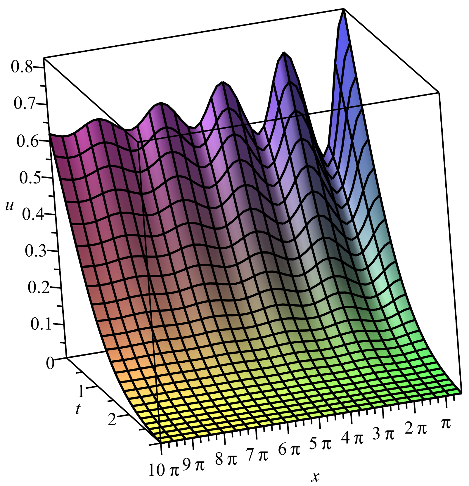
As a result, a similar theorem to Theorem 9 can be formulated; however, in this case, domain $\Omega$ can be also bounded (with a correctly-specified size) with respect to the variable x. Notably, the corresponding exact solution is periodic if $\lambda =0$ (i.e., the equation does not contain the convective term), and an example of such a solution is presented in Figure 1. In the case $\lambda \ne 0$, the solution is quasi-periodic, and the example is pictured in Figure 2. One also sees that Solution (120) with $\lambda >0$ is vanishing if $t\to +\infty$, and this means population extinction. The case $\lambda <0$ is similar to $\lambda >0$.

7. Conclusions

In this review, all the known results about Lie and Q-conditional (nonclassical) symmetries of the class of RDC equations with exponential nonlinearities (6) and their application for finding exact solutions are summarized. Many results about Lie symmetries and Lie’s (invariant) solutions of these equations have been known for a long time. However, we applied here two different approaches, the Lie–Ovsiannikov algorithm and the modern LSC algorithm based on FPTs, to the PDE class in question in order to show that all such equations with a non-trivial Lie symmetry are reducible just to two RDC equations (see Table 4). Moreover, a new theorem (see Theorem 3) is proven, which describes explicitly all FPTs for the PDE class (6), and examples of new exact solutions of some nonlinear RDC equations belonging to the above class are found.

In contrast to Lie’s symmetries, a vast majority of the Q-conditional symmetries presented here were derived very recently. As one may note, the structure of these symmetries is rather complicated (see Theorems 7 and 8). This notwithstanding, we were able to apply many Q-conditional symmetries to find exact solutions. The correctly-specified restrictions are found, which guarantee that they are non-Lie solutions. It was also shown that some of the exact solutions derived are obtainable via other modern techniques. Interestingly, the Q-conditional symmetry operator (102) with a cumbersome structure leads to the relatively simple non-Lie solution (107) of Equation (105), which seems to be new. We foresee that other symmetry operators presented in Theorem 8 can lead to new solutions of the nonlinear RDC Equation (59) and plan to report more new results in a forthcoming paper.

Many of the solutions obtained possess attractive properties and can be used for analytically solving the relevant boundary-value problems. In that particular case, exact solutions have been used to solve the boundary-value problem with the zero Neumann conditions for a generalization of the Fisher and Murray equations (see Theorem 9). As a result, a possible interpretation was presented for population dynamics. Moreover, the quasi-periodic solution was identified in order to demonstrate another scenario of the population evolution.

Finally, we present the following observation. The Q-conditional symmetry (57) with $a=0$ (see Case 2 of Table 6) takes the form:

$$Q={\partial }_t+(f(t)+{\lambda }_2{e}^{-u}){\partial }_u.$$

(121)

The first-order prolongation of this operator is:

$$\underset{1}{Q}={\partial }_t+(f(t)+{\lambda }_2{e}^{-u}){\partial }_u-{\lambda }_2{e}^{-u}{u}_x{\partial }_{u_x}-(f^{\prime }(t)-{\lambda }_2{e}^{-u}{u}_t){\partial }_{u_t}.$$

(122)

Consider the boundary-value problem in the domain $\Omega =\{(t,x)\in (0,+\infty )\times (A,B)\}$ (A and B are constants) consisting of Equation (56) and the zero flux conditions:

$$u_x(t,A)=0,u_x(t,B)=0.$$

(123)

Using Definition 2 [52], one can easily check that this nonlinear boundary-value problem (not its governing equation only!) admits the Q-conditional symmetry (121). Therefore, we foresee that exact solutions can be derived for such a kind of problem.