Lie Symmetries of Nonlinear Parabolic-Elliptic Systems and Their Application to a Tumour Growth Model

Abstract

A generalisation of the Lie symmetry method is applied to classify a coupled system of reaction-diffusion equations wherein the nonlinearities involve arbitrary functions in the limit case in which one equation of the pair is quasi-steady but the other is not. A complete Lie symmetry classification, including a number of the cases characterised as being unlikely to be identified purely by intuition, is obtained. Notably, in addition to the symmetry analysis of the PDEs themselves, the approach is extended to allow the derivation of exact solutions to specific moving-boundary problems motivated by biological applications (tumour growth). Graphical representations of the solutions are provided and a biological interpretation is briefly addressed. The results are generalised on multi-dimensional case under the assumption of the radially symmetrical shape of the tumour.

1. Introduction

It is well-known that nonlinear reaction-diffusion (RD) systems (i.e., systems of second-order parabolic PDEs with reaction terms) are used to describe various processes in physics, chemistry, biology, ecology, etc. (see, e.g., books [1,2,3,4]). Indeed, there are many special cases of such systems describing real world processes, among the most famous being Lotka–Volterra type systems [5,6] and systems used for modelling the chemical basis of morphogenesis [7] (see, e.g., ref. [2] for details in modern terminology).

The most common are two-component RD systems of the form

$$\begin{array}{c}{U}_t={\left(D_1\left(U\right)U_x\right)}_x+F(U,V),\hfill \\ V_t={\left(D_2\left(V\right)V_x\right)}_x+G(U,V),\hfill \end{array}$$

(1)

where $U(t,x)$ and $V(t,x)$ are unknown functions, the nonnegative smooth functions $D_1\left(U\right)$ and $D_2\left(V\right)$ are coefficients of diffusivity (conductivity), and F and G are arbitrary smooth functions describing the interaction between components $U(t,x)$ and $V(t,x)$. Hereafter the t and x subscripts denote differentiation with respect to these variables.

It should be noted that the search of Lie symmetries of RD systems was initiated many years ago and probably paper [8] was the first in this direction. A complete Lie symmetry classification was done much later because this problem is much more complicated in comparison with the case of a single RD equation. In particular, it was necessary to treat separately the cases of constant diffusivities (i.e., semilinear equations) and nonconstant (quasilinear) ones. All possible Lie symmetries of (1) with constant diffusivities were completely described in [9,10,11]. In the case of nonconstant diffusivities, it has been done in [12,13] (in [14], the result was extended to the multi-component RD systems).

It should be stressed that there are models used to describe real world processes that are based on singular limits of a RD system (1), namely with $D_2\left(V\right)=0$ or with the $V_t$ term absent. The system (1) with $D_2\left(V\right)=0$ has been used to describe interactions involving species (cells) V, which are not able to diffuse in space (typical examples include some models for plankton). Some particular results about Lie symmetries of such systems have been recently obtained in [15], however the problem of a complete Lie symmetry classification is still not solved.

Here, however, we examine the class of systems (1) with the $V_t$ term negligible so that V is governed by a quasi-steady equation, i.e.,

$$\begin{array}{c}{U}_t={\left(D_1\left(U\right)U_x\right)}_x+F(U,V),\hfill \\ 0={\left(D_2\left(V\right)V_x\right)}_x+G(U,V).\hfill \end{array}$$

(2)

Obviously this system is reduced to the form

$$\begin{array}{c}{U}_t={\left(D_1\left(U\right)U_x\right)}_x+F^{*}(U,V^{*}),\hfill \\ 0=V_{xx}^{*}+G^{*}(U,V^{*})\hfill \end{array}$$

(3)

by the Kirchhoff substitution for the component $V\to V^{*}$. Here the diffusivity $D_1\left(U\right)$ is a nonnegative and nonconstant function (at least in some domains) in what follows. We remind the reader that the case $D_1\left(U\right)=const$ was studied in [9,10]. Thus, the class of parabolic-elliptic systems (3) with $D_1\left(U\right)\ne const$ is the main object of this study. The main motivation for this follows from paper [16], in which a model for tumour growth was derived. Under some biologically motivated assumptions (see p. 570 in [16] for details), the model was simplified to a boundary-value problem with governing equations of the form (3). System (2) is of course potentially of relevance to any two-component RD model in which one species diffuses much faster than the other; it is also of interest purely from the symmetry point of view, since its symmetries differ essentially from those of (1).

The paper is organized as follows. Section 2 is devoted to the search for form-preserving transformations for the class of systems (3) in order to establish possible relations between RD systems that admit equivalent Lie symmetry algebras. Section 3 is devoted to the identification of all possible Lie symmetries that any system of the form (3) can admit. The main results of this section are presented in the form of

Table 1. Lie symmetries of system (4) in the case $F_V{G}_U\ne 0$.

Case	RD System	Basic Operators of MAI
1.	$U_t={\left(D\left(U\right)U_x\right)}_x+e^{V}f\left(U\right)$	${\partial }_t,{\partial }_x,2t{\partial }_t+x{\partial }_x-2{\partial }_V$
	$0=V_{xx}+e^{V}g\left(U\right)$
2.	$U_t={\left(D\left(U\right)U_x\right)}_x+V^{\beta }f\left(U\right)$	${\partial }_t,{\partial }_x,2\beta t{\partial }_t+\beta x{\partial }_x-2V{\partial }_V$
	$0=V_{xx}+V^{\beta +1}g\left(U\right)$
3.	$U_t={\left(U^k{U}_x\right)}_x+U^{\gamma +1}f\left(e^V{U}^{\alpha }\right)$	${\partial }_t,{\partial }_x,$
	$0=V_{xx}+U^{\gamma -k}g\left(e^V{U}^{\alpha }\right)$	$2\gamma t{\partial }_t+(\gamma -k)x{\partial }_x-2U{\partial }_U+2\alpha {\partial }_V$
4.	$U_t={\left(U^k{U}_x\right)}_x+U^{\gamma +1}f\left(V{U}^{\beta }\right)$	${\partial }_t,{\partial }_x,$
	$0=V_{xx}+V{U}^{\gamma -k}g\left(V{U}^{\beta }\right)$	$2\gamma t{\partial }_t+(\gamma -k)x{\partial }_x-2U{\partial }_U+2\beta V{\partial }_V$
5.	$U_t={\left(U^k{U}_x\right)}_x+{\alpha }_1{e}^V{U}^{\gamma +1}$	${\partial }_t,{\partial }_x,2t{\partial }_t+x{\partial }_x-2{\partial }_V,$
	$0=V_{xx}+{\alpha }_2{e}^V{U}^{\gamma -k}$	$kt{\partial }_t-U{\partial }_U+(\gamma -k){\partial }_V$
6.	$U_t={\left(U^k{U}_x\right)}_x+{\alpha }_1{V}^{\beta }{U}^{\gamma +1}$	${\partial }_t,{\partial }_x,2\beta t{\partial }_t+\beta x{\partial }_x-2V{\partial }_V,$
	$0=V_{xx}+{\alpha }_2{V}^{\beta +1}{U}^{\gamma -k}$	$k\beta t{\partial }_t-\beta U{\partial }_U+(\gamma -k)V{\partial }_V$
7.	$U_t={\left(U^k{U}_x\right)}_x+{\alpha }_1{U}^{k+1}+UV$	${\partial }_t,{\partial }_x,-k\phi \left(t\right){\partial }_t+\dot{\phi }\left(t\right)U{\partial }_U+$
	$0=V_{xx}+{\alpha }_2{U}^k$	$\left(k\dot{\phi }\left(t\right)V+(k+1)\ddot{\phi }\left(t\right)\right){\partial }_V$
8.	$U_t={\left(U^{-4/3}{U}_x\right)}_x+Uf\left(U{V}^3\right)$	${\partial }_t,{\partial }_x,2x{\partial }_x-3U{\partial }_U+V{\partial }_V,$
	$0=V_{xx}+Ug\left(U{V}^3\right)$	$x^2{\partial }_x-3xU{\partial }_U+xV{\partial }_V$
9.	$U_t={\left(U^{-4/3}{U}_x\right)}_x+{\alpha }_1{U}^{1+\gamma }{V}^{3\gamma }$	${\partial }_t,{\partial }_x,2x{\partial }_x-3U{\partial }_U+V{\partial }_V,$
	$0=V_{xx}+{\alpha }_2{U}^{4/3+\gamma }{V}^{3\gamma +1}$	$x^2{\partial }_x-3xU{\partial }_U+xV{\partial }_V,$
		$4\gamma t{\partial }_t+3\gamma U{\partial }_U-(4/3+\gamma )V{\partial }_V$
10.	$U_t={\left(e^U{U}_x\right)}_x+e^{(\gamma +1)U}f\left(V+\alpha U\right)$	${\partial }_t,{\partial }_x,$
	$0=V_{xx}+e^{\gamma U}g\left(V+\alpha U\right)$	$2(\gamma +1)t{\partial }_t+\gamma x{\partial }_x-2{\partial }_U+2\alpha {\partial }_V$
11.	$U_t={\left(e^U{U}_x\right)}_x+e^{(\gamma +1)U}f\left(V{e}^{\beta U}\right)$	${\partial }_t,{\partial }_x,$
	$0=V_{xx}+V{e}^{\gamma U}g\left(V{e}^{\beta U}\right)$	$2(\gamma +1)t{\partial }_t+\gamma x{\partial }_x-2{\partial }_U+2\beta V{\partial }_V$
12.	$U_t={\left(e^U{U}_x\right)}_x+{\alpha }_{1}exp\left((\gamma +1)U+V\right)$	${\partial }_t,{\partial }_x,2t{\partial }_t+x{\partial }_x-2{\partial }_V,$
	$0=V_{xx}+{\alpha }_{2}exp\left(\gamma U+V\right)$	$t{\partial }_t-{\partial }_U+\gamma {\partial }_V$
13.	$U_t={\left(e^U{U}_x\right)}_x+{\alpha }_1{e}^{(\gamma +1)U}{V}^{\beta }$	${\partial }_t,{\partial }_x,2\beta t{\partial }_t+\beta x{\partial }_x-2V{\partial }_V,$
	$0=V_{xx}+{\alpha }_2{e}^{\gamma U}{V}^{\beta +1}$	$\beta t{\partial }_t-\beta {\partial }_U+\gamma V{\partial }_V$
14.	$U_t={\left(e^U{U}_x\right)}_x+{\alpha }_1{e}^U+V$	${\partial }_x,\phi \left(t\right){\partial }_t-\dot{\phi }\left(t\right){\partial }_U-$
	$0=V_{xx}+{\alpha }_2{e}^U$	$\left(\dot{\phi }\left(t\right)V+\ddot{\phi }\left(t\right)\right){\partial }_V$

and

Table 2. Lie symmetries of system (4) in the case $F_V{G}_U=0$ and ${\left(F_V\right)}^2+{\left(G_U\right)}^2\ne 0$.

Case	RD System	Basic Operators of MAI
1.	$U_t={\left(D\left(U\right)U_x\right)}_x$	${\partial }_t,{\partial }_x,2t{\partial }_t+x{\partial }_x+2V{\partial }_V,$
	$0=V_{xx}+g\left(U\right)$	$\phi \left(t\right)x{\partial }_V,\psi \left(t\right){\partial }_V$
2.	$U_t={\left(D\left(U\right)U_x\right)}_x+f\left(U\right)$	${\partial }_t,{\partial }_x,\psi \left(t\right)V{\partial }_V$
	$0=V_{xx}+Vg\left(U\right)$
3.	$U_t={\left(D\left(U\right)U_x\right)}_x+f\left(U\right)$	${\partial }_t,{\partial }_x,h(t,x){\partial }_V$
	$0=V_{xx}+{\alpha }_{2}V+g\left(U\right)$
4.	$U_t={\left(U^k{U}_x\right)}_x+{\alpha }_0{U}^{\beta +1}$	${\partial }_t,{\partial }_x,2\beta t{\partial }_t+(\beta -k)x{\partial }_x-2U{\partial }_U,$
	$0=V_{xx}+\alpha V{U}^{\beta -k},\alpha \ne 0$	$\psi \left(t\right)V{\partial }_V$
5.	$U_t={\left(U^k{U}_x\right)}_x+UV$	${\partial }_x,kx{\partial }_x+2U{\partial }_U,-k\phi \left(t\right){\partial }_t+$
	$0=V_{xx}$	$\dot{\phi }\left(t\right)U{\partial }_U+(k\dot{\phi }\left(t\right)V+(k+1)\ddot{\phi }\left(t\right)){\partial }_V$
6.	$U_t={\left(U^k{U}_x\right)}_x+{\alpha }_1{U}^{k+1}$	${\partial }_t,{\partial }_x,-kt{\partial }_t+U{\partial }_U+h^0\left(x\right){\partial }_V,h(t,x){\partial }_V,$
	$0=V_{xx}+lnU+{\alpha }_{2}V$
7.	$U_t={\left(U^k{U}_x\right)}_x+{\alpha }_1{U}^{k+1}$	${\partial }_t,{\partial }_x,-kt{\partial }_t+U{\partial }_U+\beta V{\partial }_V,$
	$0=V_{xx}+U^{\beta }+{\alpha }_{2}V$	$h(t,x){\partial }_V$
8.	$U_t={\left(U^k{U}_x\right)}_x+\alpha U^{\gamma +1},\alpha \gamma \ne 0$	${\partial }_t,{\partial }_x,2\gamma t{\partial }_t+(\gamma -k)x{\partial }_x-2U{\partial }_U+$
	$0=V_{xx}+lnU$	$\left(2(\gamma -k)V+x^2\right){\partial }_V,\phi \left(t\right)x{\partial }_V,\psi \left(t\right){\partial }_V$
9.	$U_t={\left(U^k{U}_x\right)}_x+\alpha U^{\gamma +1},\alpha \gamma \ne 0$	${\partial }_t,{\partial }_x,2\gamma t{\partial }_t+(\gamma -k)x{\partial }_x-2U{\partial }_U+$
	$0=V_{xx}+U^{\beta }$	$2(\gamma -\beta -k)V{\partial }_V,\phi \left(t\right)x{\partial }_V,\psi \left(t\right){\partial }_V$
10.	$U_t={\left(U^k{U}_x\right)}_x$	${\partial }_t,{\partial }_x,-2kt{\partial }_t+2U{\partial }_U-x^2{\partial }_V,$
	$0=V_{xx}+lnU$	$2t{\partial }_t+x{\partial }_x+2V{\partial }_V,\phi \left(t\right)x{\partial }_V,\psi \left(t\right){\partial }_V$
11.	$U_t={\left(U^k{U}_x\right)}_x$	${\partial }_t,{\partial }_x,-kt{\partial }_t+U{\partial }_U+\beta V{\partial }_V,$
	$0=V_{xx}+U^{\beta }$	$2t{\partial }_t+x{\partial }_x+2V{\partial }_V,\phi \left(t\right)x{\partial }_V,\psi \left(t\right){\partial }_V$
12.	$U_t={\left(U^{-4/3}{U}_x\right)}_x+\alpha U,\alpha \ne 0$	${\partial }_t,{\partial }_x,2x{\partial }_x-3U{\partial }_U+V{\partial }_V,\phi \left(t\right)x{\partial }_V$
	$0=V_{xx}+U$	$x^2{\partial }_x-3xU{\partial }_U+xV{\partial }_V,\psi \left(t\right){\partial }_V$
13.	$U_t={\left(U^{-4/3}{U}_x\right)}_x$	${\partial }_t,{\partial }_x,2x{\partial }_x-3U{\partial }_U+V{\partial }_V,$
	$0=V_{xx}+U$	$x^2{\partial }_x-3xU{\partial }_U+xV{\partial }_V,$
		$4t{\partial }_t+3\left(U{\partial }_U+V{\partial }_V\right),\phi \left(t\right)x{\partial }_V,\psi \left(t\right){\partial }_V$
14.	$U_t={\left(e^U{U}_x\right)}_x+{\alpha }_0{e}^{(\beta +1)U}$	${\partial }_t,{\partial }_x,2(\beta +1)t{\partial }_t+\beta x{\partial }_x-2{\partial }_U,$
	$0=V_{xx}+\alpha V{e}^{\beta U},\alpha \ne 0$	$\psi \left(t\right)V{\partial }_V$
15.	$U_t={\left(e^U{U}_x\right)}_x+V$	${\partial }_t,{\partial }_x,x{\partial }_x+2{\partial }_U,$
	$0=V_{xx}$	$\phi \left(t\right){\partial }_t-\dot{\phi }\left(t\right){\partial }_U-\left(\dot{\phi }\left(t\right)V+\ddot{\phi }\left(t\right)\right){\partial }_V$
16.	$U_t={\left(e^U{U}_x\right)}_x+{\alpha }_1{e}^U$	${\partial }_t,{\partial }_x,-t{\partial }_t+{\partial }_U+h^0\left(x\right){\partial }_V,h(t,x){\partial }_V$
	$0=V_{xx}+U+{\alpha }_{2}V$
17.	$U_t={\left(e^U{U}_x\right)}_x+{\alpha }_1{e}^U$	${\partial }_t,{\partial }_x,-t{\partial }_t+{\partial }_U+\beta V{\partial }_V,h(t,x){\partial }_V$
	$0=V_{xx}+e^{\beta U}+{\alpha }_{2}V$
18.	$U_t={\left(e^U{U}_x\right)}_x+\alpha e^{\gamma U},\alpha \gamma \ne 0$	${\partial }_t,{\partial }_x,2\gamma t{\partial }_t+(\gamma -1)x{\partial }_x-2{\partial }_U+$
	$0=V_{xx}+U$	$\left(2(\gamma -1)V+x^2\right){\partial }_V,\phi \left(t\right)x{\partial }_V,\psi \left(t\right){\partial }_V$
19.	$U_t={\left(e^U{U}_x\right)}_x+\alpha e^{\gamma U},\alpha \gamma \ne 0$	${\partial }_t,{\partial }_x,2\gamma t{\partial }_t+(\gamma -1)x{\partial }_x-2{\partial }_U+$
	$0=V_{xx}+e^{\beta U}$	$2(\gamma -\beta -1)V{\partial }_V,\phi \left(t\right)x{\partial }_V,\psi \left(t\right){\partial }_V$
20.	$U_t={\left(e^U{U}_x\right)}_x$	${\partial }_t,{\partial }_x,2t{\partial }_t-2{\partial }_U+x^2{\partial }_V,$
	$0=V_{xx}+U$	$2t{\partial }_t+x{\partial }_x+2V{\partial }_V,\phi \left(t\right)x{\partial }_V,\psi \left(t\right){\partial }_V$
21.	$U_t={\left(e^U{U}_x\right)}_x$	${\partial }_t,{\partial }_x,t{\partial }_t-{\partial }_U-\beta V{\partial }_V,$
	$0=V_{xx}+e^{\beta U}$	$2t{\partial }_t+x{\partial }_x+2V{\partial }_V,\phi \left(t\right)x{\partial }_V,\psi \left(t\right){\partial }_V$

. In Section 4 and Section 5, we apply the Lie symmetries derived for the reduction of a nonlinear boundary value problem (BVP) with a free boundary modeling tumour growth in order to construct its exact solution. Moreover, possible biological interpretations of the results derived are discussed. Finally, we briefly discuss the result obtained and present some conclusions in the last section.

2. Form-Preserving Transformations for the Class of Systems (3)

First of all we simplify notations in system (3) in a natural way:

$$\begin{array}{c}{U}_t={\left(D\left(U\right)U_x\right)}_x+F(U,V),\hfill \\ 0=V_{xx}+G(U,V).\hfill \end{array}$$

(4)

The class of systems (4) contains three arbitrary functions and the Lie symmetry of its different representatives depends essentially on the form of the triplet $(D,F,G)$. Thus, the problem of a complete description of all possible Lie symmetries (the so called group classification problem) arises. In order to solve this, we can apply the Lie–Ovsiannikov approach (the name of Ovsiannikov arises because he published a remarkable paper in this direction, [17]) of the Lie symmetry classification, which is based on the classical Lie scheme and a set of equivalence transformations of the differential equation in question. However, it is well-known that this approach leads to a very long list of equations with nontrivial Lie symmetry provided the given equation (system) contains several arbitrary functions (system (4) involves three such).

During the last two decades, new approaches for solving group classification problems were developed, which are important for obtaining the so called canonical list of inequivalent equations admitting nontrivial Lie symmetry algebras and allowing the solution of this problem in a more efficient way than a formal application of the Lie–Ovsiannikov approach. Here we use the algorithm based on so called form-preserving transformations [18,19], which were used initially for finding locally-equivalent PDEs, especially those nonlinear PDEs that are linearizable by a point transformation. Interestingly, such transformations were implicitly used much earlier in [20] in order to find all possible heat equations with nonlinear sources that admit the Lie symmetry either of the linear heat equation or the Burgers equation. In [21], these transformations are called ‘allowed transformations’ and they were used to classify the Lie symmetries of a class of variable coefficient Korteweg-de Vries equations. One may say that the above cited paper was the first one, in which allowed (form-preserving) transformations were systematically used for solving the Lie symmetry classification problem. Now we present the definition of form-preserving transformations in the case of the class of systems (4).

Definition 1.

A point non-degenerate transformation given by the formulae

$$\begin{array}{c}t=a(\tau ,y,u,v),x=b(\tau ,y,u,v),\hfill \\ U=\phi (\tau ,y,u,v),V=\psi (\tau ,y,u,v),\hfill \end{array}$$

(5)

which maps at least one system of the form (4) into a system belonging to the same class, is called a form-preserving transformation.

Comparing this definition with the well-known definition for equivalence transformations, one immediately notes that each equivalence transformation is automatically a form-preserving transformation, but not vice versa.

It was noted later [22,23] that the form-preserving transformations (nowadays the terminology ‘admissible transformations’ is also widely used) allow an essential reduction of the number of cases obtained via the classical Lie–Ovsiannikov algorithm (see extensive discussions on this matter in [11,13,24]). In particular, it is shown in [13] that there are only 10 inequivalent cases when RD systems with nonconstant diffusivities and reaction terms of the form (1) are invariant with respect to the nontrivial Lie algebras (in contrast to a much longer list derived in [12] via the Lie–Ovsiannikov algorithm). Similarly, it was proved in [24] that the canonical list of inequivalent reaction-diffusion-convection equations consists of 15 equations only (not the 30 derived by the Lie–Ovsiannikov algorithm).

The reader may find more details (including specific examples) on this matter in Section 2.3 of the recent book [25].

Now we present the main result of this section, namely the theorem describing a general form of form-preserving transformations for the class of systems (4).

Theorem 1.

An arbitrary system of the form

$$\begin{array}{c}{u}_{\tau }={\left(\tilde{D}\left(u\right)u_y\right)}_y+\tilde{F}(u,v),\hfill \\ 0=v_{yy}+\tilde{G}(u,v)\hfill \end{array}$$

(6)

can be reduced to a system from class (4) by a form-preserving transformation of the form (5) if and only if the smooth functions $a,b,\phi$ and ψ have the forms

$$\begin{array}{c}a=\alpha \left(\tau \right),b=\beta (\tau ,y),{\alpha }_{\tau }{\beta }_y\ne 0,\hfill \\ \phi =K(\tau ,y)u+P(\tau ,y),K\ne 0,\hfill \\ \psi =L(\tau ,y)v+Q(\tau ,y),L\ne 0,\hfill \end{array}$$

(7)

where the functions $\alpha \left(\tau \right),\beta (\tau ,y),K(\tau ,y),P(\tau ,y),L(\tau ,y)$ and $Q(\tau ,y)$ are such that the following equalities

$$\begin{array}{c}{\alpha }_{\tau }D={\beta }_y^2\tilde{D},\hfill \\ {\alpha }_{\tau }F=K\tilde{F}+\frac{{(K_{y}u+P_y)}^2}{K}{\tilde{D}}_u+K_{\tau }u+P_{\tau }-\tilde{D}\left(K_{yy}u+P_{yy}-2\frac{K_{y}u+P_y}{K}{K}_y\right),\hfill \\ {\beta }_y^{2}G=L\tilde{G}+2\frac{L_{y}v+Q_y}{L}{L}_y-L_{yy}v-Q_{yy},\hfill \\ 2{\beta }_y(K_{y}u+P_y){\tilde{D}}_u+\tilde{D}\left(2{\beta }_y{K}_y-{\beta }_{yy}K\right)+{\beta }_{\tau }K=0,\hfill \\ 2{\beta }_y{L}_y-{\beta }_{yy}L=0,\hfill \end{array}$$

(8)

hold.

The proof of Theorem 1

is quite similar to that for the class of RD systems (1) with $D_k=const(k=1,2)$ presented in [26].

The group of equivalence transformations can be easily extracted from Theorem 1 by assuming that $\tilde{D},\tilde{F}$ and $\tilde{G}$ are arbitrary smooth functions. Solving the system (8) under such condition one arrives at the following statement. ☐

Consequence 1.

The group of equivalence transformations for (4) has the form

$$\begin{array}{c}t={\alpha }_1\tau +{\alpha }_2,x={\alpha }_{3}y+{\alpha }_4,\hfill \\ U={\alpha }_{5}u+{\alpha }_6,V={\alpha }_{7}v+{\alpha }_8,\hfill \\ D=\frac{{\alpha }_3^2}{{\alpha }_1}\tilde{D},F=\frac{{\alpha }_5}{{\alpha }_1}\tilde{F},G=\frac{{\alpha }_7}{{\alpha }_3^2}\tilde{G},\hfill \end{array}$$

(9)

where ${\alpha }_l(l=1,\dots ,8)$ are arbitrary group parameters (${\alpha }_1>0,{\alpha }_{2k-1}\ne 0,k=2,3,4$).

One sees that (8) is a nonlinear system of functional-differential equations and its general solution seems to be impossible without further restrictions. For example, assuming a constant diffusivity $\tilde{D}$, one may derive that $\beta (\tau ,y)$ is linear with respect to (w.r.t.) the variable y; however, $\beta (\tau ,y)$ can be nonlinear for the nonconstant diffusivity $\tilde{D}$ (see

Table 3. RD systems that are reduced to those in Table 1 by the form-preserving transformations.

	RD System	Transformation of Variables	Case of Table 1
1.	$u_{\tau }={\left(u^k{u}_y\right)}_y+u^{k+1}f\left(e^v{u}^{\alpha }\right)+\lambda u$	$U=e^{-\lambda \tau }u,V=v+\alpha \lambda \tau ,$	3
	$0=v_{yy}+g\left(e^v{u}^{\alpha }\right)$	$t=\frac{1}{k\lambda }{e}^{k\lambda \tau }$	with $\gamma =k$
2.	$u_{\tau }={\left(u^k{u}_y\right)}_y+u^{k+1}f\left(v{u}^{\beta }\right)+\lambda u$	$U=e^{-\lambda \tau }u,V=e^{\beta \lambda \tau }v,$	4
	$0=v_{yy}+vg\left(v{u}^{\alpha }\right)$	$t=\frac{1}{k\lambda }{e}^{k\lambda \tau }$	with $\gamma =k$
3.	$u_{\tau }={\left(u^{-4/3}{u}_y\right)}_y+uf\left(u{v}^3\right)-3u^{-1/3}$	$U=u{cos}^{3}y,V=v{cos}^{-1}y,$	8
	$0=v_{yy}+ug\left(u{v}^3\right)+v$	$x=tany$
4.	$u_{\tau }={\left(u^{-4/3}{u}_y\right)}_y+uf\left(u{v}^3\right)+3u^{-1/3}$	$U=e^{3y}u,V=e^{-y}v,$	8
	$0=v_{yy}+ug\left(u{v}^3\right)-v$	$x=\frac{1}{2}{e}^{-2y}$
5.	$u_{\tau }={\left(u^{-4/3}{u}_y\right)}_y+{\alpha }_1{u}^{1+\gamma }{v}^{3\gamma }-3u^{-1/3}$	$U=u{cos}^{3}y,V=v{cos}^{-1}y,$	9
	$0=v_{yy}+{\alpha }_2{u}^{4/3+\gamma }{v}^{3\gamma +1}+v$	$x=tany$
6.	$u_{\tau }={\left(u^{-4/3}{u}_y\right)}_y+{\alpha }_1{u}^{1+\gamma }{v}^{3\gamma }+3u^{-1/3}$	$U=e^{3y}u,V=e^{-y}v,$	9
	$0=v_{yy}+{\alpha }_2{u}^{4/3+\gamma }{v}^{3\gamma +1}-v$	$x=\frac{1}{2}{e}^{-2y}$
7.	$u_{\tau }={\left(e^u{u}_y\right)}_y+e^{u}f\left(v+\alpha u\right)+\lambda$	$U=u-\lambda \tau ,V=v+\alpha \lambda \tau ,$	10
	$0=v_{yy}+g\left(v+\alpha u\right)$	$t=\frac{1}{\lambda }{e}^{\lambda \tau }$	with $\gamma =0$
8.	$u_{\tau }={\left(e^u{u}_y\right)}_y+e^{u}f\left(v{e}^{\beta u}\right)+\lambda$	$U=u-\lambda \tau ,V=e^{\beta \lambda \tau }v,$	11
	$0=v_{yy}+vg\left(v{e}^{\beta u}\right)$	$t=\frac{1}{\lambda }{e}^{\lambda \tau }$	with $\gamma =0$

and

Table 4. RD systems that are reduced to those in Table 2 by the form-preserving transformations.

	RD System	Transformation of Variables	Case of Table 2
1.	$u_{\tau }={\left(u^k{u}_y\right)}_y+{\alpha }_1{u}^{k+1}+\lambda u$	$U=e^{-\lambda \tau }u,t=\frac{1}{k\lambda }{e}^{k\lambda \tau },$	6
	$0=v_{yy}+lnu+{\alpha }_{2}v$	$V=\left\{\begin{array}{cc}v+\frac{\lambda }{{\alpha }_2}\tau ,\hfill & if{\alpha }_2\ne 0,\hfill \\ v+\frac{\lambda }{2}\tau y^2,\hfill & if{\alpha }_2=0\hfill \end{array}\right.$
2.	$u_{\tau }={\left(u^k{u}_y\right)}_y+{\alpha }_1{u}^{k+1}+\lambda u$	$U=e^{-\lambda \tau }u,t=\frac{1}{k\lambda }{e}^{k\lambda \tau },$	7
	$0=v_{yy}+u^{\beta }+{\alpha }_{2}v+\gamma$	$V=\left\{\begin{array}{cc}\left(v+\frac{\gamma }{{\alpha }_2}\right)e^{-\beta \lambda \tau },\hfill & if{\alpha }_2\ne 0,\hfill \\ \left(v+\frac{\gamma }{2}{y}^2\right)e^{-\beta \lambda \tau },\hfill & if{\alpha }_2=0\hfill \end{array}\right.$
3.	$u_{\tau }={\left(u^k{u}_y\right)}_y+\alpha u^{\gamma +1}$	$V=v+\frac{\lambda }{2}{y}^2$	9, if $\alpha \ne 0$
	$0=v_{yy}+u^{\beta }+\lambda$		11, if $\alpha =0$
4.	$u_{\tau }={\left(u^k{u}_y\right)}_y+\lambda u$	$U=e^{-\lambda \tau }u,t=\frac{1}{k\lambda }{e}^{k\lambda \tau },$	10
	$0=v_{yy}+lnu$	$V=v+\frac{\lambda }{2}\tau y^2$
5.	$u_{\tau }={\left(u^k{u}_y\right)}_y+\lambda u$	$U=e^{-\lambda \tau }u,t=\frac{1}{k\lambda }{e}^{k\lambda \tau },$	11
	$0=v_{yy}+u^{\beta }+\gamma$	$V=\left(v+\frac{\gamma }{2}{y}^2\right)e^{-\beta \lambda \tau }$
6.	$u_{\tau }={\left(u^{-4/3}{u}_y\right)}_y+\alpha u-3u^{-1/3}$	$U=u{cos}^{3}y,V=v{cos}^{-1}y,$	12
	$0=v_{yy}+u+v$	$x=tany$
7.	$u_{\tau }={\left(u^{-4/3}{u}_y\right)}_y+\alpha u+3u^{-1/3}$	$U=e^{3y}u,V=e^{-y}v,$	12
	$0=v_{yy}+u-v$	$x=\frac{1}{2}{e}^{-2y}$
8.	$u_{\tau }={\left(u^{-4/3}{u}_y\right)}_y-3u^{-1/3}$	$U=u{cos}^{3}y,V=v{cos}^{-1}y,$	13
	$0=v_{yy}+u+v$	$x=tany$
9.	$u_{\tau }={\left(u^{-4/3}{u}_y\right)}_y+3u^{-1/3}$	$U=e^{3y}u,V=e^{-y}v,$	13
	$0=v_{yy}+u-v$	$x=\frac{1}{2}{e}^{-2y}$
10.	$u_{\tau }={\left(e^u{u}_y\right)}_y+{\alpha }_1{e}^u+\lambda$	$U=u-\lambda \tau ,t=\frac{1}{\lambda }{e}^{\lambda \tau },$	16
	$0=v_{yy}+u+{\alpha }_{2}v$	$V=\left\{\begin{array}{cc}v+\frac{\lambda }{{\alpha }_2}\tau ,\hfill & if{\alpha }_2\ne 0,\hfill \\ v+\frac{\lambda }{2}\tau y^2,\hfill & if{\alpha }_2=0\hfill \end{array}\right.$
11.	$u_{\tau }={\left(e^u{u}_y\right)}_y+{\alpha }_1{e}^u+\lambda$	$U=u-\lambda \tau ,t=\frac{1}{\lambda }{e}^{\lambda \tau },$	17
	$0=v_{yy}+e^{\beta u}+{\alpha }_{2}v+\gamma$	$V=\left\{\begin{array}{cc}\left(v+\frac{\gamma }{{\alpha }_2}\right)e^{-\beta \lambda \tau },\hfill & if{\alpha }_2\ne 0,\hfill \\ \left(v+\frac{\gamma }{2}{y}^2\right)e^{-\beta \lambda \tau },\hfill & if{\alpha }_2=0\hfill \end{array}\right.$
12.	$u_{\tau }={\left(e^u{u}_y\right)}_y+\alpha e^{\gamma u}$	$V=v+\frac{\lambda }{2}{y}^2$	19, if $\alpha \ne 0$
	$0=v_{yy}+e^{\beta u}+\lambda$		21, if $\alpha =0$
13.	$u_{\tau }={\left(e^u{u}_y\right)}_y+\lambda$	$U=u-\lambda \tau ,t=\frac{1}{\lambda }{e}^{\lambda \tau },$	20
	$0=v_{yy}+u$	$V=v+\frac{\lambda }{2}\tau y^2$
14.	$u_{\tau }={\left(e^u{u}_y\right)}_y+\lambda$	$U=u-\lambda \tau ,t=\frac{1}{\lambda }{e}^{\lambda \tau },$	21
	$0=v_{yy}+e^{\beta u}+\gamma$	$V=\left(v+\frac{\gamma }{2}{y}^2\right)e^{-\beta \lambda \tau }$

below for examples).

While the form of the transformations (7) is still quite general, it will be shown in the next section that only particular cases play important roles in solving the Lie symmetry classification problem for the nonlinear parabolic-elliptic systems (3).

3. Lie Symmetries of a Class of Parabolic-Elliptic Systems

In order to find Lie symmetry operators of a system of the form (4) via the Lie method [25,27,28,29,30,31], one needs to consider the manifold $(S_1,S_2)$

$$\begin{array}{c}{S}_1\equiv U_t-{\left(D\left(U\right)U_x\right)}_x-F(U,V)=0,\hfill \\ S_2\equiv V_{xx}+G(U,V)=0\hfill \end{array}$$

(10)

in the space of the following variables:

$$t,x,U,V,U_t,U_x,V_t,V_x,U_{tx},U_{tt},U_{xx},V_{tx},V_{tt},V_{xx}.$$

The system (4) is invariant under the transformations generated by the infinitesimal operator

$$X={\xi }^0(t,x,U,V){\partial }_t+{\xi }^1(t,x,U,V){\partial }_x+{\eta }^1(t,x,U,V){\partial }_U+{\eta }^2(t,x,U,V){\partial }_V$$

(11)

when the following invariance conditions are satisfied:

$$\begin{array}{c}\underset{2}{X}\left(S_1\right)\equiv \underset{2}{X}\left(U_t-{\left(D\left(U\right)U_x\right)}_x-F(U,V)\right){|}_{S_1=0,S_2=0}=0,\hfill \\ \underset{2}{X}\left(S_2\right)\equiv \underset{2}{X}\left(V_{xx}+G(U,V)\right){|}_{S_1=0,S_2=0}=0.\hfill \end{array}$$

(12)

The operator $\underset{2}{X}$ is the second prolongation of the operator X, i.e.,

$$\begin{array}{c}\underset{2}{X}=X+{\rho }_t^1\frac{\partial }{\partial U_t}+{\rho }_t^1\frac{\partial }{\partial V_t}+{\rho }_x^1\frac{\partial }{\partial U_x}+{\rho }_x^2\frac{\partial }{\partial V_x}+\hfill \\ {\sigma }_{tt}^1\frac{\partial }{\partial U_{tt}}+{\sigma }_{tx}^1\frac{\partial }{\partial U_{tx}}+{\sigma }_{xx}^1\frac{\partial }{\partial U_{xx}}+{\sigma }_{tt}^2\frac{\partial }{\partial V_{tt}}+{\sigma }_{tx}^2\frac{\partial }{\partial V_{tx}}+{\sigma }_{xx}^2\frac{\partial }{\partial V_{xx}},\hfill \end{array}$$

(13)

where the coefficients $\rho$ and $\sigma$ with relevant subscripts are calculated by well-known formulae (see, e.g., [29,30,31]).

Substituting (13) into (12) and eliminating the derivatives $U_t$ and $V_{xx}$ using (4), we can obtain the following system of determining equations (DEs):

$$\begin{array}{c}{\xi }_x^0={\xi }_U^0={\xi }_V^0={\xi }_U^1={\xi }_V^1=0,\hfill \end{array}$$

(14)

$$\begin{array}{c}{\eta }_V^1={\eta }_U^2={\eta }_{VV}^2=0,\hfill \end{array}$$

(15)

$$\begin{array}{c}\left(2{\xi }_x^1-{\xi }_t^0\right)D={\eta }^1{D}_U,\hfill \end{array}$$

(16)

$$\begin{array}{c}2{\eta }_{xV}^2={\xi }_{xx}^1,\hfill \end{array}$$

(17)

$$\begin{array}{c}\left({\xi }_{xx}^1-2{\eta }_{xU}^1\right)D=2{\eta }_x^1{D}_U+{\xi }_t^1,\hfill \end{array}$$

(18)

$$\begin{array}{c}\left(2{\xi }_x^1-{\xi }_t^0-{\eta }_U^1\right)D_U={\eta }_{UU}^{1}D+{\eta }^1{D}_{UU},\hfill \end{array}$$

(19)

$$\begin{array}{c}{\eta }^1{F}_U+{\eta }^2{F}_V={\eta }_t^1-D{\eta }_{xx}^1+F\left({\eta }_U^1-{\xi }_t^0\right),\hfill \end{array}$$

(20)

$$\begin{array}{c}{\eta }^1{G}_U+{\eta }^2{G}_V=-{\eta }_{xx}^2+G\left({\eta }_V^2-2{\xi }_x^1\right).\hfill \end{array}$$

(21)

Obviously, the general solution of the above system of DEs essentially depends on the form of the triplet $(D,F,G)$. Thus, the problem of a complete description of all possible Lie symmetries (the so called group classification problem) arises.

First of all we find the so called trivial algebra (other terminology used for this algebra is the ‘principal algebra’ and the ‘kernel of maximal invariance algebras’) of the class in question, i.e., the maximal invariance algebra (MAI) admitted by each equation of the form (4). Under the natural assumption that $D,F$ and G are arbitrary smooth functions the above system of DEs can be easily solved and the two-dimensional Lie algebra generated by the basic operators

$$X_1={\partial }_t,X_2={\partial }_x$$

(22)

is obtained.

In order to solve the problem of Lie symmetry classification for system (4), i.e., to find all possible systems admitting three- and higher-dimensional MAI, we use the algorithm based on form-preserving transformations, which was briefly discussed in Section 2. Moreover, it will be shown below that, similarly to the case of standard nonlinear RD systems [13], such an approach is also more efficient for parabolic-elliptic systems (compared to the classical Lie–Ovsiannikov algorithm).

Let us formulate a theorem which gives complete information on the classical symmetry of the nonlinear system (4).

Theorem 2.

All possible maximal algebras of invariance (up to equivalent representations generated by transformations of the form (23)) of the system (4) for any fixed nonconstant function D and nonconstant function vectors $(F,G)$ are presented in Table 1 and Table 2. Any other system of the form (6) with nontrivial Lie symmetry is reduced by a local substitution of the form

$$\begin{array}{c}t=C_0\tau +C_{1}exp\left(C_2\tau \right),\hfill \\ x=C_{3}y+C_{4}exp\left(C_{5}y\right)+C_{6}tan\left(C_{7}y\right),\hfill \\ U=C_8+C_9\tau +C_{10}exp\left(C_{11}\tau \right)u+\hfill \\ C_{4}exp\left(C_{12}y\right)u+C_6{cos}^3\left(C_{13}y\right)u,\hfill \\ V=C_{14}+C_{15}\tau +C_{16}exp\left(C_{17}\tau \right)v+C_{4}exp\left(C_{12}y\right)v+\hfill \\ C_6{cos}^{-1}\left(C_{13}y\right)v+C_{18}\tau y^2+C_{19}exp\left(C_{20}\tau \right)y^2,\hfill \end{array}$$

(23)

to one of those given in Table 1 and Table 2 (the constants C with subscripts are determined by the form of the system in question, some of them necessarily being zero in any given case).

Remark 1.

Each case in Table 1 contains semi-coupled systems (i.e., those with $F_V{G}_U=0$) as special subcases. A system specified in such a way has the same MAI provided it is not listed in Table 2 as a special case. For example, the system arising in case 1 with an arbitrary function $f\left(U\right)$ and $g\left(U\right)=const$ is a semi-coupled system; however, this is not listed in Table 2, so that its MAI is still a 3-dimensional Lie algebra.

Remark 2.

In Table 1 and Table 2, $\alpha ,{\alpha }_0,{\alpha }_1,{\alpha }_2,\beta ,\gamma ,k$ are arbitrary constants obeying the restriction $k\beta ({\left({\alpha }_1\right)}^2+{\left({\alpha }_2\right)}^2)\ne 0$; $D,f,g,\phi$ and ψ are arbitrary smooth functions of the relevant arguments; the function $h(t,x)$ is the general solution of the equation $h_{xx}+{\alpha }_{2}h=0,$ while $h^0\left(x\right)=\left\{\begin{array}{c}-\frac{1}{{\alpha }_2},if{\alpha }_2\ne 0,\hfill \\ -\frac{x^2}{2},if{\alpha }_2=0.\hfill \end{array}\right.$

The sketch of the proof of Theorem 2

Consider the determining Equations (14)–(21) under the assumption $D_U\ne 0$ (we remind the reader that the case $D_U=0$ was examined in [9,10]). Obviously, Equations (14)–(17) can be easily solved and the formulae

$$\begin{array}{c}{\xi }^0=a\left(t\right),{\xi }^1=b(t,x),\hfill \\ {\eta }^1=(2b_x-\dot{a})D{D}_U^{-1},{\eta }^2=r(t,x)V+p(t,x),r_x=\frac{1}{2}{b}_{xx}\hfill \end{array}$$

(24)

are obtained (here $a,b,r$ and p are arbitrary smooth functions and the upper dot means the time derivative).

Now we can consider Equations (18)–(21) as classification equations to find the function D and the pairs of the functions $(F,G)$ for which the system (4) has a nontrivial Lie symmetry, i.e., its MAI is larger than the trivial algebra (22).

It follows from (18)–(19) that there is a special case $2b_x=a_t$ when the diffusivity D can be an arbitrary smooth function. Indeed, Equation (18) produces $b_t=b_{xx}=0$ provided D is an arbitrary function. Hence, one arrives at $b=b_{1}x+b_0,a=2b_{1}t+a_0$, so that the classification Equations (20) and (21) have the form:

$$\begin{array}{c}(rV+p)F_V=-2b_{1}F,\hfill \\ (rV+p)G_V+G\left(2b_1-r\right)=-p_{xx}.\hfill \end{array}$$

(25)

The general solution of (25) depends essentially on the functions r and p ($r^2+p^2\ne 0$, otherwise a trivial Lie symmetry is obtained). In order to derive a complete result, one needs to examine two subcases.

Let us consider the first subcase $r=0,p\ne 0,$ i.e., the first equation in (25) takes the form $p{F}_V=-2b_{1}F$. A simple analysis says that the general solution of (25) leads to the functions $F,G$ and coefficients (24), which produce the system and MAI arising in case 1 of Table 1 provided $b_1\ne 0$. If $b_1=0$ then case 3 of Table 2 is derived.

The second subcase $r\ne 0$ leads to case 2 of Table 1 and cases 1 and 2 of Table 2.

The condition $2b_x-a_t\ne 0$ is a generic inequality and produces all other cases listed in Table 1 and Table 2. Using this condition and (24), one easily solves the Equation (19) and obtains

$$D=\left\{\begin{array}{c}d{(U+C_1)}^k,\hfill \\ dexp\left(C_{2}U\right),\hfill \end{array}\right.$$

(26)

where $d\ne 0,C_1,C_2$ and $k\ne 0$ are arbitrary constants. Moreover, substituting (26) into (18), we obtain $b=b_{1}x+b_0,b_0,b_1\in \mathbb{R},$ unless

$$D=d{(U+C_1)}^{-4/3},b=b\left(x\right).$$

(27)

One notes that the system (4) with diffusivities (26) and (27) can be simplified to one with $d=1,C_1=0,C_2=1$ by the appropriate equivalence transformations from (9).

Now one needs to examine other determining equations separately with power law diffusivity, exponential diffusivity and the special power law coefficient $k=-4/3$. We present here only the last case, i.e., the power low diffusivity $D=U^{-4/3}$, which is the most complicated.

Let us consider system (4) with $D=U^{-4/3}.$ It turns out that we may assume that ${\xi }_{xx}^1\ne 0$ (otherwise only particular cases of (4) with $D=U^k$ will be derived). The classification Equations (20) and (21) for $D=U^{-4/3}$ take the form

$$\begin{array}{c}\frac{3}{4}\left(\dot{a}-2b^{\prime }\right)U{F}_U+(rV+p)F_V+\left(\frac{\dot{a}}{4}+\frac{3b^{\prime }}{2}\right)F=\frac{3}{4}\ddot{a}U+\frac{3b^{\left(3\right)}}{2}{U}^{-1/3},\hfill \end{array}$$

(28)

$$\begin{array}{c}\frac{3}{4}\left(\dot{a}-2b^{\prime }\right)U{G}_U+(rV+p)G_V+\left(2b^{\prime }-r\right)G=-\frac{b^{\left(3\right)}}{2}V-p_{xx}.\hfill \end{array}$$

(29)

(because the function b depends only on x we use the standard notations for its derivatives and $b^{\left(k\right)}=\frac{d^{k}b}{d{x}^k},k=3,4\dots$). Now we construct differential consequences of (28) and (29) w.r.t. x:

$$\begin{array}{c}-\frac{3b^{″}}{2}U{F}_U+\left(\frac{b^{″}}{2}V+p_x\right)F_V+\frac{3b^{″}}{2}F=\frac{3b^{\left(4\right)}}{2}{U}^{-1/3},\hfill \end{array}$$

(30)

$$\begin{array}{c}-\frac{3b^{″}}{2}U{G}_U+\left(\frac{b^{″}}{2}V+p_x\right)G_V+\frac{3b^{″}}{2}G=-\frac{b^{\left(4\right)}}{2}V-p_{xxx}.\hfill \end{array}$$

(31)

Taking into account that $b^{″}\ne 0$ one easily finds the general solution of (30) and (31),

$$\begin{array}{c}F=Uf\left(\omega \right)+\frac{3b^{\left(4\right)}}{4b^{″}}{U}^{-1/3},\omega =U{\left(V+\frac{2p_x}{b^{″}}\right)}^3,\hfill \end{array}$$

(32)

$$\begin{array}{c}G=Ug\left(\omega \right)-\frac{b^{\left(4\right)}}{4b^{″}}\left(V+\frac{2p_x}{b^{″}}\right)+\frac{2}{3b^{″}}\left(p_x{b}^{\left(4\right)}-p_{xxx}\right).\hfill \end{array}$$

(33)

where f and g are arbitrary smooth functions.

The further analysis essentially uses the fact that the functions F and G depend only on U and V (not explicitly on t and x!). This means that relevant constraints on the functions $f,g,b$ and p must take place.

Let us consider the most interesting case when the functions f and g are still arbitrary. This happens if and only if the constraints

$$\frac{p_x}{b^{″}}={\alpha }_1,\frac{b^{\left(4\right)}}{b^{″}}={\alpha }_2,\frac{2}{3b^{″}}\left(p_x{b}^{\left(4\right)}-p_{xxx}\right)={\alpha }_3$$

(here ${\alpha }_1,{\alpha }_2$ and ${\alpha }_3$ are some constants) hold in (32) and (33). Because the functions (32) and (33) must satisfy Equations (28) and (29) for arbitrary functions f and g, the additional condition $p=\gamma r$ springs up. Direct calculations show that $\gamma =const$ arising in the system obtained can be reduced to $\gamma =0$ by the equivalence transformation $V+\gamma \to V$. Thus, we arrive at system (4) with $D=U^{-4/3}$ and

$$\begin{array}{c}F=Uf\left(\omega \right)+\frac{3\alpha }{4}{U}^{-1/3},\omega =U{V}^3,\hfill \end{array}$$

(34)

$$\begin{array}{c}G=Ug\left(\omega \right)-\frac{\alpha }{4}V,\hfill \end{array}$$

(35)

i.e., the parabolic-elliptic system

$$\begin{array}{c}{U}_t={\left(U^{-4/3}{U}_x\right)}_x+Uf\left(U{V}^3\right)+\frac{3\alpha }{4}{U}^{-1/3},\hfill \\ 0=V_{xx}+Ug\left(U{V}^3\right)-\frac{\alpha }{4}V,\hfill \end{array}$$

(36)

where f and g are arbitrary smooth functions, $\alpha$ is an arbitrary constant. It turns out that MAI of system (36) essentially depends on the parameter $\alpha .$

Setting $\alpha =0$ and substituting (34) and (35) into (28) and (29), one obtains the system

$$\dot{a}=0,r=\frac{b^{\prime }}{2},b^{\left(3\right)}=0,$$

(37)

in order to find MAI of (36). The linear ODE system (37) can be easily solved, and as a result case 8 of Table 1 is obtained.

Setting $\alpha \ne 0$, one notes that this parameter can be easily reduced to $\pm 1$. If $\alpha <0,$ then the equivalence transformation $t=-\frac{4}{\alpha }\tau ,x=\frac{2}{\sqrt{-\alpha }}y$ reduces (36) to the system listed in case 3 of Table 3. If $\alpha >0,$ then $t=\frac{4}{\alpha }\tau ,x=\frac{2}{\sqrt{\alpha }}y$ produces the system from case 4 of Table 3. It turns out that both systems can be reduced to one listed in case 8 of Table 1. The relevant transformations are

$$\begin{array}{c}x=tany,U=u{cos}^{3}y,V=v{cos}^{-1}y,\hfill \end{array}$$

(38)

and

$$\begin{array}{c}x=\frac{1}{2}{e}^{-2y},U=e^{3y}u,V=e^{-y}v.\hfill \end{array}$$

(39)

Transformations (38) and (39) are presented in the third column of Table 3 (see cases 3 and 4) and they have been found by applying Theorem 1 to the nonlinear system (36). Obviously, Formulae (38) and (39) can be derived from (23) as particular cases.

Thus, the most general system with a special form of the diffusivity D from (27) and its MAI are presented in case 8 of Table 1 and any other system with such a diffusivity admitting a nontrivial Lie symmetry is reduced to one listed in case 8 of Table 1. It should be noted that the corresponding substitutions are highly nontrivial and were found using a special case of form-preserving transformations (not equivalence transformations) derived in Theorem 1. Now we need to find all possible correctly-specified functions f and g leading to extensions of MAI of system (36). Such functions have been found by analysis of the differential consequences $F_{xV}=F_{tV}=0,G_{xU}=G_{tU}=0$, where the functions F and G are of the form (32) and (33). Finally, we have established only two special cases leading to the above mentioned extensions.

(i)$f={\alpha }_1{U}^{\gamma }{V}^{3\gamma },g={\alpha }_2{U}^{\gamma +1/3}{V}^{3\gamma +1}$, where ${\alpha }_1,{\alpha }_2$ and $\gamma$ are arbitrary constants (${\alpha }_1^2+{\alpha }_2^2\ne 0$). The systems (36) with these f and g are presented in case 9 of Table 1 and cases 5–6 of Table 3.

(ii)$f=const,g=const.$ The constant $f\ne 0$ leads to case 12 of Table 2 and cases 6–7 of Table 4. The zero constant f leads to case 13 of Table 2 and cases 8–9 of Table 4.

At the final stage, we note that the form-preserving transformations (38) and (39) are still working, so that only case 9 of Table 1 and cases 12–13 of Table 2 are essentially new.

Substituting all possible functions D from (26) (with $d=1,C_1=0,C_2=1$) into (20) and (21) and taking into account (24), we construct the corresponding pairs $(F,G)$ and Lie algebras. The results are summarised in the form of cases 3–7, 10–14 in Table 1 and cases 4–11, 14–21 in Table 2. All other parabolic-elliptic systems of the current class with nontrivial Lie symmetry can be reduced to those in Table 1 and Table 2 by the appropriate equivalence transformations from (9) and/or form-preserving transformations and these are listed in Table 3 and Table 4.

The sketch of the proof is now completed. ☐

Consequence 2.

All the nonlinear systems of the form (4) admitting a nontrivial Lie symmetry, which are reducible by FPTs to those presented in Table 1 and Table 2, are presented in Table 3 and Table 4, respectively.

The systems listed in the second column of Table 3 and Table 4 are presented in their simplified forms taking into account the equivalence transformations (9). The form-preserving transformations listed in the third column of these tables can be united to the form (23).

The above Consequence follows from the detailed proof of Theorem 2.

We would like to conclude this section by the following observation. As it was noted in Section 2, the form-preserving transformations are used in order to solve the problem of the Lie symmetry classification for the class of systems (4). We have proved that there are 35 inequivalent systems admitting nontrivial Lie algebras (i.e., their MAI is three- and higher-dimensional) and they are listed in Table 1 and Table 2. The systems are inequivalent up to point transformations of the form (23), which are particular cases of form-preserving transformations described in Theorem 1. It is a standard routine to show that there are no other point transformations that allow the reduction of a system from Table 1 or Table 2 to another system from these tables. Thus, a canonical list of nonlinear parabolic-elliptic systems of the form (4) admitting a nontrivial Lie symmetry consists of the 35 inequivalent systems listed in Table 1 and Table 2.

A natural question arises: How many systems of the form (4) with nontrivial Lie symmetry can be derived using the Lie–Ovsiannikov algorithm? This means that we should take into account only the group of equivalence transformations (9). A formal answer is very simple: one should extend the list of the above 35 systems by those from Table 3 and Table 4, therefore 57 systems with the three- and higher-dimensional MAI will be derived (in the sense that the relevant MAI are inequivalent up to the equivalence transformations (9)).

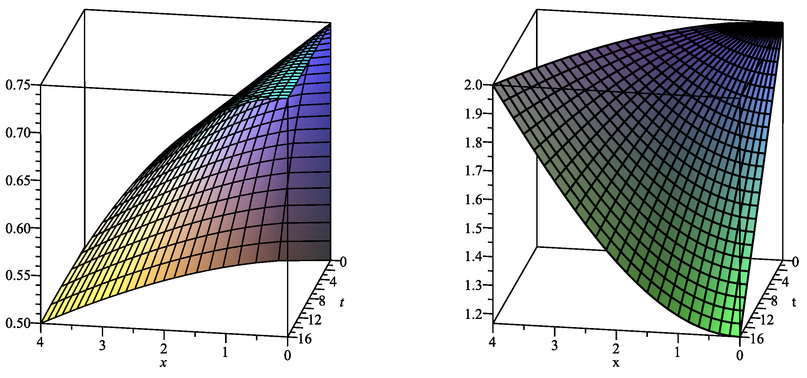
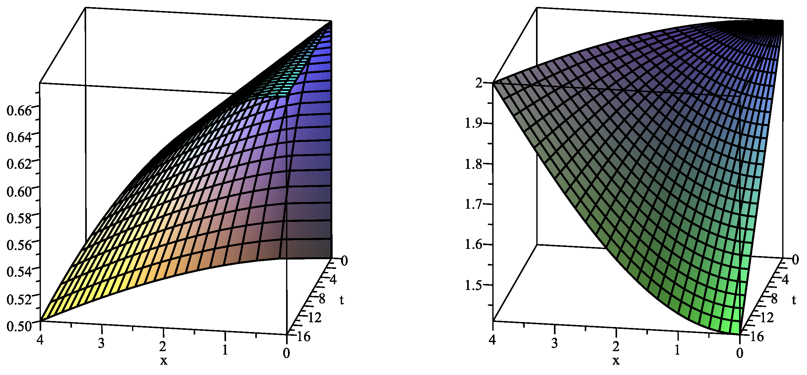
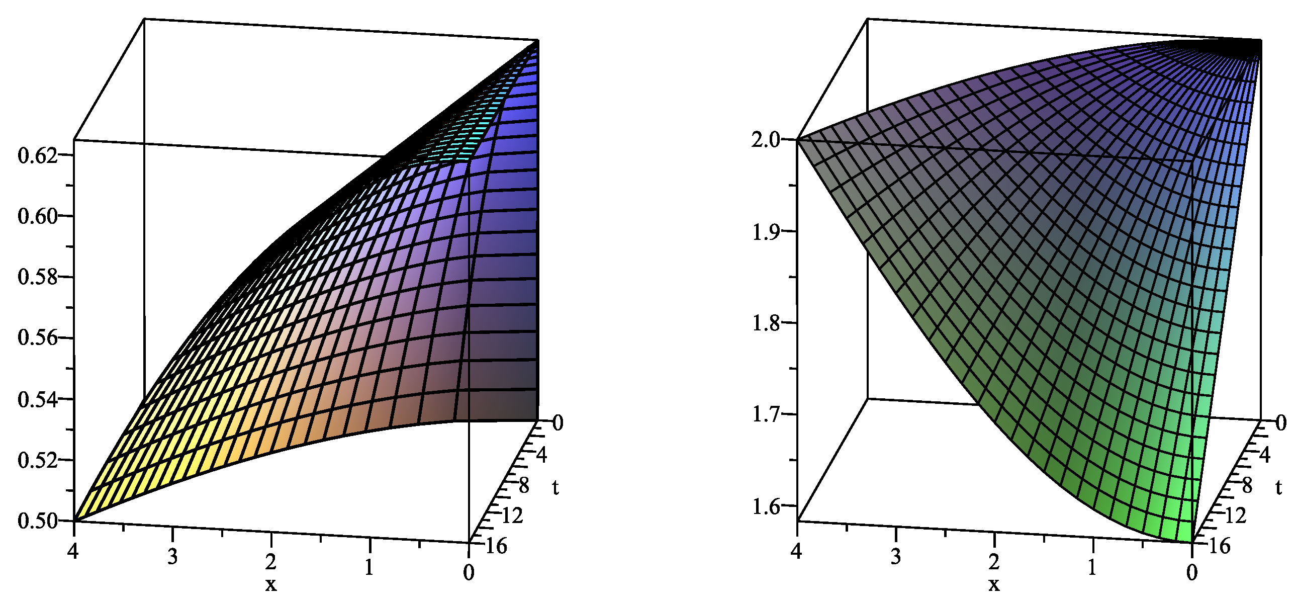
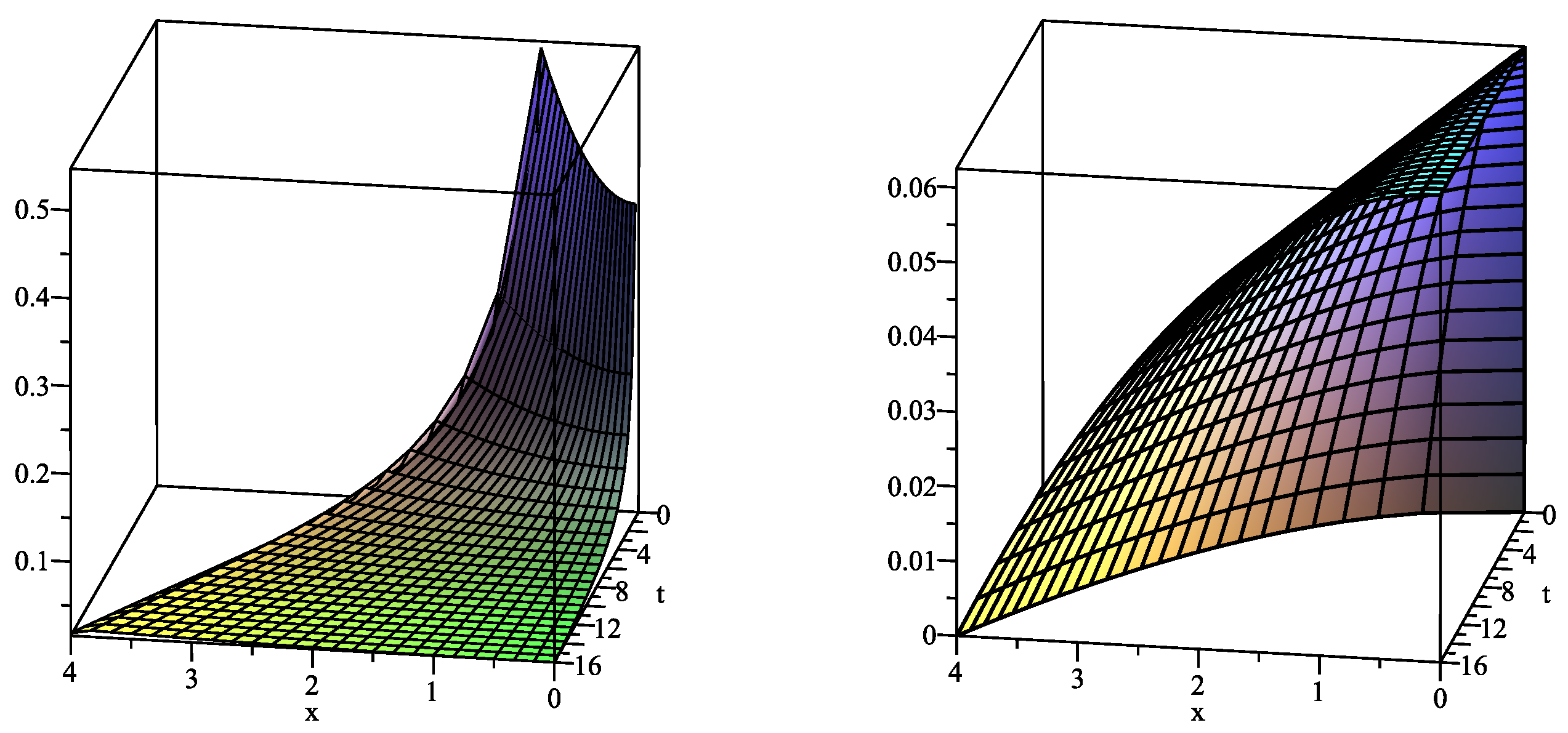
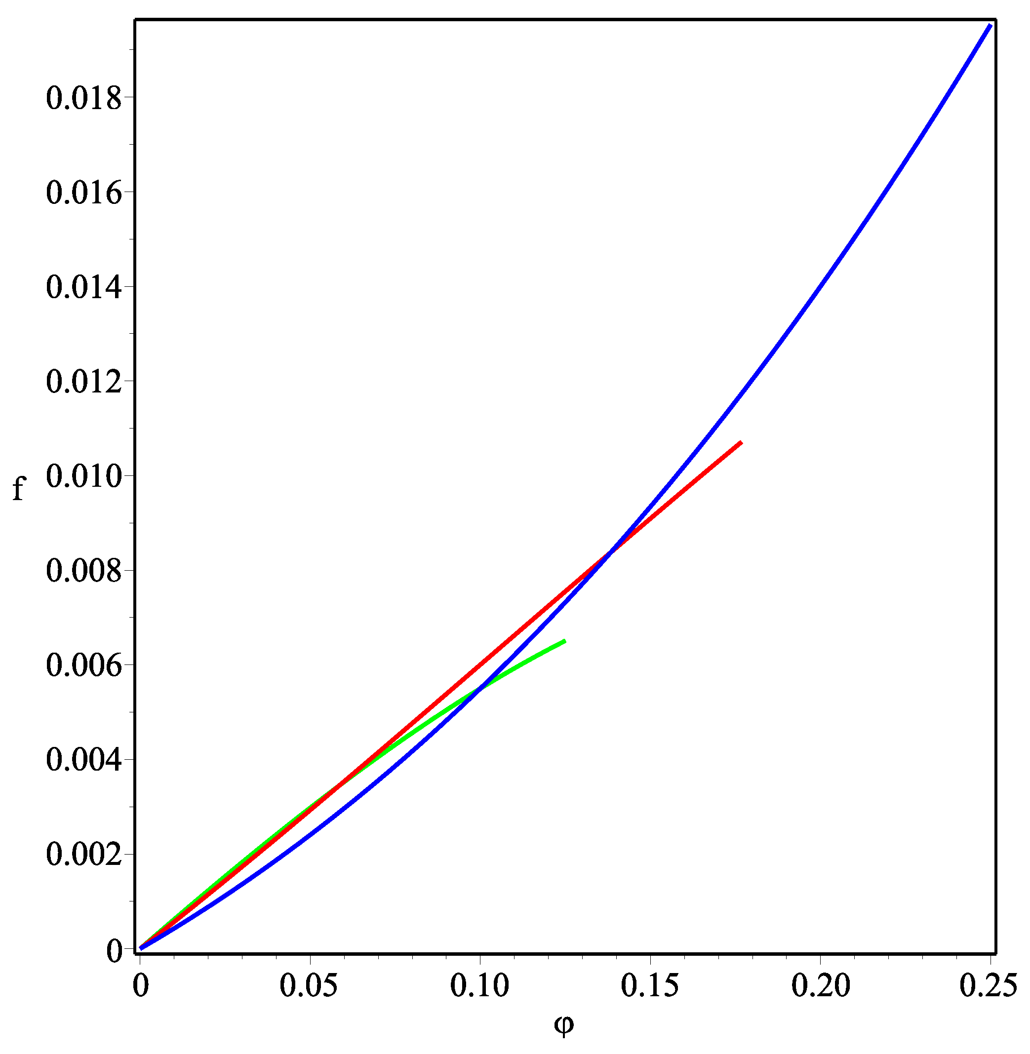
4. Boundary Value Problems for a One-Dimensional Tumour Growth Model with Negligible Cell Viscosity

In this section we apply the results of Lie symmetry classification derived in Section 2 for exact solving of a real world model proposed in [16] (see p. 570).

Consider the pressure difference with $r=1$ [16] (see p. 569 therein)

$$\mathsf{\Sigma }\left(\alpha \right)=k_0\frac{\alpha -{\alpha }_{*}}{{(1-\alpha )}^q}$$

assuming $\alpha >{\alpha }_{*}$. Setting

$$k\left(\alpha \right)=k_0{\alpha }^{1-m}{(1-\alpha )}^2\frac{d\left(\alpha \mathsf{\Sigma }\right)}{d\alpha }$$

the equation (see (23) in [16]) for the tumour cell concentration, $\alpha (t,x)$, takes the form

$${\alpha }_t={\left({\alpha }^m{\alpha }_x\right)}_x+S(\alpha ,c).$$

(40)

In order to simplify the boundary conditions we set

$$U=\alpha -{\alpha }_{*},V=c_{\infty }-c$$

(41)

(wherein c corresponds to the level of nutrient in [16], but might instead correspond to that of a chemotherapeutic drug) and arrive at the BVP

$$\begin{array}{c}{U}_t={\left({(U+{\alpha }_{*})}^m{U}_x\right)}_x+S(U+{\alpha }_{*},c_{\infty }-V),\hfill \\ 0=V_{xx}+Q(U+{\alpha }_{*},c_{\infty }-V),\hfill \\ x=0:U_x=V_x=0,\hfill \\ x=R\left(t\right):U=V=0,\hfill \\ x=R\left(t\right):\dot{R}=-{\alpha }_{*}^{m-1}{U}_x,\hfill \end{array}$$

(42)

where the concentrations $U(t,x)$ and $V(t,x)$ and the moving boundary location $R\left(t\right)$ are unknown functions, while the functions S and Q are given smooth functions, and m, ${\alpha }_{*}$ and $c_{\infty }$ are nonnegative parameters.

One may note that the governing equations of this BVP with $S=f\left(U\right)V^{-\beta }$ and $Q=g\left(U\right)V^{-\beta +1}$ are a particular case of case 2 in Table 1, so that they admit the Lie symmetry operator

$$X=2\beta t{\partial }_t+\beta x{\partial }_x+2V{\partial }_V.$$

(43)

It turns out that the following statement can be easily proved, using the definition of invariance for BVPs with moving boundaries [32].

Theorem 3.

The nonlinear BVP (42) with $S=f\left(U\right)V^{-\beta }$ and $Q=g\left(U\right)V^{-\beta +1}$ is invariant with respect to the two-dimensional MAI generated by the Lie symmetry operators (43) and ${\partial }_t$.

Clearly the time translation operator ${\partial }_t$ cannot help to find any realistic solutions of BVP (42), while the Lie symmetry (43) guarantees a reduction of the problem, which leads to some interesting results. In fact, the operator generates the ansatz

$$\begin{array}{c}U=\phi \left(\omega \right),\omega =\frac{x}{\sqrt{t}},\hfill \\ V=t^{\frac{1}{\beta }}\psi \left(\omega \right),\hfill \end{array}$$

(44)

which immediately specifies the function $R\left(t\right)={\omega }_0\sqrt{t}$ with the constant ${\omega }_0>0$ to be found. The reduced ODE problem is

$$\begin{array}{c}{(\phi +{\alpha }_{*})}^m{\phi }^{″}+m{(\phi +{\alpha }_{*})}^{m-1}{\left({\phi }^{\prime }\right)}^2+\frac{\omega }{2}{\phi }^{\prime }+f\left(\phi \right){\psi }^{-\beta }=0,\hfill \\ {\psi }^{″}+g\left(\phi \right){\psi }^{-\beta +1}=0,\hfill \\ \omega =0:{\phi }^{\prime }={\psi }^{\prime }=0,\hfill \\ \omega ={\omega }_0:\phi =\psi =0,{\phi }^{\prime }=-\frac{{\alpha }_{*}^{1-m}{\omega }_0}{2}.\hfill \end{array}$$

(45)

The nonlinear BVP (45) is still a complicated problem and we were unable to solve it analytically in general. Let us consider a special case, namely (45) with $\beta =1:$

$$\begin{array}{c}{(\phi +{\alpha }_{*})}^m{\phi }^{″}+m{(\phi +{\alpha }_{*})}^{m-1}{\left({\phi }^{\prime }\right)}^2+\frac{\omega }{2}{\phi }^{\prime }+f\left(\phi \right){\psi }^{-1}=0,\hfill \\ {\psi }^{″}+g\left(\phi \right)=0,\hfill \\ \omega =0:{\phi }^{\prime }={\psi }^{\prime }=0,\hfill \\ \omega ={\omega }_0:\phi =\psi =0,{\phi }^{\prime }=\frac{{\alpha }_{*}^{1-m}{\omega }_0}{2}.\hfill \end{array}$$

(46)

In this case the exact solution can be found for arbitrary m in the form

$$\begin{array}{c}\phi =\frac{{\alpha }_{*}^{1-m}}{4}\left({\omega }_0^2-{\omega }^2\right),\omega <{\omega }_0,\hfill \\ \psi =\frac{{\alpha }_{*}^{1-m}{q}_0}{48}\left({\omega }_0^2-{\omega }^2\right)\left(5{\omega }_0^2-{\omega }^2\right),\omega <{\omega }_0\hfill \end{array}$$

(47)

provided the functions $f\left(\phi \right)$ and $g\left(\phi \right)$ have the form

$$\begin{array}{c}g=q_0\phi ,q_0>0,\hfill \\ f=\frac{q_0{\alpha }_{*}^{m-1}}{3}\phi \left(\phi +{\alpha }_{*}^{1-m}{\omega }_0^2\right)\hfill \\ \times \left((m+\frac{1}{2}){\alpha }_{*}^{1-m}{(\phi +{\alpha }_{*})}^m-\frac{m{\alpha }_{*}^{2-m}}{4}\left({\alpha }_{*}^{-m}{\omega }_0^2+4\right){(\phi +{\alpha }_{*})}^{m-1}-\phi +\frac{{\alpha }_{*}^{1-m}}{4}{\omega }_0^2\right).\hfill \end{array}$$

(48)

Remark 3.

A similar result can be obtained for arbitrary diffusivity in the governing equation (40), i.e., the drag coefficient $k\left(\alpha \right)$, however, the structure of the function $f\left(\phi \right)$ will essentially depend on the diffusivity.

Now we present the final formulae for the original concentrations of tumour cells $\alpha (t,x)$ and nutrient (or drug) $c(t,x)$ using Formulae (41), ansatz (44) and solution (47):

$$\begin{array}{c}\alpha (t,x)={\alpha }_{*}+\frac{{\alpha }_{*}^{1-m}}{4}\left({\omega }_0^2-\frac{x^2}{t}\right),x<{\omega }_0\sqrt{t},\hfill \\ c(t,x)=c_{\infty }-\frac{{\alpha }_{*}^{1-m}{q}_0}{48}t\left({\omega }_0^2-\frac{x^2}{t}\right)\left(5{\omega }_0^2-\frac{x^2}{t}\right),x<{\omega }_0\sqrt{t},\hfill \\ R\left(t\right)={\omega }_0\sqrt{t}.\hfill \end{array}$$

(49)

Formulae (47) give the exact solution of the nonlinear BVP with a moving boundary for the governing equations

$$\begin{array}{c}{\alpha }_t={\left({\alpha }^m{\alpha }_x\right)}_x+\frac{f(\alpha -{\alpha }_{*})}{c-c_{\infty }},\hfill \\ 0=c_{xx}-q_0(\alpha -{\alpha }_{*}),\hfill \end{array}$$

(50)

and the boundary conditions

$$\begin{array}{c}x=0:{\alpha }_x=c_x=0,\hfill \\ x=R\left(t\right):\alpha ={\alpha }_{*},c=c_{\infty },\hfill \\ x=R\left(t\right):\dot{R}=-\frac{{\alpha }_x}{{\alpha }_{*}^{1-m}},\hfill \end{array}$$

(51)

where the function f is defined by (48), in particular one obtains the cubic polynomial for $m=0$:

$$f=\frac{q_0}{3{\alpha }_{*}}(\alpha -{\alpha }_{*})(\alpha -{\alpha }_1)({\alpha }_2-\alpha ),{\alpha }_1={\alpha }_{*}(1-{\omega }_0^2),{\alpha }_2={\alpha }_{*}\frac{6+{\omega }_0^2}{4},$$

(52)

hence

$$S(\alpha ,c)=\frac{q_0}{3{\alpha }_{*}}\frac{(\alpha -{\alpha }_{*})(\alpha -{\alpha }_1)({\alpha }_2-\alpha )}{c_{\infty }-c}.$$

(53)

This solution for some specified parameters is presented in Figure 1, Figure 2 and Figure 3. We note that the positive parameter ${\alpha }_{*}<1$ can be interpreted as a natural concentration of tumour cells, while $c_{\infty }$ is the concentration of nutrient (drug) in the medium surrounding the tumour. The positive parameter ${\omega }_0$ may be found from additional biologically motivated conditions. Notably the exact solution (49) can be easily generalised to one with two arbitrary parameters by the time translation $t\to t+t_0$.

It should be noted that the functions $f\left(\phi \right)$ and $g\left(\phi \right)$ in the cases $m=0$ (constant diffusion) and $m=1$ (as in the porous medium equation) are positive for the solution (47), meaning that the corresponding functions $S(\alpha ,c)$ and $Q(\alpha ,c)$ (see p. 570 in [16]) are positive (see an example in Figure 4). The cases $m\ne 0,1$ lead to a much more complicated structure for $f\left(\phi \right)$ and need to be examined separately for correctly-specified values of m. For example, the functions $S(\alpha ,c)$ and $Q(\alpha ,c)$ are positive on the solution for $m=1/2$ in the case of the parameters ${\alpha }_{*}=1/2$ and ${\omega }_0=1$ used in Figure 2.

We now turn to regimes in which the results may be susceptible to biological application, largely returning to the notation of [16]. The effective diffusivity of the cells is given by

$$D\left(\alpha \right)=\frac{\alpha }{k\left(\alpha \right)}{(1-\alpha )}^2\frac{d}{d\alpha }\left(\alpha \mathsf{\Sigma }\right).$$

(54)

The fact that cell-cell repulsion can be expected to increase at high densities implies that

$$\frac{d^2}{d{\alpha }^2}\left(\alpha \mathsf{\Sigma }\right)>0,$$

(55)

but this increasing contribution to (54) may be offset by the ${(1-\alpha )}^2$ prefactor (which itself will be less significant because $k\left(1\right)=0$ typically holds) that in part reflects the overall mass balance

$$\alpha v_c+(1-\alpha )v_w=0$$

(56)

between cell and water velocities, $v_c$ and $v_w$, respectively (so when $1-\alpha$ is small so typically is the cell velocity). The upshot is nevertheless that cases with $m\ge 0$ are those of most relevance, with increasing m corresponding to stronger cell-cell repulsion at high densities.

$S(\alpha ,c)$ will be positive when c represents a nutrient, with S an increasing function of c in both cases (corresponding to $\beta >0$ in the above). In this case, S will be an increasing function of $\alpha$ for sufficiently small $\alpha -{\alpha }_{*}$ (and linear in $\alpha$) and $S=0$ at $\alpha ={\alpha }_{*}$. One may note that the curves in Figure 5 satisfy these properties. In fact, all the curves represent increasing functions, the green and red curves in Figure 5 behave as linear functions, while the blue curve is linear for sufficiently small $\phi =\alpha -{\alpha }_{*}$ (the curves are built on the interval $[0,{\phi }_{max}]$ with ${\phi }_{max}$ prescribed by the first formula in (47)). Moreover, $f\left(\phi \right)=0$ for $\phi =0$ (see (48)). Notably, S may decrease again for larger $\alpha$, reflecting the limited supply of water to make new cells. The function S defined by (53) possesses such property provided $\alpha >{\alpha }_{max}\in ({\alpha }_{*},{\alpha }_2)$ , where ${\alpha }_{max}$ is a local maximum of f from (52) and can be easily calculated.

In the drug case, S would typically be taken positive for small c and negative for large c (with S a decreasing function of c)—this behaviour cannot be captured by the above nonlinearities, so in interpretation of the results, c should be regarded as everywhere sufficiently large that S is negative, again with $\beta >0$. Various dependencies on $\alpha$ can then be identified, and even $S=0$ at $\alpha =0$ need not hold (though additional constraints need to be imposed if $\alpha$ reaches zero).

Q should be positive in both interpretations (absorption, rather than generation, though the generation of toxic materials in the drug case could allow $Q<0$ to be contemplated) and an increasing function of c and $\alpha$. According to Theorem 3 $Q=g\left(U\right)V^{-\beta +1}$ (with U and V given in (41)), therefore one needs $\beta >1$ and an increasing function g in order to satisfy the above requirement.

$Q>0$ implies by the maximum principle that c will be an increasing function of x, having a minimum at $x=0$. Such behaviour of c is pictured in Figure 1, Figure 2 and Figure 3 for different values of m. The qualitative form of $\alpha$ will depend on the initial data and the form of S; in the case $S>0$, the nutrient supply is highest at the edge of the tumour, but $\alpha$ is held at ${\alpha }_{*}$ there by the stress balance (more water is taken up to prevent $\alpha$ exceeding ${\alpha }_{*}$ due to cell division), so, perhaps counterintuitively, it is quite possible for $\alpha$ to be maximal at $x=0$ if S remains sufficiently large, despite the decrease in c. However, such behaviour is more natural for $S<0$ (the drug case) since the cell-kill rate can be expected to be highest at the edge of the tumour.

5. Higher-Dimensional Tumour Growth Model without Cell Viscosity

In Section 4, we examined the one-dimensional model (42) describing the tumour growth. Here we generalise the model to higher dimensions under the assumption that tumour cells create a radially symmetrical shape (a circular cylinder for $n=1$ and a sphere for $n=2$). In this case, the nonlinear BVP (42) takes the following form:

$$\begin{array}{c}{U}_t=\frac{1}{r^n}{\left(r^n{(U+{\alpha }_{*})}^m{U}_r\right)}_r+S(U+{\alpha }_{*},c_{\infty }-V),\hfill \\ 0=\frac{1}{r^n}{\left(r^n{V}_r\right)}_r+Q(U+{\alpha }_{*},c_{\infty }-V),\hfill \\ r=0:U_r=V_r=0,\hfill \\ r=R\left(t\right):U=V=0,\hfill \\ r=R\left(t\right):\dot{R}=-{\alpha }_{*}^{m-1}{U}_r,\hfill \end{array}$$

(57)

where $n=1,2$ and the same notations are used as in Section 4, however, the space variable x is replaced by the variable $r=\sqrt{x_1^2+\cdots +x_n^2+x_{n+1}^2}$.

One may check that the governing equations of this BVP with $S=f\left(U\right)V^{-\beta }$ and $Q=g\left(U\right)V^{-\beta +1}$ are invariant w.r.t. the Lie symmetry operator

$$X=2\beta t{\partial }_t+\beta r{\partial }_r+2V{\partial }_V,$$

(58)

which has the same structure as (43).

Theorem 4.

The nonlinear BVP (57) with $S=f\left(U\right)V^{-\beta }$ and $Q=g\left(U\right)V^{-\beta +1}$ is invariant with respect to the two-dimensional MAI generated by the Lie symmetry operators (58) and ${\partial }_t$.

Thus, the Lie symmetry (58) generates the ansatz

$$\begin{array}{c}U=\phi \left(\omega \right),\omega =\frac{r}{\sqrt{t}},\hfill \\ V=t^{\frac{1}{\beta }}\psi \left(\omega \right),\hfill \end{array}$$

(59)

which immediately specifies the function $R\left(t\right)={\omega }_0\sqrt{t}$ and reduces the two-dimensional BVP (57) (with $S=f\left(U\right)V^{-\beta }$ and $Q=g\left(U\right)V^{-\beta +1}$) to the one-dimensional problem

$$\begin{array}{c}{(\phi +{\alpha }_{*})}^m{\phi }^{\prime \prime }+m{(\phi +{\alpha }_{*})}^{m-1}{\left({\phi }^{\prime }\right)}^2+\frac{n}{\omega }{(\phi +{\alpha }_{*})}^m{\phi }^{\prime }+\frac{\omega }{2}{\phi }^{\prime }+f\left(\phi \right){\psi }^{-\beta }=0,\hfill \\ {\psi }^{″}+\frac{n}{\omega }{\psi }^{\prime }+g\left(\phi \right){\psi }^{-\beta +1}=0,\hfill \\ \omega =0:{\phi }^{\prime }={\psi }^{\prime }=0,\hfill \\ \omega ={\omega }_0:\phi =\psi =0,{\phi }^{\prime }=-\frac{{\alpha }_{*}^{1-m}{\omega }_0}{2}.\hfill \end{array}$$

(60)

The nonlinear problem (60) is still not integrable for arbitrary given coefficients, however, one with $\beta =-1$ is again a solvable case. Direct calculations show that Formulae (47) and (48) can be generalised in this case as follows

$$\begin{array}{c}\phi =\frac{{\alpha }_{*}^{1-m}}{4}\left({\omega }_0^2-{\omega }^2\right),\omega <{\omega }_0,\hfill \\ \psi =\frac{{\alpha }_{*}^{1-m}{q}_0}{16(n+3)}\left({\omega }_0^2-{\omega }^2\right)\left(\frac{n+5}{n+1}{\omega }_0^2-{\omega }^2\right),\omega <{\omega }_0\hfill \end{array}$$

(61)

and

$$\begin{array}{c}g=q_0\phi ,q_0>0,\hfill \\ f=\frac{q_0{\alpha }_{*}^{m-1}}{n+3}\phi \left(\phi +\frac{{\alpha }_{*}^{1-m}{\omega }_0^2}{n+1}\right)\hfill \\ \times \left((m+\frac{n+1}{2}){\alpha }_{*}^{1-m}{(\phi +{\alpha }_{*})}^m-\frac{m{\alpha }_{*}^{2-m}}{4}\left({\alpha }_{*}^{-m}{\omega }_0^2+4\right){(\phi +{\alpha }_{*})}^{m-1}-\phi +\frac{{\alpha }_{*}^{1-m}}{4}{\omega }_0^2\right).\hfill \end{array}$$

(62)

In order to obtain the final formulae for the original concentrations of tumour cells $\alpha (t,x)$ and nutrient (drug) $c(t,x)$, we use Formulae (41), ansatz (59) and solution (61). The formulae obtained coincide with those presented in (49) for $\alpha (t,x)$ and $R\left(t\right)$ while for the nutrient (drug) concentration we have the solution

$$c(t,r)=c_{\infty }-\frac{{\alpha }_{*}^{1-m}{q}_0}{16(n+3)}t\left({\omega }_0^2-\frac{r^2}{t}\right)\left(\frac{n+5}{n+1}{\omega }_0^2-\frac{r^2}{t}\right),r<{\omega }_0\sqrt{t}.$$

(63)

The biomedical interpretation of the various regimes coincides with that in Section 4 and is omitted here.

6. Conclusions

The main part of this paper is devoted to the Lie symmetry classification of the class of parabolic-elliptic systems (3). First of all, the structure of form-preserving (admissible) transformations for the systems of the form (3) is established (see Theorem 1) in order to establish possible relations between systems that admit equivalent MAIs. Theorem 2 gives a complete list of inequivalent parabolic-elliptic systems consisting of 35 systems, which are invariant under nontrivial MAIs, i.e., under the three- and higher-dimensional Lie algebras. Moreover, we have established all possible subclasses of parabolic-elliptic systems (see Table 3 and Table 4) with nontrivial Lie symmetry, which are reducible to those listed in Table 1 and Table 2 by the relevant form-preserving transformations. Notably, our result is a new confirmation of importance of finding form-preserving transformations because they allow reducing essentially (in contrast to the group of equivalence transformations) the number of inequivalent systems. In fact, the traditional Lie–Ovsiannikov algorithm, which is based on the group of equivalence transformations, would lead to 57 parabolic-elliptic systems instead of 35 systems listed in Table 1 and Table 2 because 22 systems from Table 3 and Table 4 should be added.

From the applicability point of view, the most interesting parabolic-elliptic systems occur in Table 1 because the systems from Table 2 are semi-coupled. It is worth noting that MAIs for the systems arising in all the cases of Table 1 excepting 7 and 14 are some analogs of those for single RD equations. In fact, fixing the diffusion coefficient in the first equation of the corresponding system one may easily identify its generic analog in Table 4 [24] (see cases 3–5 and 7 therein). For example, MAIs of the systems from cases 8 and 9 contain the well-known algebra $sl(2,\mathbb{R})$ as a subalgebra (see the second, third and fourth operators in the last column). The same subalgebra occurs for the diffusion equation with the same diffusivity (see case 3 in Table 4 [24]). By the way, Ovsiannikov was the first to identify this special case for nonlinear diffusion equations [17]. Of course, the systems in Table 1 have more general structures (many of them contain arbitrary functions as coefficients) in contrast to their analogs listed in Table 4 [24]. However, it happens on a regular basis if one considers systems instead of single equations (see, e.g., case 10 in Table 1 [13] involving the same diffusivity).

Cases 7 and 14 in Table 1 have no analogs among single RD equations. Moreover, the relevant MAIs generate infinite-dimensional Lie algebras because they contain the operators $X^{\infty }$ involving an arbitrary smooth function $\phi \left(t\right)$ (see the last column of Table 1). Interestingly, both MAIs from Cases 7 and 14 again contain the well-known algebra $sl(2,\mathbb{R})$ as a subalgebra. In fact, if one sets $\phi \left(t\right)=t$ and $\phi \left(t\right)=t^2$ then the operators ${\partial }_t$, $X^{\infty }$ with $\phi \left(t\right)=t$ and $X^{\infty }$ with $\phi \left(t\right)=t^2$ produce nothing else but $sl(2,\mathbb{R})$ with new representations (it is a simple task to check the commutator relations), which do not happen in the case of single RD equations.

In order to demonstrate applicability of our pure theoretical result, we apply the Lie symmetry corresponding to one-parameter group of scale transformation for solving a (1+1)-dimensional BVP with a free boundary modeling tumour growth [16]. We reduce the given nonlinear BVP to that governed by ODEs. As a result, its exact solution was constructed under additional restrictions on the coefficients arising in the governing equations. Moreover, possible biological interpretations of the solution are discussed. In particular, it was shown that the results obtained allow plausible interpretation in the case when the model describes growth of tumour cells consuming a nutrient. Finally, the results for the above (1+1)-dimensional BVP were generalised on multi-dimensional case under the assumption that tumour cells create a radially symmetrical shape. In a forthcoming paper, we will generalise these results using the definition of conditional invariance for BVPs introduced in [33].

References

1. Ames, W.F. Nonlinear Partial Differential Equations in Engineering; Academic: New York, NY, USA, 1972; ISBN 9780080955247. [Google Scholar]
2. Murray, J.D. Mathematical Biology; Springer: Berlin, Germany, 1989. [Google Scholar]
3. Murray, J.D. Mathematical Biology, II: Spatial Models and Biomedical Applications; Springer: Berlin, Germany, 2003. [Google Scholar]
4. Okubo, A.; Levin, S.A. Diffusion and Ecological Problems. Modern Perspectives, 2nd ed.; Springer: Berlin, Germany, 2001. [Google Scholar]
5. Lotka, A.J. Undamped oscillations derived from the law of mass action. J. Am. Chem. Soc. 1920, 42, 1595–1599. [Google Scholar] [CrossRef]
6. Volterra, V. Variazionie fluttuazioni del numero d’individui in specie animali conviventi. Mem. Acad. Lincei 1926, 2, 31–113. (In Italian) [Google Scholar]
7. Turing, A.M. The chemical basis of morphogenesis. Philos. Trans. R. Soc. B 1952, 237, 37–72. [Google Scholar] [CrossRef]
8. Zulehner, W.; Ames, W.F. Group analysis of a semilinear vector diffusion equation. Nonlinear Anal. 1983, 7, 945–969. [Google Scholar] [CrossRef]
9. Cherniha, R.; King, J.R. Lie symmetries of nonlinear multidimensional reaction-diffusion systems: I. J. Phys. A Math. Gen. 2000, 33, 267–282. [Google Scholar] [CrossRef]
10. Cherniha, R.; King, J.R. Addendum: Lie symmetries of nonlinear multidimensional reaction-dfiffusion systems: I. J. Phys. A Math. Gen. 2000, 33, 7839–7841. [Google Scholar] [CrossRef]
11. Cherniha, R.; King, J.R. Lie symmetries of nonlinear multidimensional reaction-diffusion systems: II. J. Phys. A Math. Gen. 2003, 36, 405–425. [Google Scholar] [CrossRef]
12. Knyazeva, I.V.; Popov, M.D. A system of two diffusion equations. In CRC Handbook of Lie Group Analysis of Differential Equations; CRC Press: Boca Raton, FL, USA, 1994; Volume 1, pp. 171–176. [Google Scholar]
13. Cherniha, R.; King, J.R. Non-linear reaction-diffusion systems with variable diffusivities: Lie symmetries, ansatze and exact solutions. J. Math. Anal. Appl. 2005, 308, 11–35. [Google Scholar] [CrossRef]
14. Cherniha, R.; King, J.R. Lie symmetries and conservation laws of non-linear multidimensional reaction–diffusion systems with variable diffusivities. IMA J. Appl. Math. 2006, 71, 391–408. [Google Scholar] [CrossRef]
15. Torrisi, M.; Tracina, R. An application of equivalence transformations to reaction diffusion equations. Symmetry 2015, 7, 1929–1944. [Google Scholar] [CrossRef]
16. Byrne, H.; King, J.R.; McElwain, D.L.S.; Preziosi, L. A two-phase model of solid tumour growth. Appl. Math. Lett. 2003, 16, 567–573. [Google Scholar] [CrossRef]
17. Ovsiannikov, L.V. Group relations of the equation of non-linear heat conductivity. Dokl. Akad. Nauk SSSR 1959, 125, 492–495. (In Russian) [Google Scholar]
18. Kingston, J.G. On point transformations of evolution equations. J. Phys. A Math. Gen. 1991, 24, L769–L774. [Google Scholar] [CrossRef]
19. Kingston, J.G.; Sophocleous, C. On form-preserving point transformations of partial differential equations. J. Phys. A Math. Gen. 1998, 31, 1597–1619. [Google Scholar] [CrossRef]
20. Niederer, U. Schrödinger invariant generalised heat equation. Helv. Phys. Acta 1978, 51, 220–239. [Google Scholar]
21. Gazeau, J.P.; Winternitz, P. Symmetries of variable coefficient Korteweg-de Vries equations. J. Math. Phys. 1992, 33, 4087–4102. [Google Scholar] [CrossRef]
22. Ames, W.F.; Anderson, R.L.; Dorodnitsyn, V.A.; Ferapontov, E.V.; Gazizov, R.K.; Ibragimov, N.H.; Svirshchevskiy, S.R. CRC Handbook of Lie Group Analysis of Differential Equations, vol. 1. Symmetries, Exact Solutions And Conservation Laws; CRC Press: Boca Raton, FL, USA, 1994; pp. 133–136. [Google Scholar]
23. Cherniha, R.; Serov, M. Symmetries, ansätze and exact solutions of nonlinear second-order evolution equations with convection term. Eur. J. Appl. Math. 1998, 9, 527–542. [Google Scholar] [CrossRef]
24. Cherniha, R.; Serov, M.; Rassokha, I. Lie symmetries and form-preserving transformations of reaction-diffusion-convection equations. J. Math. Anal. Appl. 2008, 342, 1363–1379. [Google Scholar] [CrossRef]
25. Cherniha, R.; Serov, M.; Pliukhin, O. Nonlinear Reaction-Diffusion-Convection Equations: Lie and Conditional Symmetry, Exact Solutions and Their Applications; CRC Press Taylor and Francis Group: Boka Raton, FL, USA, 2018; ISBN 9781498776172. [Google Scholar]
26. Cherniha, R.; Davydovych, V. Reaction-diffusion systems with constant diffusivities: Conditional symmetries and form-preserving transformations. In Algebra, Geometry and Mathematical Physics; Springer: Berlin/Heidelberg, Germany, 2014; Volume 85, pp. 533–553. [Google Scholar]
27. Arrigo, D.J. Symmetry Analysis of Differential Equations: An Introduction; John Wiley and Sons: Hoboken, NJ, USA, 2015; ISBN 9781118721445. [Google Scholar]
28. Bluman, G.W.; Anco, S.C. Symmetry and Integration Methods for Differential Equations; Springer: New York, NY, USA, 2002; ISBN 9780387216492. [Google Scholar]
29. Bluman, G.W.; Kumei, S. Symmetries and Differential Equations; Springer: Berlin, Germany, 1989. [Google Scholar]
30. Fushchych, W.I.; Shtelen, W.M.; Serov, M.I. Symmetry Analysis and Exact Solutions of Equations of Nonlinear Mathematical Physics; Kluwer: Dordrecht, The Netherlands, 1993. [Google Scholar]
31. Olver, P.J. Applications of Lie Groups to Differential Equations; Springer: Berlin, Germany, 1986; ISBN 978-1-4684-0274-2. [Google Scholar]
32. Cherniha, R.; Kovalenko, S. Lie symmetries and reductions of multi-dimensional boundary value problems of the Stefan type. J. Phys. A Math. Theor. 2011, 44, 485202. [Google Scholar] [CrossRef]
33. Cherniha, R.; King, J.R. Lie and Conditional Symmetries of a Class of Nonlinear (1 + 2)—Dimensional Boundary Value Problems. Symmetry 2015, 7, 1410–1435. [Google Scholar] [CrossRef]
Figure 1. Surfaces representing the concentrations α (left) and c (right) of the form (49) for the parameter values m = 1 , α * = 0.5 , c = 2 , ω 0 = 1 , q 0 = 0.5 .
Symmetry 10 00171 g001
Figure 2. Surfaces representing the concentrations α (left) and c (right) of the form (49) for the parameter value m = 0.5 (other parameters as in Figure 1).
Symmetry 10 00171 g002
Figure 3. Surfaces representing the concentrations α (left) and c (right) of the form (49) for the parameter value m = 0 (other parameters as in Figure 1).
Symmetry 10 00171 g003
Figure 4. Surfaces representing the function S ( α ( t , x ) , c ( t , x ) ) (left) and Q ( α ( t , x ) , c ( t , x ) ) (right) on the known concentrations given by (49) (other parameters as in Figure 3).
Symmetry 10 00171 g004
Figure 5. Curves representing the functions f ( φ ) (48) for parameters m = 0 (green), m = 0.5 (red) and m = 1 (blue). The other parameters are as in Figure 1.
Symmetry 10 00171 g005