Picture Hesitant Fuzzy Set and Its Application to Multiple Criteria Decision-Making

Abstract

To address the complex multiple criteria decision-making (MCDM) problems in practice, this article proposes the picture hesitant fuzzy set (PHFS) theory based on the picture fuzzy set and the hesitant fuzzy set. First, the concept of PHFS is put forward, and its operations are presented, simultaneously. Second, the generalized picture hesitant fuzzy weighted aggregation operators are developed, and some theorems and reduced operators of them are discussed. Third, the generalized picture hesitant fuzzy prioritized weighted aggregation operators are put forward to solve the MCDM problems that the related criteria are at different priorities. Fourth, two novel MCDM methods combined with the proposed operators are constructed to determine the best alternative in real life. Finally, two numerical examples and an application of web service selection are investigated to illustrate the effectiveness of the proposed methods. The sensitivity analysis shows that the different values of the parameter $\lambda$ affect the ranking of alternatives, and the proposed operators are compared with several existing MCDM methods to illustrate their advantages.

1. Introduction

Multiple criteria decision-making (MCDM) problems occur in numerous practical fields [1,2,3]. For a specific purpose, several possible plans may be presented as the alternatives; then, decision makers assess the alternatives concerning the related criteria to determine the best one. Traditionally, crisp numbers are utilized to express the evaluation information. However, in real life, the data are inevitably incomplete and complex, and decision makers may be uncertain when evaluating the alternatives. To deal with the fuzziness of evaluation information, the fuzzy set (FS) [4] was proposed to improve the information form. During the past decades, many scholars devoted themselves to the study of the fuzzy MCDM problems [1]. Furthermore, in recent years, along with the complexity of the MCDM problems, how to improve the FS theory to deal with different specific situations has been a hot topic.

Although FS is a valid form to express the uncertain evaluation information, it cannot solve several complex situations in real life. For more effective expression of the evaluation information, many generalized forms of FS were proposed [5,6,7,8,9,10]. The purpose of this paper is to propose a new information form; the picture hesitant fuzzy set (PHFS) theory is put forward combined with the concepts of picture fuzzy set (PFS) [7] and hesitant fuzzy set (HFS) [8]. As a generalized form of FS, intuitionistic fuzzy set (IFS) [5], PFS, and HFS, PHFS can express the uncertainty and complexity of human opinions in practice; furthermore, the positive, neutral, negative, and refusal membership degrees are represented by several possible values that are given by decision makers.

In practice, the uncertain and complex evaluation information will be inevitably given by decision makers. For example, ten business managers discuss an investment project; five suggest agreement, two present disagreement, and the other business managers choose to abstain. Obviously, FS can only indicate the membership degree of evaluation information; thus, the opinions of the 10 business managers cannot be represented by FS. For overcoming the limitation of FS, Atanassov [5] put forward the non-membership function and developed the IFS. Then, the evaluation information in the aforementioned example can be expressed by IFS accurately. Later, the interval numbers were used to substitute the crisp numbers in IFS; then, the interval-valued intuitionistic fuzzy set (IVIFS) was developed [6]. To convey the indeterminate information of decision makers more effectively, Ye [9] and Liu and Yuan [11] extended the FS to triangular and trapezoidal intuitionistic fuzzy set, respectively. However, in some particular situations, it is not convincing to represent the evaluation information combined with IFS or IVIFS. For instance, there is a vote for a specific matter, the voting opinions of voters can be divided into four types, namely, vote for, abstain, vote against, and a refusal of the voting [12]. Therefore, Cuong [7,13] put forward the PFS, which is composed by the positive, neutral, negative, and refusal membership functions; thus, PFS can express the opinions of decision makers accurately in the example above. Subsequently, the correlation coefficient, distance measure, and cross-entropy measure of PFS were investigated in detail [14,15,16].

On the other hand, sometimes the accurate membership degree of evaluation information is difficult to be determined, which is also another shortcoming of FS. Therefore, the HFS was developed [17], in which the membership degrees are represented by several possible crisp numbers. Next, the interval numbers were introduced to extend the membership function of HFS and the interval-valued hesitant fuzzy set (IVHFS) theory was proposed [18]. According to the IFS and HFS, several potential membership and non-membership functions were expressed to put forward the dual hesitant fuzzy set (DHFS) [10]. Later, Farhadinia [19] constructed the dual interval-valued hesitant fuzzy set (DIVHFS) combined with DHFS. Nevertheless, HFS in the existing research cannot express all types of human opinions in the aforementioned example.

According to the evaluation information of the individual decision makers, the collective evaluation information of each alternative is obtained through the information fusion. Due to the important role of aggregation tools in MCDM problems, many scholars have investigated the aggregation operators of different fuzzy information. For example, Xu and Yager [20] developed the operations of intuitionistic fuzzy numbers (IFNs) and proposed the intuitionistic fuzzy geometric aggregation operators. Later, Xu [21] put forward the intuitionistic fuzzy weighted averaging aggregation operators to aggregate the IFNs. Next, several interval-valued intuitionistic fuzzy aggregation operators were constructed to deal with the MCDM [22,23,24]. With respect to the picture fuzzy (PF) evaluation information, Wei [25] defined the operations of picture fuzzy numbers (PFNs) according to the study of [21] and proposed the picture fuzzy weighted aggregation operators. In addition, several PF aggregation operators according to different operations were put forward [12,26]. Besides, a great time of hesitant fuzzy aggregation operators and their generalized forms were constructed [27], and several aggregation operators under dual hesitant fuzzy and dual interval-valued hesitant fuzzy environment were developed [28,29,30].

In some practical MCDM problems, the related criteria may be at different priority levels. For instance, a young couple wants to choose a toy for their child, the criteria of the toy they will consider are safety and price; obviously, the criteria safety has a higher priority than price. However, the aforementioned aggregation operators cannot fuse the aggregated arguments that are in different priority levels. In response to these situations, Yager [31] proposed the prioritized averaging (PA) operator. Inspired by Yager [31], Yu et al. [32,33] constructed the intuitionistic fuzzy prioritized fuzzy and interval-valued intuitionistic fuzzy prioritized fuzzy aggregation operators. Besides, the hesitant fuzzy prioritized aggregation operators were proposed to aggregate the evaluation information that is at different priorities [34]. Nevertheless, to our best knowledge, few researches have extended the PA operator to solve the MCDM problems under PF environment.

In summary, this paper defines the PHFS based on the PFS and HFS and develops the operations laws of picture hesitant fuzzy elements (PHFEs) according to the operations of IFNs [21]. Then, the generalized picture hesitant fuzzy aggregation operators and generalized picture hesitant fuzzy prioritized aggregation operators are put forward, and the properties and reduced operators of them are investigated. Furthermore, the proposed operators are utilized to solve diverse situations during MCDM processes under picture hesitant fuzzy (PHF) environment.

The rest of this paper is structured as follows. Definitions of the PFS, HFS, and PA operator are presented in Section 2. The concept of PHFS is defined, and the comparison method and operations of PHFEs are proposed in Section 3. Section 4 constructs the generalized picture hesitant fuzzy weighted averaging (GPHFWA), generalized picture hesitant fuzzy weighted geometric (GPHFWG), generalized picture hesitant fuzzy prioritized weighted averaging (GPHFPWA), and generalized picture hesitant fuzzy prioritized weighted geometric (GPHFPWG) operators. In Section 5, two MCDM methods are constructed according to the proposed operators. Section 6 applies the proposed methods into two numerical examples and an application of web service selection to show the effectiveness and advantages of the proposed methods. Finally, some conclusions are summarized in Section 7.

2. Preliminaries

To make this paper as self-contained as possible, we recall the definitions of the PFS, HFS, and PA operator, which will be utilized in the subsequent research.

2.1. PFS

Atanassov [5] applied the non-membership degree to extend FS; however, expressing the evaluation information depend on IFS is unreasonable in practice, at times. Therefore, Cuong [13] proposed the PFS theory based on FS and IFS, which can represent more information of decision makers, including yes, abstain, no, and refusal.

Definition 1.

Let$X$be a non-empty and finite set, a PFS$P$on$X$ is defined by

$$P=\left\{\langle x,{\mu }_P\left(x\right),{\eta }_P\left(x\right),v_P\left(x\right)\rangle |x\in X\right\},$$

(1)

where ${\mu }_P\left(x\right)$, ${\eta }_P\left(x\right)$, and $v_P\left(x\right)$ are the positive, neutral, and negative membership functions that are belonging to $\left[0,1\right]$, respectively, and they meet the condition of $0\le {\mu }_P\left(x\right)+{\eta }_P\left(x\right)+v_P\left(x\right)\le 1$. Furthermore, ${\pi }_P\left(x\right)=1-{\mu }_P\left(x\right)-{\eta }_P\left(x\right)-v_P\left(x\right)$ is the refusal membership function.

Definition 2.

A picture fuzzy number (PFN) is represented by$a=\left({\mu }_a,{\eta }_a,v_a\right)$, where${\mu }_a\in \left[0,1\right]$,${\eta }_a\in \left[0,1\right]$,$v_a\in \left[0,1\right]$, and${\mu }_a+{\eta }_a+v_a\le 1$[25].

Wei [25] proposed the operations of PFNs based on the operations of IFNs in [21].

Definition 3.

Let$a_1=\left({\mu }_1,{\eta }_1,v_1\right)$,$a_2=\left({\mu }_2,{\eta }_2,v_2\right)$, and$a=\left(\mu ,\eta ,v\right)$be three PFNs,$\lambda >0$, and$a^c$is the complementary set of$a$, then [25]

$$a^c=\left(v,\eta ,\mu \right);$$

(2)

$$a_1\oplus a_2=\left({\mu }_1+{\mu }_2-{\mu }_1{\mu }_2,{\eta }_1{\eta }_2,v_1{v}_2\right);$$

(3)

$$a_1\otimes a_2=\left({\mu }_1{\mu }_2,{\eta }_1+{\eta }_2-{\eta }_1{\eta }_2,v_1+v_2-v_1{v}_2\right);$$

(4)

$$\lambda a=\left(1-{\left(1-\mu \right)}^{\lambda },{\eta }^{\lambda },v^{\lambda }\right);$$

(5)

$$a^{\lambda }=\left({\mu }^{\lambda },1-{\left(1-\eta \right)}^{\lambda },1-{\left(1-v\right)}^{\lambda }\right).$$

(6)

2.2. HFS

Due to the complexity of the evaluated object in practice, decision makers may have difficulty determining an accurate value of the membership level. To deal with this situation, Torra [8] developed the HFS theory in which the membership degree is expressed by several possible values.

Definition 4.

Let$\wp \left(\left[0,1\right]\right)$be the set of all subsets of the unitary interval and$X$be a non- empty set. Let$h_A:X\to \wp \left(\left[0,1\right]\right)$, then an HFS$A$on$X$ is defined by

$$A=\left\{\langle x,h_A\left(x\right)\rangle |x\in X\right\}.$$

(7)

Definition 5.

A hesitant fuzzy element (HFE) is a non-empty and finite subset of$\left[0,1\right]$ [27].

Although a HFE can be given by any subset of $\left[0,1\right]$, in practice, HFS is commonly restricted to finite set in the MCDM problems [27]. Therefore, Bedregal at al. [35] proposed the typical hesitant fuzzy set (THFS), which is the finite and non-empty HFS. Later, Alcantud and Torra [36] defined the uniformly typical hesitant fuzzy set (UTHFS) that can simplify many theoretical and practical arguments, which is a generalized form of THFS. In this paper, the evaluation information of decision makers is expressed by UTHFS during the MCDM processes under hesitant fuzzy environment.

Definition 6.

Let$\mathrm{H}\subseteq \wp \left(\left[0,1\right]\right)$be the set of all finite and non-empty subsets of$\left[0,1\right]$, and let$X$be a non- empty set. Then, a THFS$A$on$X$is defined by Equation (7), where$h_A:X\to \mathrm{H}$. Each$h\in \mathrm{H}$ is called a typical hesitant fuzzy element (THFE) [35].

Definition 7.

Let$A$be a THFS on$X$, if there is$N$such that the cardinality of the THFS$l_A\left(x\right)\le N$for each$x\in X$. Then, the THFS$A$is an UTHFS. Each$h\in \mathrm{H}$ is called an uniformly typical hesitant fuzzy element (UTHFE) [36].

To aggregate the hesitant fuzzy evaluation information, Xia and Xu [27] investigated the operations of HFEs, which is also valid for fusing UTHFEs.

Definition 8.

Let$h$,$h_1$, and$h_2$be three UTHFEs,$\lambda >0$, then

$$h_1\oplus h_2={\displaystyle \underset{{\gamma }_1\in h_1,{\gamma }_2\in h_2}{\cup }\left\{{\gamma }_1+{\gamma }_2-{\gamma }_1{\gamma }_2\right\}};$$

(8)

$$h_1\otimes h_2={\displaystyle \underset{{\gamma }_1\in h_1,{\gamma }_2\in h_2}{\cup }\left\{{\gamma }_1{\gamma }_2\right\}};$$

(9)

$$\lambda h={\displaystyle \underset{\gamma \in h}{\cup }\left\{1-{\left(1-\gamma \right)}^{\lambda }\right\}};$$

(10)

$$h^{\lambda }={\displaystyle \underset{\gamma \in h}{\cup }\left\{{\gamma }^{\lambda }\right\}}.$$

(11)

2.3. The PA Operator

Aggregation operator plays a crucial role in the process of information fusion. Sometimes, the criteria have different priorities according to their important degree; thus, Yager [31] constructed the PA operator to address these situations.

Definition 9.

Let$C=\left\{C_1,C_2,\dots ,C_n\right\}$ be a set of criteria, which are divided into several priority levels, i.e., the priority of $C_p$is higher than$C_q$when$p<q$. The$C_j\left(x\right)\in \left[0,1\right]$is the evaluation value of the alternative$x$concerning the criteria$C_j$. Thus, the PA operator is expressed by

$$PA\left(C_1\left(x\right),C_2\left(x\right),\dots ,C_n\left(x\right)\right)={\displaystyle \sum _{j=1}^n{w}_j{C}_j\left(x\right)}.$$

(12)

where$w_j=T_j/{\displaystyle {\sum }_{j=1}^n{T}_j}$,$T_j={\displaystyle {\prod }_{k=1}^{j-1}{C}_k\left(x\right)}$, and$T_1=1$.

3. PHFS

According to the PFS and UTHFS, we can define the PHFS that is composed by four membership functions, namely, positive, neutral, negative, and refusal membership functions. The four membership degrees are denoted by several values belonging to $\left[0,1\right]$, respectively, which can convey the hesitancy of decision makers.

Definition 10.

Let$X$be a non-empty and finite set, a PHFS$N$on$X$ is defined by

$$N=\left\{\langle x,\tilde{\mu }\left(x\right),\tilde{\eta }\left(x\right),\tilde{v}\left(x\right)\rangle |x\in X\right\},$$

(13)

where$\tilde{\mu }\left(x\right)=\left\{\alpha |\alpha \in \tilde{\mu }\left(x\right)\right\}$,$\tilde{\eta }\left(x\right)=\left\{\beta |\beta \in \tilde{\eta }\left(x\right)\right\}$, and$\tilde{v}\left(x\right)=\left\{\gamma |\gamma \in \tilde{v}\left(x\right)\right\}$are three sets of several values in$\left[0,1\right]$, representing the potential positive, neutral, and negative membership degrees. The degrees above satisfy the condition of$0\le {\alpha }^{+}+{\beta }^{+}+{\gamma }^{+}\le 1$, where${\alpha }^{+}={\displaystyle {\cup }_{\alpha \in \tilde{\mu }\left(x\right)}\max \left\{\alpha \right\}}$,${\beta }^{+}={\displaystyle {\cup }_{\beta \in \tilde{\eta }\left(x\right)}\max \left\{\beta \right\}}$, and${\gamma }^{+}={\displaystyle {\cup }_{\gamma \in \tilde{v}\left(x\right)}\max \left\{\gamma \right\}}$. For convenience, we call$\tilde{n}=\left\{\tilde{\mu }\left(x\right),\tilde{\eta }\left(x\right),\tilde{v}\left(x\right)\right\}$is a PHFE, denoted by$\tilde{n}=\left\{\tilde{\mu },\tilde{\eta },\tilde{v}\right\}$.

During the process of applying the PHFEs to the practical MCDM problems, it is necessary to rank the PHFEs; thus, we develop the score and accuracy functions of PHFEs.

Definition 11.

Let$\tilde{n}=\left\{\tilde{\mu },\tilde{\eta },\tilde{v}\right\}$be a PHFE, the numbers of values in$\tilde{\mu },\tilde{\eta },\tilde{v}$are$l,p,q$, respectively. Thus, the score function is defined as

$$s\left(\tilde{n}\right)=\left(1+\frac{1}{l}{\displaystyle {\sum }_{i=1}^l{\alpha }_i-\frac{1}{p}{\displaystyle {\sum }_{i=1}^p{\beta }_i}-\frac{1}{q}{\displaystyle {\sum }_{i=1}^q{\gamma }_i}}\right)/2,s\left(\tilde{n}\right)\in \left[0,1\right].$$

(14)

the accuracy function is expressed as

$$h\left(\tilde{n}\right)=\frac{1}{l}{\displaystyle {\sum }_{i=1}^l{\alpha }_i+\frac{1}{p}{\displaystyle {\sum }_{i=1}^p{\beta }_i}+\frac{1}{q}{\displaystyle {\sum }_{i=1}^q{\gamma }_i}},h\left(\tilde{n}\right)\in \left[0,1\right].$$

(15)

Based on the score and accuracy values of PHFEs, we can determine the order relations between two PHFEs as in the following.

Definition 12.

Let${\tilde{n}}_1=\left\{{\tilde{\mu }}_1,{\tilde{\eta }}_1,{\tilde{v}}_1\right\}$and${\tilde{n}}_2=\left\{{\tilde{\mu }}_2,{\tilde{\eta }}_2,{\tilde{v}}_2\right\}$be two PHFEs, then

(1) 

If$s\left({\tilde{n}}_1\right)>s\left({\tilde{n}}_2\right)$, then${\tilde{n}}_1>{\tilde{n}}_2$;

(2) 

If$s\left({\tilde{n}}_1\right)=s\left({\tilde{n}}_2\right)$, then

a.

If$h\left({\tilde{n}}_1\right)>h\left({\tilde{n}}_2\right)$, then${\tilde{n}}_1>{\tilde{n}}_2$;

b.

If$h\left({\tilde{n}}_1\right)=h\left({\tilde{n}}_2\right)$, then${\tilde{n}}_1={\tilde{n}}_2$;

c.

If$h\left({\tilde{n}}_1\right)<h\left({\tilde{n}}_2\right)$, then${\tilde{n}}_1<{\tilde{n}}_2$

For example, let ${\tilde{n}}_1=\left\{\left\{0.3,0.4\right\},\left\{0.2\right\},\left\{0.2,0.3\right\}\right\}\pm$ and ${\tilde{n}}_2=\left\{\left\{0.3\right\},\left\{0.2,0.3\right\},\left\{0.1,0.2\right\}\right\}$ be two PHFEs, according to the Definition 11, we have $s\left({\tilde{n}}_1\right)=s\left({\tilde{n}}_2\right)=0.45$, $h\left({\tilde{n}}_1\right)=0.4$, and $h\left({\tilde{n}}_2\right)=0.35$, then ${\tilde{n}}_1>{\tilde{n}}_2$.

Inspired by the operational laws of PFNs and UTHFEs, i.e., the Definition 3 and 8, we propose the operational laws of PHFEs as follows.

Definition 13.

Let$\tilde{n}=\left\{\tilde{\mu },\tilde{\eta },\tilde{v}\right\}$,${\tilde{n}}_1=\left\{{\tilde{\mu }}_1,{\tilde{\eta }}_1,{\tilde{v}}_1\right\}$, and${\tilde{n}}_2=\left\{{\tilde{\mu }}_2,{\tilde{\eta }}_2,{\tilde{v}}_2\right\}$be three PHFEs,$\lambda >0$, and${\tilde{n}}^c$is the complementary set of$\tilde{n}$, and the operations of PHFEs are represented as

$${\tilde{n}}^c={\displaystyle \underset{\alpha \in \tilde{\mu },\beta \in \tilde{\eta },\gamma \in \tilde{v}}{\cup }\left\{\left\{\gamma \right\},\left\{\beta \right\},\left\{\alpha \right\}\right\}};$$

(16)

$${\tilde{n}}_1\oplus {\tilde{n}}_2=\left\{{\tilde{\mu }}_1\oplus {\tilde{\mu }}_2,{\tilde{\eta }}_1\otimes {\tilde{\eta }}_2,{\tilde{v}}_1\otimes {\tilde{v}}_2\right\}={\displaystyle \underset{{\alpha }_1\in {\tilde{\mu }}_1,{\beta }_1\in {\tilde{\eta }}_1,{\gamma }_1\in {\tilde{v}}_1,{\alpha }_2\in {\tilde{\mu }}_2,{\beta }_2\in {\tilde{\eta }}_2,{\gamma }_2\in {\tilde{v}}_2}{\cup }\left\{\left\{{\alpha }_1+{\alpha }_2-{\alpha }_1{\alpha }_2\right\},\left\{{\beta }_1{\beta }_2\right\},\left\{{\gamma }_1{\gamma }_2\right\}\right\}};$$

(17)

$${\tilde{n}}_1\otimes {\tilde{n}}_2=\left\{{\tilde{\mu }}_1\otimes {\tilde{\mu }}_2,{\tilde{\eta }}_1\oplus {\tilde{\eta }}_2,{\tilde{v}}_1\oplus {\tilde{v}}_2\right\}={\displaystyle \underset{{\alpha }_1\in {\tilde{\mu }}_1,{\beta }_1\in {\tilde{\eta }}_1,{\gamma }_1\in {\tilde{v}}_1,{\alpha }_2\in {\tilde{\mu }}_2,{\beta }_2\in {\tilde{\eta }}_2,{\gamma }_2\in {\tilde{v}}_2}{\cup }\left\{\left\{{\alpha }_1{\alpha }_2\right\},\left\{{\beta }_1+{\beta }_2-{\beta }_1{\beta }_2\right\},\left\{{\gamma }_1+{\gamma }_2-{\gamma }_1{\gamma }_2\right\}\right\}};$$

(18)

$$\lambda \tilde{n}={\displaystyle \underset{\alpha \in \tilde{\mu },\beta \in \tilde{\eta },\gamma \in \tilde{v}}{\cup }\left\{\left\{1-{\left(1-\alpha \right)}^{\lambda }\right\},\left\{{\beta }^{\lambda }\right\},\left\{{\gamma }^{\lambda }\right\}\right\}};$$

(19)

$${\tilde{n}}^{\lambda }={\displaystyle \underset{\alpha \in \tilde{\mu },\beta \in \tilde{\eta },\gamma \in \tilde{v}}{\cup }\left\{\left\{{\alpha }^{\lambda }\right\},\left\{1-{\left(1-\beta \right)}^{\lambda }\right\},\left\{1-{\left(1-\gamma \right)}^{\lambda }\right\}\right\}}.$$

(20)

For example, let${\tilde{n}}_1=\left\{\left\{0.3,0.4\right\},\left\{0.2\right\},\left\{0.2,0.3\right\}\right\}$and${\tilde{n}}_2=\left\{\left\{0.3\right\},\left\{0.2,0.3\right\},\left\{0.1,0.2\right\}\right\}$be two PHFEs,$\lambda =2$, then

(1)

${\tilde{n}}_1{}^c=\left\{\left\{0.2,0.3\right\},\left\{0.2\right\},\left\{0.3,0.4\right\}\right\}$, ${\tilde{n}}_2{}^c=\left\{\left\{0.1,0.2\right\},\left\{0.2,0.3\right\},\left\{0.3\right\}\right\}$;

(2)

${\tilde{n}}_1\oplus {\tilde{n}}_2=\left\{\left\{0.51,0.58\right\},\left\{0.04,0.06\right\},\left\{0.02,0.03,0.04,0.06\right\}\right\};$

(3)

${\tilde{n}}_1\otimes {\tilde{n}}_2=\left\{\left\{0.09,0.12\right\},\left\{0.36,0.44\right\},\left\{0.28,0.36,0.37,0.44\right\}\right\};$

(4)

$\lambda {\tilde{n}}_1=\left\{\left\{0.51,0.64\right\},\left\{0.04\right\},\left\{0.04,0.09\right\}\right\},$$\lambda {\tilde{n}}_2=\left\{\left\{0.51\right\},\left\{0.04,0.09\right\},\left\{0.01,0.04\right\}\right\};$

(5)

${\tilde{n}}_1{}^{\lambda }=\left\{\left\{0.09,0.16\right\},\left\{0.36\right\},\left\{0.36,0.51\right\}\right\}$, ${\tilde{n}}_2{}^{\lambda }=\left\{\left\{0.09\right\},\left\{0.36,0.51\right\},\left\{0.19,0.36\right\}\right\}.$

Obviously, the following theorem can be obtained based on the Definition 13.

Theorem 1.

Let$\tilde{n}=\left\{\tilde{\mu },\tilde{\eta },\tilde{v}\right\}$,${\tilde{n}}_1=\left\{{\tilde{\mu }}_1,{\tilde{\eta }}_1,{\tilde{v}}_1\right\}$, and${\tilde{n}}_2=\left\{{\tilde{\mu }}_2,{\tilde{\eta }}_2,{\tilde{v}}_2\right\}$be three PHFEs,$\lambda ,{\lambda }_1,{\lambda }_2>0$, then

(1) 

${\tilde{n}}_1\oplus {\tilde{n}}_2={\tilde{n}}_2\oplus {\tilde{n}}_1;$

(2) 

${\tilde{n}}_1\otimes {\tilde{n}}_2={\tilde{n}}_2\otimes {\tilde{n}}_1;$

(3) 

$\lambda \left({\tilde{n}}_1\oplus {\tilde{n}}_2\right)=\lambda {\tilde{n}}_1\oplus \lambda {\tilde{n}}_2;$

(4) 

${\left({\tilde{n}}_1\otimes {\tilde{n}}_2\right)}^{\lambda }={\tilde{n}}_1{}^{\lambda }\otimes {\tilde{n}}_2{}^{\lambda };$

(5) 

${\lambda }_1\tilde{n}\oplus {\lambda }_2\tilde{n}=\left({\lambda }_1+{\lambda }_2\right)\tilde{n};$

(6) 

${\tilde{n}}^{{\lambda }_1}\otimes {\tilde{n}}^{{\lambda }_2}={\tilde{n}}^{\left({\lambda }_1+{\lambda }_2\right)};$

(7) 

${\left({\tilde{n}}^{{\lambda }_1}\right)}^{{\lambda }_2}={\tilde{n}}^{{\lambda }_1{\lambda }_2}.$

4. Generalized Picture Hesitant Fuzzy Aggregation Operators

Combined with the concept and operations of PHFS, the GPHFWA, GPHFWG, GPHFPWA, and GPHFPWG operators are developed. Then, several properties of them are discussed, and some other aggregation operators under PHF environment that reduced by the proposed operators are presented.

4.1. The GPHFWA Operator

Definition 14.

Let${\tilde{n}}_j\left(j=1,2,\dots ,n\right)$be a collection of PHFEs, the GPHFWA operator is a mapping${\Omega }^n\to \Omega$as

$$GPHFW{A}_{\lambda }\left({\tilde{n}}_1,{\tilde{n}}_2,\dots ,{\tilde{n}}_n\right)={\left(w_1{\tilde{n}}_1{}^{\lambda }\oplus w_2{\tilde{n}}_2{}^{\lambda }\oplus \cdots \oplus w_n{\tilde{n}}_n{}^{\lambda }\right)}^{1/\lambda }=\underset{j=1}{\overset{n}{\oplus }}{\left(w_j{\tilde{n}}_j{}^{\lambda }\right)}^{1/\lambda }.$$

(21)

where$w=\left(w_1,w_2,\dots ,w_n\right)$is the weight vector of PHFEs${\tilde{n}}_j$, and satisfies the conditions of$w_j>0$and${\displaystyle {\sum }_{j=1}^n{w}_j}=1$.

Based on the Definition 13, we can obtain the theorems as follows.

Theorem 2.

Let${\tilde{n}}_j\left(j=1,2,\dots ,n\right)$ be a collection of PHFEs, then their aggregated value by using the GPHFWA operator is also a PHFE, and

$$\begin{gathered} GPHFW{A}_{\lambda }\left({\tilde{n}}_1,{\tilde{n}}_2,\dots ,{\tilde{n}}_n\right)={\displaystyle \underset{{\alpha }_1\in {\tilde{\mu }}_1,{\alpha }_2\in {\tilde{\mu }}_2,\dots ,{\alpha }_n\in {\tilde{\mu }}_n,{\beta }_1\in {\tilde{\eta }}_1,{\beta }_2\in {\tilde{\eta }}_2,\dots ,{\beta }_n\in {\tilde{\eta }}_n,{\gamma }_1\in {\tilde{v}}_1,{\gamma }_2\in {\tilde{v}}_2,\dots ,{\gamma }_n\in {\tilde{v}}_n}{\cup }\{\left\{{\left(1-{\displaystyle \prod _{j=1}^n{\left(1-{\alpha }_j{}^{\lambda }\right)}^{w_j}}\right)}^{1/\lambda }\right\},} \\ \left\{1-{\left(1-{\displaystyle \prod _{j=1}^n{\left(1-{\left(1-{\beta }_j\right)}^{\lambda }\right)}^{w_j}}\right)}^{1/\lambda }\right\},\left\{1-{\left(1-{\displaystyle \prod _{j=1}^n{\left(1-{\left(1-{\gamma }_j\right)}^{\lambda }\right)}^{w_j}}\right)}^{1/\lambda }\right\}\}. \end{gathered}$$

(22)

Proof. 

See Appendix A. □

Theorem 3.

(Idempotency) Let${\tilde{n}}_j\left(j=1,2,\dots ,n\right)$be a collection of PHFEs, if all the PHFEs are equal, i.e.,${\tilde{n}}_j=\tilde{n}=\left\{\tilde{\mu },\tilde{\eta },\tilde{v}\right\}$,$\tilde{\mu }=\alpha ,\tilde{\eta }=\beta ,\tilde{v}=\gamma$, then

$$GPHFW{A}_{\lambda }\left({\tilde{n}}_1,{\tilde{n}}_2,\dots ,{\tilde{n}}_n\right)=\tilde{n}=\left\{\tilde{\mu },\tilde{\eta },\tilde{v}\right\}.$$

(23)

Proof. 

See Appendix B. □

Theorem 4.

(Boundedness) Let${\tilde{n}}_j\left(j=1,2,\dots ,n\right)$be a collection of PHFEs, if${\tilde{n}}^{-}=\left\{\left\{{\alpha }^{-}\right\},\left\{{\beta }^{+}\right\},\left\{{\gamma }^{+}\right\}\right\}$and${\tilde{n}}^{+}=\left\{\left\{{\alpha }^{+}\right\},\left\{{\beta }^{-}\right\},\left\{{\gamma }^{-}\right\}\right\}$, where${\alpha }^{-}={\displaystyle {\cup }_{{\alpha }_j\in {\tilde{\mu }}_j}\min \left\{{\alpha }_j\right\}}$,${\beta }^{-}={\displaystyle {\cup }_{{\beta }_j\in {\tilde{\eta }}_j}\min \left\{{\beta }_j\right\}}$,${\gamma }^{-}={\displaystyle {\cup }_{{\gamma }_j\in {\tilde{v}}_j}\min \left\{{\gamma }_j\right\}}$,${\alpha }^{+}={\displaystyle {\cup }_{{\alpha }_j\in {\tilde{\mu }}_j}\max \left\{{\alpha }_j\right\}}$,${\beta }^{+}={\displaystyle {\cup }_{{\beta }_j\in {\tilde{\eta }}_j}\max \left\{{\beta }_j\right\}}$, and${\gamma }^{-}={\displaystyle {\cup }_{{\gamma }_j\in {\tilde{v}}_j}\min \left\{{\gamma }_j\right\}}$, thus

$${\tilde{n}}^{-}\le GPHFW{A}_{\lambda }\left({\tilde{n}}_1,{\tilde{n}}_2,\dots ,{\tilde{n}}_n\right)\le {\tilde{n}}^{+}.$$

(24)

Proof. 

See Appendix C. □

Theorem 5.

(Monotonicity) Let${\tilde{n}}_j\left(j=1,2,\dots ,n\right)$and${\tilde{n}}_j{}^{*}\left(j=1,2,\dots ,n\right)$be two collections of PHFEs, if${\tilde{n}}_j\le {\tilde{n}}_j{}^{*}$, then

$$GPHFW{A}_{\lambda }\left({\tilde{n}}_1,{\tilde{n}}_2,\dots ,{\tilde{n}}_n\right)\le GPHFW{A}_{\lambda }\left({\tilde{n}}_1{}^{*},{\tilde{n}}_2{}^{*},\dots ,{\tilde{n}}_n{}^{*}\right).$$

(25)

Proof. 

Theorem 5 can be obtained by the Theorem 4. □

Under some specific situations, we can obtain the reduced operators of the GPHFWA operator.

Case 1.

If $\lambda =1$, then the GPHFWA operator is reduced to the picture hesitant fuzzy weighted averaging (PHFWA) operator

$$PHFWA\left({\tilde{n}}_1,{\tilde{n}}_2,\dots ,{\tilde{n}}_n\right)=\left(w_1{\tilde{n}}_1\oplus w_2{\tilde{n}}_2\oplus \cdots \oplus w_n{\tilde{n}}_n\right)=\underset{j=1}{\overset{n}{\oplus }}\left(w_j{\tilde{n}}_j\right).$$

(26)

Case 2.

If $\lambda =1$ and $w=\left(1/n,1/n,\dots ,1/n\right)$, then the GPHFWA operator is reduced to the picture hesitant fuzzy arithmetic averaging (PHFAA) operator

$$PHFAA\left({\tilde{n}}_1,{\tilde{n}}_2,\dots ,{\tilde{n}}_n\right)=\left(\frac{1}{n}{\tilde{n}}_1\oplus \frac{1}{n}{\tilde{n}}_2\oplus \cdots \oplus \frac{1}{n}{\tilde{n}}_n\right).$$

(27)

4.2. The GPHFWG Operator

Similarly, the GPHFWG operator can be defined as in the following.

Definition 15.

Let${\tilde{n}}_j\left(j=1,2,\dots ,n\right)$be a collection of PHFEs, the GPHFWG operator is a mapping${\Omega }^n\to \Omega$as

$$GPHFW{G}_{\lambda }\left({\tilde{n}}_1,{\tilde{n}}_2,\dots ,{\tilde{n}}_n\right)=\frac{1}{\lambda }\left(\lambda {\tilde{n}}_1{}^{w_1}\otimes \lambda {\tilde{n}}_2{}^{w_2}\otimes \cdots \otimes \lambda {\tilde{n}}_n{}^{w_n}\right)=\frac{1}{\lambda }\underset{j=1}{\overset{n}{\otimes }}\left(\lambda {\tilde{n}}_j{}^{w_j}\right).$$

(28)

where$w=\left(w_1,w_2,\dots ,w_n\right)$is the weight vector of PHFEs${\tilde{n}}_j$, and satisfies the conditions of$w_j>0$and${\displaystyle {\sum }_{j=1}^n{w}_j}=1$.

According to the operational laws of PHFEs, the theorem can be obtained as follows.

Theorem 6.

Let${\tilde{n}}_j\left(j=1,2,\dots ,n\right)$ be a collection of PHFEs, then their aggregated value by using the GPHFWG operator is also a PHFE, and

$$\begin{gathered} GPHFW{G}_{\lambda }\left({\tilde{n}}_1,{\tilde{n}}_2,\dots ,{\tilde{n}}_n\right)= \\ {\displaystyle \underset{{\alpha }_1\in {\tilde{\mu }}_1,{\alpha }_2\in {\tilde{\mu }}_2,\dots ,{\alpha }_n\in {\tilde{\mu }}_n,{\beta }_1\in {\tilde{\eta }}_1,{\beta }_2\in {\tilde{\eta }}_2,\dots ,{\beta }_n\in {\tilde{\eta }}_n,{\gamma }_1\in {\tilde{v}}_1,{\gamma }_2\in {\tilde{v}}_2,\dots ,{\gamma }_n\in {\tilde{v}}_n}{\cup }\{\left\{1-{\left(1-{\displaystyle \prod _{j=1}^n{\left(1-{\left(1-{\alpha }_j\right)}^{\lambda }\right)}^{w_j}}\right)}^{1/\lambda }\right\},\left\{{\left(1-{\displaystyle \prod _{j=1}^n{\left(1-{\beta }_j{}^{\lambda }\right)}^{w_j}}\right)}^{1/\lambda }\right\},} \\ \left\{{\left(1-{\displaystyle \prod _{j=1}^n{\left(1-{\gamma }_j{}^{\lambda }\right)}^{w_j}}\right)}^{1/\lambda }\right\}. \end{gathered}$$

(29)

It can be proven by the same process as Theorem 3–5 that the GPHFWG operator also has several properties.

Theorem 7.

(Idempotency) Let${\tilde{n}}_j\left(j=1,2,\dots ,n\right)$be a collection of PHFEs, if all the PHFEs are equal, i.e.,${\tilde{n}}_j=\tilde{n}=\left\{\tilde{\mu },\tilde{\eta },\tilde{v}\right\}$,$\tilde{\mu }=\alpha ,\tilde{\eta }=\beta ,\tilde{v}=\gamma$, then

$$GPHFW{G}_{\lambda }\left({\tilde{n}}_1,{\tilde{n}}_2,\dots ,{\tilde{n}}_n\right)=\tilde{n}=\left\{\tilde{\mu },\tilde{\eta },\tilde{v}\right\}.$$

(30)

Theorem 8.

(Boundedness) Let${\tilde{n}}_j\left(j=1,2,\dots ,n\right)$be a collection of PHFEs, if${\tilde{n}}^{-}=\left\{\left\{{\alpha }^{-}\right\},\left\{{\beta }^{+}\right\},\left\{{\gamma }^{+}\right\}\right\}$and${\tilde{n}}^{+}=\left\{\left\{{\alpha }^{+}\right\},\left\{{\beta }^{-}\right\},\left\{{\gamma }^{-}\right\}\right\}$, where${\alpha }^{-}={\displaystyle {\cup }_{{\alpha }_j\in {\tilde{\mu }}_j}\min \left\{{\alpha }_j\right\}}$,${\beta }^{-}={\displaystyle {\cup }_{{\beta }_j\in {\tilde{\eta }}_j}\min \left\{{\beta }_j\right\}}$,${\gamma }^{-}={\displaystyle {\cup }_{{\gamma }_j\in {\tilde{v}}_j}\min \left\{{\gamma }_j\right\}}$,${\alpha }^{+}={\displaystyle {\cup }_{{\alpha }_j\in {\tilde{\mu }}_j}\max \left\{{\alpha }_j\right\}}$,${\beta }^{+}={\displaystyle {\cup }_{{\beta }_j\in {\tilde{\eta }}_j}\max \left\{{\beta }_j\right\}}$, and${\gamma }^{-}={\displaystyle {\cup }_{{\gamma }_j\in {\tilde{v}}_j}\min \left\{{\gamma }_j\right\}}$, thus

$${\tilde{n}}^{-}\le GPHFW{G}_{\lambda }\left({\tilde{n}}_1,{\tilde{n}}_2,\dots ,{\tilde{n}}_n\right)\le {\tilde{n}}^{+}.$$

(31)

Theorem 9.

(Monotonicity) Let${\tilde{n}}_j\left(j=1,2,\dots ,n\right)$and${\tilde{n}}_j{}^{*}\left(j=1,2,\dots ,n\right)$be two collections of PHFEs, if${\tilde{n}}_j\le {\tilde{n}}_j{}^{*}$, then

$$GPHFW{G}_{\lambda }\left({\tilde{n}}_1,{\tilde{n}}_2,\dots ,{\tilde{n}}_n\right)\le GPHFW{G}_{\lambda }\left({\tilde{n}}_1{}^{*},{\tilde{n}}_2{}^{*},\dots ,{\tilde{n}}_n{}^{*}\right).$$

(32)

Several reduced operators of the GPHFWG operator are presented as:

Case 3.

If $\lambda =1$, then the GPHFWG operator is reduced to the picture hesitant fuzzy weighted geometric (PHFWG) operator

$$PHFWG\left({\tilde{n}}_1,{\tilde{n}}_2,\dots ,{\tilde{n}}_n\right)=\left({\tilde{n}}_1{}^{w_1}\otimes {\tilde{n}}_2{}^{w_2}\otimes \cdots \otimes {\tilde{n}}_n{}^{w_n}\right)=\underset{j=1}{\overset{n}{\otimes }}\left({\tilde{n}}_j{}^{w_j}\right).$$

(33)

Case 4.

If $\lambda =1$ and $w=\left(1/n,1/n,\dots ,1/n\right)$, then the GPHFWG operator is reduced to the picture hesitant fuzzy geometric averaging (PHFGA) operator

$$PHFGA\left({\tilde{n}}_1,{\tilde{n}}_2,\dots ,{\tilde{n}}_n\right)={\left({\tilde{n}}_1\otimes {\tilde{n}}_2\otimes \cdots \otimes {\tilde{n}}_n\right)}^{1/n}.$$

(34)

4.3. The GPHFPWA Operator

In real life, the criteria sometimes have different priority levels. For example, safety has a higher priority than price when a couple chooses a toy for their child. Obviously, the GPHFWA and GPHFWG operators cannot deal with this situation; then, the GPHFPWA and GPHFPWG operators are developed according to the PA operator proposed by Yager [31].

Definition 16.

Let${\tilde{n}}_j\left(j=1,2,\dots ,n\right)$be a collection of PHFEs, the GPHFPWA operator is a mapping${\Omega }^n\to \Omega$as

$$GPHFPW{A}_{\lambda }\left({\tilde{n}}_1,{\tilde{n}}_2,\dots ,{\tilde{n}}_n\right)={\left(\frac{T_1}{{\displaystyle {\sum }_{j=1}^n{T}_j}}{\tilde{n}}_1{}^{\lambda }\oplus \frac{T_2}{{\displaystyle {\sum }_{j=1}^n{T}_j}}{\tilde{n}}_2{}^{\lambda }\oplus \cdots \oplus \frac{T_n}{{\displaystyle {\sum }_{j=1}^n{T}_j}}{\tilde{n}}_n{}^{\lambda }\right)}^{1/\lambda }.$$

(35)

where$T_j={\displaystyle {\prod }_{k=1}^{j-1}s\left({\tilde{n}}_k\right)\left(j=2,\dots ,n\right)}$, $T_1=1$, and$s\left({\tilde{n}}_k\right)$ is the score value of PHFE${\tilde{n}}_k$.

Similarly, the following theorem can be put forward.

Theorem 10.

Let${\tilde{n}}_j\left(j=1,2,\dots ,n\right)$ be a collection of PHFEs, then their aggregated value by using the GPHFPWA operator is also a PHFE, and

$$\begin{gathered} GPHFPW{A}_{\lambda }\left({\tilde{n}}_1,{\tilde{n}}_2,\dots ,{\tilde{n}}_n\right)= \\ {\displaystyle \underset{{\alpha }_1\in {\tilde{\mu }}_1,{\alpha }_2\in {\tilde{\mu }}_2,\dots ,{\alpha }_n\in {\tilde{\mu }}_n,{\beta }_1\in {\tilde{\eta }}_1,{\beta }_2\in {\tilde{\eta }}_2,\dots ,{\beta }_n\in {\tilde{\eta }}_n,{\gamma }_1\in {\tilde{v}}_1,{\gamma }_2\in {\tilde{v}}_2,\dots ,{\gamma }_n\in {\tilde{v}}_n}{\cup }\{\left\{{\left(1-{\displaystyle \prod _{j=1}^n{\left(1-{\alpha }_j{}^{\lambda }\right)}^{\frac{T_j}{{\displaystyle {\sum }_{j=1}^n{T}_j}}}}\right)}^{1/\lambda }\right\},}\left\{1-{\left(1-{\displaystyle \prod _{j=1}^n{\left(1-{\left(1-{\beta }_j\right)}^{\lambda }\right)}^{\frac{T_j}{{\displaystyle {\sum }_{j=1}^n{T}_j}}}}\right)}^{1/\lambda }\right\}, \\ \left\{1-{\left(1-{\displaystyle \prod _{j=1}^n{\left(1-{\left(1-{\gamma }_j\right)}^{\lambda }\right)}^{\frac{T_j}{{\displaystyle {\sum }_{j=1}^n{T}_j}}}}\right)}^{1/\lambda }\right\}\}. \end{gathered}$$

(36)

The GPHFPWA operator also has the properties as follows.

Theorem 12.

(Idempotency) Let${\tilde{n}}_j\left(j=1,2,\dots ,n\right)$be a collection of PHFEs, if all the PHFEs are equal, i.e.,${\tilde{n}}_j=\tilde{n}=\left\{\tilde{\mu },\tilde{\eta },\tilde{v}\right\}$,$\tilde{\mu }=\alpha ,\tilde{\eta }=\beta ,\tilde{v}=\gamma$, then

$$GPHFPW{A}_{\lambda }\left({\tilde{n}}_1,{\tilde{n}}_2,\dots ,{\tilde{n}}_n\right)=\tilde{n}=\left\{\tilde{\mu },\tilde{\eta },\tilde{v}\right\}.$$

(37)

Theorem 13.

(Boundedness) Let${\tilde{n}}_j\left(j=1,2,\dots ,n\right)$be a collection of PHFEs,${\tilde{n}}^{-}=\left\{\left\{{\alpha }^{-}\right\},\left\{{\beta }^{+}\right\},\left\{{\gamma }^{+}\right\}\right\}$and${\tilde{n}}^{+}=\left\{\left\{{\alpha }^{+}\right\},\left\{{\beta }^{-}\right\},\left\{{\gamma }^{-}\right\}\right\}$, where${\alpha }^{-}={\displaystyle {\cup }_{{\alpha }_j\in {\tilde{\mu }}_j}\min \left\{{\alpha }_j\right\}}$,${\beta }^{-}={\displaystyle {\cup }_{{\beta }_j\in {\tilde{\eta }}_j}\min \left\{{\beta }_j\right\}}$,${\gamma }^{-}={\displaystyle {\cup }_{{\gamma }_j\in {\tilde{v}}_j}\min \left\{{\gamma }_j\right\}}$,${\alpha }^{+}={\displaystyle {\cup }_{{\alpha }_j\in {\tilde{\mu }}_j}\max \left\{{\alpha }_j\right\}}$,${\beta }^{+}={\displaystyle {\cup }_{{\beta }_j\in {\tilde{\eta }}_j}\max \left\{{\beta }_j\right\}}$, and${\gamma }^{-}={\displaystyle {\cup }_{{\gamma }_j\in {\tilde{v}}_j}\min \left\{{\gamma }_j\right\}}$, thus

$${\tilde{n}}^{-}\le GPHFPW{A}_{\lambda }\left({\tilde{n}}_1,{\tilde{n}}_2,\dots ,{\tilde{n}}_n\right)\le {\tilde{n}}^{+}.$$

(38)

Theorem 14.

(Monotonicity) Let${\tilde{n}}_j\left(j=1,2,\dots ,n\right)$and${\tilde{n}}_j{}^{*}\left(j=1,2,\dots ,n\right)$be two collections of PHFEs, if${\tilde{n}}_j\le {\tilde{n}}_j{}^{*}$, then

$$GPHFPW{A}_{\lambda }\left({\tilde{n}}_1,{\tilde{n}}_2,\dots ,{\tilde{n}}_n\right)\le GPHFPW{A}_{\lambda }\left({\tilde{n}}_1{}^{*},{\tilde{n}}_2{}^{*},\dots ,{\tilde{n}}_n{}^{*}\right).$$

(39)

Then, the reduced operators of the GPHFPWA operator can be obtained.

Case 5.

If $\lambda =1$, then the GPHFPWA operator is reduced to the picture hesitant fuzzy prioritized weighted averaging (PHFPWA) operator

$$PHFPWA\left({\tilde{n}}_1,{\tilde{n}}_2,\dots ,{\tilde{n}}_n\right)=\left(\frac{T_1}{{\displaystyle {\sum }_{j=1}^n{T}_j}}{\tilde{n}}_1\oplus \frac{T_2}{{\displaystyle {\sum }_{j=1}^n{T}_j}}{\tilde{n}}_2\oplus \cdots \oplus \frac{T_n}{{\displaystyle {\sum }_{j=1}^n{T}_j}}{\tilde{n}}_n\right).$$

(40)

Case 6.

If $\lambda =1$ and the criteria are at the same priority, then the GPHFPWA operator is reduced to the PHFWA operator

$$PHFWA\left({\tilde{n}}_1,{\tilde{n}}_2,\dots ,{\tilde{n}}_n\right)=\left(w_1{\tilde{n}}_1\oplus w_2{\tilde{n}}_2\oplus \cdots \oplus w_n{\tilde{n}}_n\right)=\underset{j=1}{\overset{n}{\oplus }}\left(w_j{\tilde{n}}_j\right).$$

(41)

Case 7.

If $\lambda =1$, $w=\left(1/n,1/n,\dots ,1/n\right)$, and the criteria are at the same priority, then the GPHFPWA operator is reduced to the PHFAA operator

$$PHFAA\left({\tilde{n}}_1,{\tilde{n}}_2,\dots ,{\tilde{n}}_n\right)=\left(\frac{1}{n}{\tilde{n}}_1\oplus \frac{1}{n}{\tilde{n}}_2\oplus \cdots \oplus \frac{1}{n}{\tilde{n}}_n\right).$$

(42)

4.4. The GPHFPWG Operator

Similarly, the GPHFPWG operator is constructed as below.

Definition 17.

Let${\tilde{n}}_j\left(j=1,2,\dots ,n\right)$be a collection of PHFEs, the GPHFPWG operator is a mapping${\Omega }^n\to \Omega$as

$$GPHFPW{G}_{\lambda }\left({\tilde{n}}_1,{\tilde{n}}_2,\dots ,{\tilde{n}}_n\right)=\frac{1}{\lambda }\left({\left(\lambda {\tilde{n}}_1\right)}^{\frac{T_1}{{\displaystyle {\sum }_{j=1}^n{T}_j}}}\otimes {\left(\lambda {\tilde{n}}_2\right)}^{\frac{T_2}{{\displaystyle {\sum }_{j=1}^n{T}_j}}}\otimes \cdots \otimes {\left(\lambda {\tilde{n}}_n\right)}^{\frac{T_n}{{\displaystyle {\sum }_{j=1}^n{T}_j}}}\right).$$

(43)

where$T_j={\displaystyle {\prod }_{k=1}^{j-1}s\left({\tilde{n}}_k\right)\left(j=2,\dots ,n\right)}$,$T_1=1$, and$s\left({\tilde{n}}_k\right)$ is the score value of PHFE${\tilde{n}}_k$.

Combined with the operations of PHFEs, the following theorems are obtained.

Theorem 15.

Let${\tilde{n}}_j\left(j=1,2,\dots ,n\right)$ be a collection of PHFEs, then their aggregated value by using the GPHFPWG operator is also a PHFE, and

$$\begin{gathered} GPHFPW{G}_{\lambda }\left({\tilde{n}}_1,{\tilde{n}}_2,\dots ,{\tilde{n}}_n\right)= \\ {\displaystyle \underset{{\alpha }_1\in {\tilde{\mu }}_1,{\alpha }_2\in {\tilde{\mu }}_2,\dots ,{\alpha }_n\in {\tilde{\mu }}_n,{\beta }_1\in {\tilde{\eta }}_1,{\beta }_2\in {\tilde{\eta }}_2,\dots ,{\beta }_n\in {\tilde{\eta }}_n,{\gamma }_1\in {\tilde{v}}_1,{\gamma }_2\in {\tilde{v}}_2,\dots ,{\gamma }_n\in {\tilde{v}}_n}{\cup }\{\left\{1-{\left(1-{\displaystyle \prod _{j=1}^n{\left(1-{\left(1-{\alpha }_j\right)}^{\lambda }\right)}^{\frac{T_j}{{\displaystyle {\sum }_{j=1}^n{T}_j}}}}\right)}^{1/\lambda }\right\},\left\{{\left(1-{\displaystyle \prod _{j=1}^n{\left(1-{\beta }_j{}^{\lambda }\right)}^{\frac{T_j}{{\displaystyle {\sum }_{j=1}^n{T}_j}}}}\right)}^{1/\lambda }\right\},} \\ \left\{{\left(1-{\displaystyle \prod _{j=1}^n{\left(1-{\gamma }_j{}^{\lambda }\right)}^{\frac{T_j}{{\displaystyle {\sum }_{j=1}^n{T}_j}}}}\right)}^{1/\lambda }\right\}. \end{gathered}$$

(44)

Theorem 16.

(Idempotency) Let${\tilde{n}}_j\left(j=1,2,\dots ,n\right)$be a collection of PHFEs, if all the PHFEs are equal, i.e.,${\tilde{n}}_j=\tilde{n}=\left\{\tilde{\mu },\tilde{\eta },\tilde{v}\right\}$,$\tilde{\mu }=\alpha ,\tilde{\eta }=\beta ,\tilde{v}=\gamma$, then

$$GPHFPW{G}_{\lambda }\left({\tilde{n}}_1,{\tilde{n}}_2,\dots ,{\tilde{n}}_n\right)=\tilde{n}=\left\{\tilde{\mu },\tilde{\eta },\tilde{v}\right\}.$$

(45)

Theorem 17.

(Boundedness) Let${\tilde{n}}_j\left(j=1,2,\dots ,n\right)$be a collection of PHFEs, if${\tilde{n}}^{-}=\left\{\left\{{\alpha }^{-}\right\},\left\{{\beta }^{+}\right\},\left\{{\gamma }^{+}\right\}\right\}$and${\tilde{n}}^{+}=\left\{\left\{{\alpha }^{+}\right\},\left\{{\beta }^{-}\right\},\left\{{\gamma }^{-}\right\}\right\}$, where${\alpha }^{-}={\displaystyle {\cup }_{{\alpha }_j\in {\tilde{\mu }}_j}\min \left\{{\alpha }_j\right\}}$,${\beta }^{-}={\displaystyle {\cup }_{{\beta }_j\in {\tilde{\eta }}_j}\min \left\{{\beta }_j\right\}}$,${\gamma }^{-}={\displaystyle {\cup }_{{\gamma }_j\in {\tilde{v}}_j}\min \left\{{\gamma }_j\right\}}$,${\alpha }^{+}={\displaystyle {\cup }_{{\alpha }_j\in {\tilde{\mu }}_j}\max \left\{{\alpha }_j\right\}}$,${\beta }^{+}={\displaystyle {\cup }_{{\beta }_j\in {\tilde{\eta }}_j}\max \left\{{\beta }_j\right\}}$, and${\gamma }^{-}={\displaystyle {\cup }_{{\gamma }_j\in {\tilde{v}}_j}\min \left\{{\gamma }_j\right\}}$, thus

$${\tilde{n}}^{-}\le GPHFPW{G}_{\lambda }\left({\tilde{n}}_1,{\tilde{n}}_2,\dots ,{\tilde{n}}_n\right)\le {\tilde{n}}^{+}.$$

(46)

Theorem 18.

(Monotonicity) Let${\tilde{n}}_j\left(j=1,2,\dots ,n\right)$and${\tilde{n}}_j{}^{*}\left(j=1,2,\dots ,n\right)$be two collections of PHFEs, if${\tilde{n}}_j\le {\tilde{n}}_j{}^{*}$, then

$$GPHFPW{G}_{\lambda }\left({\tilde{n}}_1,{\tilde{n}}_2,\dots ,{\tilde{n}}_n\right)\le GPHFPW{G}_{\lambda }\left({\tilde{n}}_1{}^{*},{\tilde{n}}_2{}^{*},\dots ,{\tilde{n}}_n{}^{*}\right).$$

(47)

Several reduced operators of the GPHFPWG operator are presented as below:

Case 8.

If $\lambda =1$, then the GPHFPWG operator is reduced to the picture hesitant fuzzy prioritized weighted geometric (PHFPWG) operator

$$PHFPWG\left({\tilde{n}}_1,{\tilde{n}}_2,\dots ,{\tilde{n}}_n\right)=\left({\left({\tilde{n}}_1\right)}^{\frac{T_1}{{\displaystyle {\sum }_{j=1}^n{T}_j}}}\otimes {\left({\tilde{n}}_2\right)}^{\frac{T_2}{{\displaystyle {\sum }_{j=1}^n{T}_j}}}\otimes \cdots \otimes {\left({\tilde{n}}_n\right)}^{\frac{T_n}{{\displaystyle {\sum }_{j=1}^n{T}_j}}}\right).$$

(48)

Case 9.

If $\lambda =1$ and the criteria are at the same priority, then the GPHFPWG operator is reduced to the PHFWG operator

$$PHFWG\left({\tilde{n}}_1,{\tilde{n}}_2,\dots ,{\tilde{n}}_n\right)=\left({\tilde{n}}_1{}^{w_1}\otimes {\tilde{n}}_2{}^{w_2}\otimes \cdots \otimes {\tilde{n}}_n{}^{w_n}\right)=\underset{j=1}{\overset{n}{\otimes }}\left({\tilde{n}}_j{}^{w_j}\right).$$

(49)

Case 10.

If $\lambda =1$, $w=\left(1/n,1/n,\dots ,1/n\right)$ and the criteria are at the same priority, then the GPHFPWG operator is reduced to the PHFGA operator

$$PHFGA\left({\tilde{n}}_1,{\tilde{n}}_2,\dots ,{\tilde{n}}_n\right)={\left({\tilde{n}}_1\otimes {\tilde{n}}_2\otimes \cdots \otimes {\tilde{n}}_n\right)}^{1/n}.$$

(50)

5. MCDM Methods under PHF Environment

We utilize the proposed operators to deal the different MCDM problems under PHF environment in this section. Let $A=\left\{A_1,A_2,\dots ,A_m\right\}$ be a collection of alternatives and $C=\left\{C_1,C_2,\dots ,C_n\right\}$ be a set of criteria; decision maker evaluates the $m$ alternatives concerning the $n$ criteria by using the PHFEs. Thus, suppose that $N=\left({\tilde{n}}_{ij}\right)\left(i=1,2,\dots ,m;j=1,2,\dots ,n\right)$ is the PHF evaluation matrix, and ${\tilde{n}}_{ij}=\left\{{\tilde{\mu }}_{ij},{\tilde{\eta }}_{ij},{\tilde{v}}_{ij}\right\}$ is the evaluation information when the alternative $A_i$ is evaluated concerning the criteria $C_j$. In general, the criteria can be divided into two types in practice, namely, the cost criteria and benefit criteria; therefore, the evaluation information concerning the cost criteria should be transformed into the evaluation information concerning the benefit criteria to obtain the standardized PHF evaluation matrix $\overline{N}=\left({\overline{n}}_{ij}\right)$ as

$${\overline{n}}_{ij}=\{\begin{array}{ll}{\tilde{n}}_{ij},& \mathrm{for}\mathrm{the}\mathrm{benefit}\mathrm{criteria};\\ {\left({\tilde{n}}_{ij}\right)}^c,& \mathrm{for}\mathrm{the}\mathrm{cost}\mathrm{criteria}.\end{array}$$

(51)

According to the aforementioned assumptions, when the criteria of a specific MCDM problem are in same priority level, and let $w=\left(w_1,w_2,\dots ,w_n\right)$ be the weight vector of the criteria. We can construct a novel approach, i.e., Algorithm 1 to solve it based on the GPHFWA or the GPHFWG operator. The flow diagram of the Algorithm 1 is presented in Figure 1, and the ranking result can be obtained by the following steps.

Algorithm 1. MCDM method based on the GPHFWA or the GPHFWG operator.

1: Normalize the PHF evaluation matrix $N$ to obtain the standardized PHF evaluation matrix $\overline{N}$ combined with Equation (51).

2: Utilize the GPHFWA operator $$\begin{gathered} GPHFW{A}_{\lambda }\left({\overline{n}}_{i1},{\overline{n}}_{i2},\dots ,{\overline{n}}_{in}\right)={\left(w_1{\overline{n}}_{i1}{}^{\lambda }\oplus w_2{\overline{n}}_{i2}{}^{\lambda }\oplus \cdots \oplus w_n{\overline{n}}_{in}{}^{\lambda }\right)}^{1/\lambda }=\underset{j=1}{\overset{n}{\oplus }}{\left(w_j{\overline{n}}_{ij}{}^{\lambda }\right)}^{1/\lambda } \\ ={\displaystyle \underset{{\alpha }_{i1}\in {\tilde{\mu }}_{i1},{\alpha }_{i2}\in {\tilde{\mu }}_{i2},\dots ,{\alpha }_{in}\in {\tilde{\mu }}_{in},{\beta }_{i1}\in {\tilde{\eta }}_{i1},{\beta }_{i2}\in {\tilde{\eta }}_{i2},\dots ,{\beta }_{in}\in {\tilde{\eta }}_{in},{\gamma }_{i1}\in {\tilde{v}}_{i1},{\gamma }_{i2}\in {\tilde{v}}_{i2},\dots ,{\gamma }_{in}\in {\tilde{v}}_{in}}{\cup }\{\left\{{\left(1-{\displaystyle \prod _{j=1}^n{\left(1-{\overline{\alpha }}_{ij}{}^{\lambda }\right)}^{w_j}}\right)}^{1/\lambda }\right\},}\left\{1-{\left(1-{\displaystyle \prod _{j=1}^n{\left(1-{\left(1-{\overline{\beta }}_{ij}\right)}^{\lambda }\right)}^{w_j}}\right)}^{1/\lambda }\right\}, \\ \left\{1-{\left(1-{\displaystyle \prod _{j=1}^n{\left(1-{\left(1-{\overline{\gamma }}_{ij}\right)}^{\lambda }\right)}^{w_j}}\right)}^{1/\lambda }\right\}\} \end{gathered}$$ (52) or the GPHFWG operator $$\begin{gathered} GPHFW{G}_{\lambda }\left({\overline{n}}_{i1},{\overline{n}}_{i2},\dots ,{\overline{n}}_{in}\right)=\frac{1}{\lambda }\left(\lambda {\overline{n}}_{i1}{}^{w_1}\otimes \lambda {\overline{n}}_{i2}{}^{w_2}\otimes \cdots \otimes \lambda {\overline{n}}_{in}{}^{w_n}\right)=\frac{1}{\lambda }\underset{j=1}{\overset{n}{\otimes }}\left(\lambda {\overline{n}}_{ij}{}^{w_j}\right) \\ ={\displaystyle \underset{{\alpha }_{i1}\in {\tilde{\mu }}_{i1},{\alpha }_{i2}\in {\tilde{\mu }}_{i2},\dots ,{\alpha }_{in}\in {\tilde{\mu }}_{in},{\beta }_{i1}\in {\tilde{\eta }}_{i1},{\beta }_{i2}\in {\tilde{\eta }}_{i2},\dots ,{\beta }_{in}\in {\tilde{\eta }}_{in},{\gamma }_{i1}\in {\tilde{v}}_{i1},{\gamma }_{i2}\in {\tilde{v}}_{i2},\dots ,{\gamma }_{in}\in {\tilde{v}}_{in}}{\cup }\{\left\{1-{\left(1-{\displaystyle \prod _{j=1}^n{\left(1-{\left(1-{\overline{\alpha }}_{ij}\right)}^{\lambda }\right)}^{w_j}}\right)}^{1/\lambda }\right\},\left\{{\left(1-{\displaystyle \prod _{j=1}^n{\left(1-{\overline{\beta }}_{ij}{}^{\lambda }\right)}^{w_j}}\right)}^{1/\lambda }\right\},} \\ \left\{{\left(1-{\displaystyle \prod _{j=1}^n{\left(1-{\overline{\gamma }}_{ij}{}^{\lambda }\right)}^{w_j}}\right)}^{1/\lambda }\right\} \end{gathered}$$ (53) to aggregate the standardized PHF evaluation matrix $\overline{N}$ to obtain the collective evaluation information of each alternative, i.e., ${\tilde{n}}_i=\left\{{\tilde{\mu }}_i,{\tilde{\eta }}_i,{\tilde{v}}_i\right\}$.

3: Compute the score and accuracy values of each alternative using Equation (14) and (15).

4: Based on the comparison method of PHFEs, rank the alternatives.

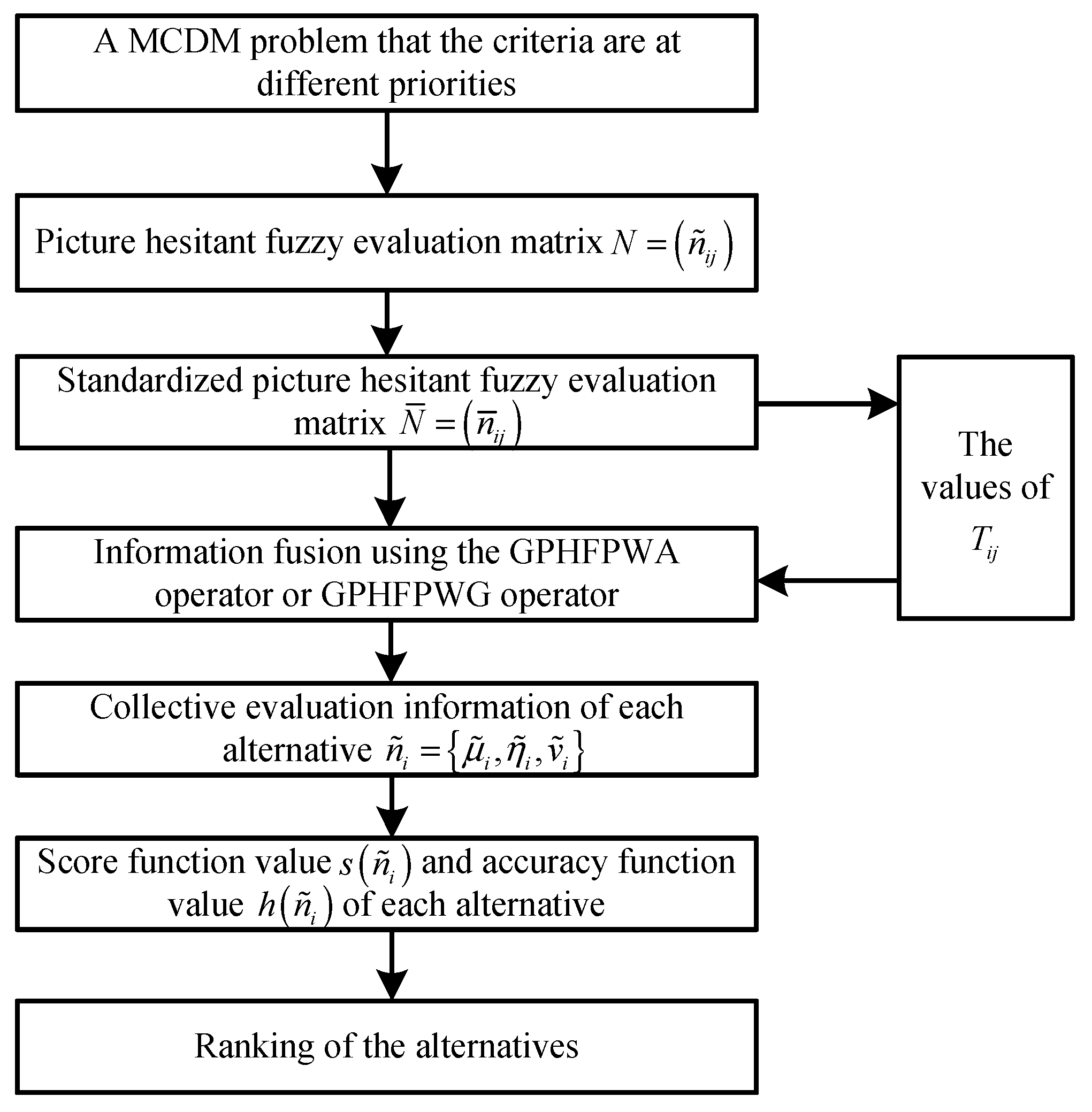
When the criteria are in different priorities, we can solve the MCDM problem combined with the Algorithm 2 based on the GPHFPWA or the GPHFPWG operator. The flow diagram of Algorithm 2 is presented in Figure 2, and the ranking result can be obtained by the following steps.

Algorithm 2. MCDM method based on the GPHFPWA or the GPHFPWG operator.

1: Normalize the PHF evaluation matrix $N$ to obtain the standardized PHF evaluation matrix combined with Equation (51).

2: Compute the values of $T_{ij}$ using the equations as $$T_{ij}={\displaystyle \prod _{k=1}^{j-1}s\left({\tilde{n}}_{ik}\right)},T_{i1}=1.$$ (54)

3: Utilize the GPHFPWA operator $$\begin{gathered} GPHFPW{A}_{\lambda }\left({\overline{n}}_{i1},{\overline{n}}_{i2},\dots ,{\overline{n}}_{in}\right)={\left(\frac{T_{i1}}{{\displaystyle {\sum }_{j=1}^n{T}_{ij}}}{\overline{n}}_{i1}{}^{\lambda }\oplus \frac{T_{i2}}{{\displaystyle {\sum }_{j=1}^n{T}_{ij}}}{\overline{n}}_{i2}{}^{\lambda }\oplus \cdots \oplus \frac{T_{in}}{{\displaystyle {\sum }_{j=1}^n{T}_{ij}}}{\overline{n}}_{in}{}^{\lambda }\right)}^{1/\lambda } \\ ={\displaystyle \underset{{\alpha }_{i1}\in {\tilde{\mu }}_{i1},{\alpha }_{i2}\in {\tilde{\mu }}_{i2},\dots ,{\alpha }_{in}\in {\tilde{\mu }}_{in},{\beta }_{i1}\in {\tilde{\eta }}_{i1},{\beta }_{i2}\in {\tilde{\eta }}_{i2},\dots ,{\beta }_{in}\in {\tilde{\eta }}_{in},{\gamma }_{i1}\in {\tilde{v}}_{i1},{\gamma }_{i2}\in {\tilde{v}}_{i2},\dots ,{\gamma }_{in}\in {\tilde{v}}_{in}}{\cup }\{\left\{{\left(1-{\displaystyle \prod _{j=1}^n{\left(1-{\overline{\alpha }}_{ij}{}^{\lambda }\right)}^{\frac{T_{ij}}{{\displaystyle {\sum }_{j=1}^n{T}_{ij}}}}}\right)}^{1/\lambda }\right\},}\left\{1-{\left(1-{\displaystyle \prod _{j=1}^n{\left(1-{\left(1-{\overline{\beta }}_{ij}\right)}^{\lambda }\right)}^{\frac{T_{ij}}{{\displaystyle {\sum }_{j=1}^n{T}_{ij}}}}}\right)}^{1/\lambda }\right\}, \\ \left\{1-{\left(1-{\displaystyle \prod _{j=1}^n{\left(1-{\left(1-{\overline{\gamma }}_{ij}\right)}^{\lambda }\right)}^{\frac{T_{ij}}{{\displaystyle {\sum }_{j=1}^n{T}_{ij}}}}}\right)}^{1/\lambda }\right\}\} \end{gathered}$$ (55) or the GPHFPWG operator $$\begin{gathered} GPHFPW{G}_{\lambda }\left({\overline{n}}_{i1},{\overline{n}}_{i2},\dots ,{\overline{n}}_{in}\right)=\frac{1}{\lambda }\left({\left(\lambda {\overline{n}}_{i1}\right)}^{\frac{T_{i1}}{{\displaystyle {\sum }_{j=1}^n{T}_{ij}}}}\otimes {\left(\lambda {\overline{n}}_{i2}\right)}^{\frac{T_{i2}}{{\displaystyle {\sum }_{j=1}^n{T}_{ij}}}}\otimes \cdots \otimes {\left(\lambda {\overline{n}}_{in}\right)}^{\frac{T_{in}}{{\displaystyle {\sum }_{j=1}^n{T}_{ij}}}}\right) \\ ={\displaystyle \underset{{\alpha }_{i1}\in {\tilde{\mu }}_{i1},{\alpha }_{i2}\in {\tilde{\mu }}_{i2},\dots ,{\alpha }_{in}\in {\tilde{\mu }}_{in},{\beta }_{i1}\in {\tilde{\eta }}_{i1},{\beta }_{i2}\in {\tilde{\eta }}_{i2},\dots ,{\beta }_{in}\in {\tilde{\eta }}_{in},{\gamma }_{i1}\in {\tilde{v}}_{i1},{\gamma }_{i2}\in {\tilde{v}}_{i2},\dots ,{\gamma }_{in}\in {\tilde{v}}_{in}}{\cup }\{\left\{1-{\left(1-{\displaystyle \prod _{j=1}^n{\left(1-{\left(1-{\overline{\alpha }}_{ij}\right)}^{\lambda }\right)}^{\frac{T_{ij}}{{\displaystyle {\sum }_{j=1}^n{T}_{ij}}}}}\right)}^{1/\lambda }\right\},\left\{{\left(1-{\displaystyle \prod _{j=1}^n{\left(1-{\overline{\beta }}_{ij}{}^{\lambda }\right)}^{\frac{T_{ij}}{{\displaystyle {\sum }_{j=1}^n{T}_{ij}}}}}\right)}^{1/\lambda }\right\},} \\ \left\{{\left(1-{\displaystyle \prod _{j=1}^n{\left(1-{\overline{\gamma }}_{ij}{}^{\lambda }\right)}^{\frac{T_{ij}}{{\displaystyle {\sum }_{j=1}^n{T}_{ij}}}}}\right)}^{1/\lambda }\right\} \end{gathered}$$ (56) to aggregate the standardized PHF evaluation matrix $\overline{N}$ to obtain the collective evaluation information of each alternative, i.e., ${\tilde{n}}_i=\left\{{\tilde{\mu }}_i,{\tilde{\eta }}_i,{\tilde{v}}_i\right\}$.

4: Compute the score and accuracy values of each alternative using Equation (14) and (15).

5: Based on the comparison method of PHFEs, rank the alternatives.

6. Numerical Examples

We adopt two numerical examples of MCDM problems from the study of [25] and [34] and an application of web service selection [37] to show the feasibility and advantages of the proposed methods.

6.1. Implementation

Example 1.

Suppose that an organization wants to construct the enterprise resource planning (ERP) system [25]. After investigating the existing vendors of ERP systems on the market, five potential ERP systems are primary determined to be chosen from, i.e., A_i (i = 1, 2, 3, 4, 5). Decision makers utilize the PHFEs to evaluate the five alternatives with respect to four criteria, namely, function and technology (C₁), strategic fitness (C₂), ability of vendor (C₃), and reputation of vendor (C₄), and the weight vector of the criteria is w = (0.2, 0.1, 0.3, 0.4). Subsequently, the PHF evaluation matrix $N=\left({\tilde{n}}_{ij}\right)$ is obtained as shown in

Table 1. PHF evaluation matrix of Example 1.

Alternatives	${\mathit{C}}_1$	${\mathit{C}}_2$	${\mathit{C}}_3$	${\mathit{C}}_4$
$A_1$	{{0.43,0.53},{0.33}, {0.06,0.09}}	{{0.76,0.89}, {0.05,0.08},{0.03}}	{{0.42},{0.35}, {0.12,0.18}}	{{0.08},{0.75,0.89}, {0.02}}
$A_2$	{{0.53,0.65,0.73}, {0.10,0.12},{0.08}}	{{0.13},{0.53,0.64}, {0.12,0.21}}	{{0.03},{0.77,0.82}, {0.10,0.13}}	{{0.58,0.73},{0.15}, {0.08}}
$A_3$	{{0.72,0.86,0.91}, {0.03},{0.02}}	{{0.07},{0.05,0.09}, {0.05}}	{{0.04},{0.65,0.72,0.85},{0.05,0.10}}	{{0.45,0.68},{0.18,0.26},{0.06}}
$A_4$	{{0.77,0.85},{0.09}, {0.05}}	{{0.65,0.74},{0.10,0.16},{0.10}}	{{0.02},{0.78,0.89},{0.05}}	{{0.08},{0.65,0.84}, {0.06}}
$A_5$	{{0.70,0.81,0.90}, {0.05},{0.02}}	{{0.68},{0.08}, {0.13,0.21}}	{{0.05},{0.77,0.87},{0.06}}	{{0.13},{0.65,0.75}, {0.09}}

.

Then, we can determine the ranking of the five potential ERP systems using the Algorithm 1, which are presented as below.

• Step 1: Because of all the criteria are the benefit type, the standardized PHF evaluation matrix $\overline{N}$ is as same as the PHF evaluation matrix $N$.
• Step 2: Use the GPHFWA ($\lambda =1$) operator to aggregate the standardized PHF evaluation matrix $\overline{N}$, and the collective evaluation information of each alternative is obtained as

  $$\begin{gathered} {\tilde{n}}_1=\{\left\{0.3636,0.3877,0.4113,0.4336\right\},\left\{0.3862,0.4048,0.4136,0.4335\right\},\left\{0.0444,0.0482,0.0502,0.0544\right\}\}; \\ {\tilde{n}}_2=\{\left\{0.4061,0.4401,0.4684,0.5023,0.5308,0.5545\right\},\left\{0.2563,0.2612,0.2612,0.2659,0.2662,0.2709,0.2709,0.2761\right\},\left\{0.0891,0.0942,0.0964,0.1019\right\}\}; \\ {\tilde{n}}_3=\{\left\{0.4014,0.4789,0.5180,0.5230,0.5804,0.6159\right\},\{0.1627,0.1677,0.1725,0.1763,0.1779,0.1870,0.1884,0.1943,0.1999,0.2042,0.2061,0.2166\},\left\{0.0448,0.0551\right\}\}; \\ {\tilde{n}}_4=\{\left\{0.3549,0.3738,0.4077,0.4251\right\},\left\{0.3834,0.3989,0.4018,0.4181,0.4248,0.4420,0.4452,0.5632\right\},\left\{0.0576\right\}\}; \\ {\tilde{n}}_5=\{\left\{0.3468,0.4038,0.4756\right\},\left\{0.3321,0.3444,0.3516,0.3647\right\},\left\{0.0612,0.0642\right\}\}. \end{gathered}$$
• Step 3: Compute the score values of each alternative combined with Equation (14):

  $$s\left({\tilde{n}}_1\right)=0.4701,s\left({\tilde{n}}_2\right)=0.5611,s\left({\tilde{n}}_3\right)=0.6409,s\left({\tilde{n}}_4\right)=0.4553,s\left({\tilde{n}}_5\right)=0.4989.$$
• Step 4: According to the score values, the ranking result of the five ERP systems is determined as $A_3\succ A_2\succ A_5\succ A_1\succ A_4$.

If the GPHFWG operator is utilized in the steps above to complete the information fusion, the ranking procedures are presented as follows.

• Step 1′: See Step 1.
• Step 2′: Use the GPHFWG ($\lambda =1$) operator to aggregate the standardized PHF evaluation matrix $\overline{N}$, and the collective evaluation information of each alternative is obtained as

  $$\begin{gathered} {\tilde{n}}_1=\{\left\{0.2307,0.2343,0.2405,0.2443\right\},\left\{0.5365,0.6663,0.5380,0.6673\right\},\left\{0.0600,0.0797,0.0661,0.0856\right\}\}; \\ {\tilde{n}}_2=\{\left\{0.2017,0.2101,0.2151,0.2212,0.2304,0.2358\right\},\left\{0.4526,0.4550,0.4670,0.4693,0.4914,0.4936,0.5047,0.5070\right\},\left\{0.0901,0.0993,0.0999,0.1090\right\}\}; \\ {\tilde{n}}_3=\{\left\{0.1986,0.2057,0.2081,0.2342,0.2427,0.2454\right\},\{0.3334,0.3363,0.3602,0.3630,0.3766,0.3792,0.4016,0.4042,0.4830,0.4852,0.5038,0.5059\},\left\{0.0481,0.0634\right\}\}; \\ {\tilde{n}}_4=\{\left\{0.1024,0.1037,0.1044,0.1058\right\},\left\{0.5949,0.5977,0.6709,0.6732,0.7038,0.7058,0.7594,0.7611\right\},\left\{0.0591\right\}\}; \\ {\tilde{n}}_5=\{\left\{0.1613,0.1660,0.1696\right\},\left\{0.5850,0.6372,0.6503,0.6943\right\},\left\{0.0716,0.0805\right\}\}. \end{gathered}$$
• Step 3′: Compute the score values of each alternative combined with Equation (14):

  $$s\left({\tilde{n}}_1\right)=0.2813,s\left({\tilde{n}}_2\right)=0.3197,s\left({\tilde{n}}_3\right)=0.3778,s\left({\tilde{n}}_4\right)=0.1808,s\left({\tilde{n}}_5\right)=0.2240.$$
• Step 4′: According to the score values, the ranking result of the five ERP systems is determined as $A_3\succ A_2\succ A_1\succ A_5\succ A_4$.

Example 2.

Suppose a university wants to introduce excellent foreign professors to improve the level of teaching and scientific research [34]. There are five foreign professors who are selected by the University’s human resources department. Based on the priority level, the criteria of investigation is successively morality (C₁), research ability (C₂), teaching capacity (C₃), and educational experience (C₄); a priority relationship $C_1\succ C_2\succ C_3\succ C_4$ exists between the criteria. Then, the PHF evaluation matrix $N=\left({\tilde{n}}_{ij}\right)$ is presented in

Table 2. PHF evaluation matrix in Example 2.

Alternatives	${\mathit{C}}_1$	${\mathit{C}}_2$	${\mathit{C}}_3$	${\mathit{C}}_4$
$A_1$	{{0.40,0.50,0.70},{0.05},{0.10,0.20}}	{{0.65},{0.05,0.08}, {0.15}}	{{0.40,0.50,0.60},{0.03},{0.10,0.20}}	{{0.55},{0.10,0.15}, {0.15}}
$A_2$	{{0.65,0.75},{0.02,0.04},{0.15}}	{{0.60},{0.05,0.10}, {0.10,0.20}}	{{0.75,0.80},{0.06}, {0.05,0.08}}	{{0.40,0.50},{0.20}, {0.15,0.25}}
$A_3$	{{0.70},{0.06,0.10}, {0.10,0.15}}	{{0.20,0.30,0.50},{0.04},{0.30,0.40}}	{{0.50},{0.03,0.06}, {0.30,0.35}}	{{0.50,0.70},{0.10}, {0.10}}
$A_4$	{{0.50,0.60,0.70},{0.08},{0.10}}	{{0.40,0.50},{0.20}, {0.10,0.20}}	{{0.85},{0.03,0.07}, {0.05}}	{{0.45},{0.10,0.20}, {0.15,0.30}}
$A_5$	{{0.65},{0.05,0.10}, {0.15,0.20}}	{{0.50,0.70},{0.08}, {0.20}}	{{0.70,0.80},{0.04}, {0.10}}	{{0.35},{0.10,0.20},{0.30,0.40}}

.

Subsequently, we can determine the ranking of the five foreign professors using the Algorithm 2, which are presented as follows.

• Step 1: Because of all the criteria are the benefit type, the standardized PHF evaluation matrix $\overline{N}$ is as same as the PHF evaluation matrix $N$.
• Step 2: Compute the values of $T_{ij}$ using the Equation (54)

  $$T_{ij}=\left[\begin{array}{cccc}1.000& 0.6667& 0.4783& 0.3157\\ 1.000& 0.7600& 0.5225& 0.4311\\ 1.000& 0.7475& 0.3526& 0.1992\\ 1.000& 0.7100& 0.3905& 0.3417\\ 1.000& 0.7000& 0.4620& 0.3719\end{array}\right].$$
• Step 3: Use the GPHFPWA ($\lambda =1$) operator to aggregate the standardized PHF evaluation matrix $\overline{N}$, and the collective evaluation information of each alternative is obtained as

  $$\begin{gathered} {\tilde{n}}_1=\{\left\{0.5003,0.5177,0.5360,0.5382,0.5522,0.6230,0.6361,0.6516,0.6516\right\},\left\{0.0495,0.0521,0.0562,0.0592\right\},\left\{0.1176,0.1345,0.1558,0.1783\right\}\}; \\ {\tilde{n}}_2=\{\left\{0.6290,0.6396,0.6446,0.6548,0.6723,0.6816,0.6861,0.6950\right\},\left\{0.0460,0.0559,0.0594,0.0722\right\},\left\{0.1084,0.1175,0.1186,0.1287,0.1316,0.1427,0.1441,0.1562\right\}\}; \\ {\tilde{n}}_3=\{\left\{0.5335,0.5533,0.5537,0.5727,0.5996,0.6169\right\},\{0.0494,0.0550,0.0617,0.0686\},\left\{0.1692,0.1732,0.1857,0.1902,0.2018,0.2066,0.2216,0.2269\right\}\}; \\ {\tilde{n}}_4=\{\left\{0.5593,0.5820,0.5978,0.6185,0.6425,0.6609\right\},\left\{0.0921,0.1015,0.1055,0.1162\right\},\left\{0.0947,0.1044,0.1159,0.1277\right\}\}; \\ {\tilde{n}}_5=\{\left\{0.5888,0.6181,0.6429,0.6683\right\},\left\{0.0605,0.0670,0.0796,0.0881\right\},\left\{0.1670,0.1742,0.1871,0.1951\right\}\}. \end{gathered}$$
• Step 4: Compute the score values of each alternative combined with Equation (14)

  $$s\left({\tilde{n}}_1\right)=0.6888,s\left({\tilde{n}}_2\right)=0.7368,s\left({\tilde{n}}_3\right)=0.6580,s\left({\tilde{n}}_4\right)=0.6978,s\left({\tilde{n}}_5\right)=0.6874.$$
• Step 5: According to the score values, the ranking result of the five foreign professors is determined as $A_2\succ A_4\succ A_1\succ A_5\succ A_3$.

If the GPHFPWG operator is utilized in the steps above to complete the information fusion, the ranking procedures are presented as follows.

• Step 1′: See Step 1.
• Step 2′: See Step 2.
• Step 3′: Use the GPHFPWG ($\lambda =1$) operator to aggregate standardized the PHF evaluation matrix $\overline{N}$, and the collective evaluation information of each alternative is obtained as

  $$\begin{gathered} {\tilde{n}}_1=\{\left\{0.4753,0.4963,0.5142,0.5204,0.5434,0.5966,0.6231,0.6455,0.6455\right\},\left\{0.0527,0.0597,0.0609,0.0678\right\},\left\{0.1203,0.1402,0.1614,0.1804\right\}\}; \\ {\tilde{n}}_2=\{\left\{0.6049,0.6124,0.6267,0.6345,0.6376,0.6456,0.6606,0.6689\right\},\left\{0.0668,0.0739,0.0809,0.0878\right\},\left\{0.1176,0.1230,0.1350,0.1403,0.1462,0.1515,0.1630,0.1682\right\}\}; \\ {\tilde{n}}_3=\{\left\{0.4297,0.4424,0.4902,0.5047,0.5788,0.5959\right\},\{0.0526,0.0571,0.0703,0.0748\},\left\{0.2020,0.2110,0.2216,0.2304,0.2410,0.2495,0.2596,0.2680\right\}\}; \\ {\tilde{n}}_4=\{\left\{0.5026,0.5363,0.5416,0.5769,0.5779,0.6155\right\},\left\{0.1119,0.1178,0.1264,0.1322\right\},\left\{0.0994,0.1236,0.1297,0.1531\right\}\}; \\ {\tilde{n}}_5=\{\left\{0.5596,0.5733,0.6141,0.6292\right\},\left\{0.0640,0.0801,0.0838,0.0995\right\},\left\{0.1791,0.1975,0.1985,0.2164\right\}\}. \end{gathered}$$
• Step 4′: Compute the score values of each alternative combined with Equation (14)

  $$s\left({\tilde{n}}_1\right)=0.6757,s\left({\tilde{n}}_2\right)=0.7080,s\left({\tilde{n}}_3\right)=0.6040,s\left({\tilde{n}}_4\right)=0.6550,s\left({\tilde{n}}_5\right)=0.6572.$$
• Step 5′: According to the score values, the ranking result of the five foreign professors is obtained as $A_2\succ A_1\succ A_5\succ A_4\succ A_3$.

6.2. Sensitivity Analysis

To explore the impact of the parameter $\lambda$ on the ranking results, different possible values of $\lambda$ are used in the algorithms of two aforementioned numerical examples, such as 0.001, 0.5, 1, 2, 3, 5, 10, 20, and 50. Then, combined with the proposed methods, the different rankings of alternatives are presented in

Table 3. Sensitivity analysis results obtained by the GPHFWA operator.

Values	$\mathit{s}\left({\tilde{\mathit{n}}}_1\right)$	$\mathit{s}\left({\tilde{\mathit{n}}}_2\right)$	$\mathit{s}\left({\tilde{\mathit{n}}}_3\right)$	$\mathit{s}\left({\tilde{\mathit{n}}}_4\right)$	$\mathit{s}\left({\tilde{\mathit{n}}}_5\right)$	Ranking
$\lambda =0.001$	0.4117	0.4988	0.5787	0.3388	0.4058	$A_3\succ A_2\succ A_1\succ A_5\succ A_4$
$\lambda =0.5$	0.4412	0.5328	0.6124	0.3977	0.4526	$A_3\succ A_2\succ A_5\succ A_1\succ A_4$
$\lambda =1$	0.4701	0.5611	0.6409	0.4553	0.4989	$A_3\succ A_2\succ A_5\succ A_1\succ A_4$
$\lambda =2$	0.5197	0.6001	0.6812	0.5426	0.5743	$A_3\succ A_2\succ A_5\succ A_4\succ A_1$
$\lambda =3$	0.5578	0.6242	0.7074	0.5981	0.6255	$A_3\succ A_5\succ A_2\succ A_4\succ A_1$
$\lambda =5$	0.6133	0.6522	0.7406	0.6613	0.6852	$A_3\succ A_5\succ A_4\succ A_2\succ A_1$
$\lambda =10$	0.6965	0.6831	0.7837	0.7274	0.7481	$A_3\succ A_5\succ A_4\succ A_1\succ A_2$
$\lambda =20$	0.7679	0.7062	0.8197	0.7722	0.7916	$A_3\succ A_5\succ A_4\succ A_1\succ A_2$
$\lambda =50$	0.8243	0.7274	0.8527	0.8063	0.8280	$A_3\succ A_5\succ A_1\succ A_4\succ A_2$

,

Table 4. Sensitivity analysis results obtained by the GPHFWG operator.

Values	$\mathit{s}\left({\tilde{\mathit{n}}}_1\right)$	$\mathit{s}\left({\tilde{\mathit{n}}}_2\right)$	$\mathit{s}\left({\tilde{\mathit{n}}}_3\right)$	$\mathit{s}\left({\tilde{\mathit{n}}}_4\right)$	$\mathit{s}\left({\tilde{\mathit{n}}}_5\right)$	Ranking
$\lambda =0.001$	0.3227	0.3791	0.4486	0.2142	0.2720	$A_3\succ A_2\succ A_1\succ A_5\succ A_4$
$\lambda =0.5$	0.3019	0.3492	0.4120	0.1960	0.2457	$A_3\succ A_2\succ A_1\succ A_5\succ A_4$
$\lambda =1$	0.2813	0.3197	0.3778	0.1808	0.2240	$A_3\succ A_2\succ A_1\succ A_5\succ A_4$
$\lambda =2$	0.2451	0.2690	0.3237	0.1587	0.1926	$A_3\succ A_2\succ A_1\succ A_5\succ A_4$
$\lambda =3$	0.2168	0.2314	0.2858	0.1439	0.1716	$A_3\succ A_2\succ A_1\succ A_5\succ A_4$
$\lambda =5$	0.1780	0.1829	0.2389	0.1249	0.1441	$A_3\succ A_2\succ A_1\succ A_5\succ A_4$
$\lambda =10$	0.1301	0.1265	0.1878	0.0991	0.1093	$A_3\succ A_1\succ A_2\succ A_5\succ A_4$
$\lambda =20$	0.1252	0.1158	0.1923	0.1216	0.1095	$A_3\succ A_1\succ A_4\succ A_2\succ A_5$
$\lambda =50$	0.1458	0.1377	0.1692	0.1041	0.1351	$A_3\succ A_1\succ A_2\succ A_5\succ A_4$

,

Table 5. Sensitivity analysis results obtained by the GPHFPWA operator.

Values	$\mathit{s}\left({\tilde{\mathit{n}}}_1\right)$	$\mathit{s}\left({\tilde{\mathit{n}}}_2\right)$	$\mathit{s}\left({\tilde{\mathit{n}}}_3\right)$	$\mathit{s}\left({\tilde{\mathit{n}}}_4\right)$	$\mathit{s}\left({\tilde{\mathit{n}}}_5\right)$	Ranking
$\lambda =0.001$	0.6866	0.7337	0.6477	0.6911	0.6829	$A_2\succ A_4\succ A_1\succ A_5\succ A_3$
$\lambda =0.5$	0.6877	0.7352	0.6529	0.6944	0.6852	$A_2\succ A_4\succ A_1\succ A_5\succ A_3$
$\lambda =1$	0.6888	0.7368	0.6580	0.6978	0.6874	$A_2\succ A_4\succ A_1\succ A_5\succ A_3$
$\lambda =2$	0.6913	0.7399	0.6680	0.7054	0.6920	$A_2\succ A_4\succ A_5\succ A_1\succ A_3$
$\lambda =3$	0.6940	0.7432	0.6769	0.7135	0.6964	$A_2\succ A_4\succ A_5\succ A_1\succ A_3$
$\lambda =5$	0.6994	0.7495	0.6915	0.7298	0.7045	$A_2\succ A_4\succ A_5\succ A_1\succ A_3$
$\lambda =10$	0.7108	0.7634	0.7151	0.7628	0.7203	$A_2\succ A_4\succ A_5\succ A_3\succ A_1$
$\lambda =20$	0.7243	0.7831	0.7369	0.7976	0.7407	$A_4\succ A_2\succ A_5\succ A_3\succ A_1$
$\lambda =50$	0.7408	0.8092	0.7570	0.8332	0.7693	$A_4\succ A_2\succ A_5\succ A_3\succ A_1$

and

Table 6. Sensitivity analysis results obtained by the GPHFPWG operator.

Values	$\mathit{s}\left({\tilde{\mathit{n}}}_1\right)$	$\mathit{s}\left({\tilde{\mathit{n}}}_2\right)$	$\mathit{s}\left({\tilde{\mathit{n}}}_3\right)$	$\mathit{s}\left({\tilde{\mathit{n}}}_4\right)$	$\mathit{s}\left({\tilde{\mathit{n}}}_5\right)$	Ranking
$\lambda =0.001$	0.6814	0.7230	0.6242	0.6733	0.6706	$A_2\succ A_1\succ A_4\succ A_5\succ A_3$
$\lambda =0.5$	0.6789	0.7163	0.6147	0.6647	0.6646	$A_2\succ A_1\succ A_4\succ A_5\succ A_3$
$\lambda =1$	0.6757	0.7080	0.6040	0.6550	0.6572	$A_2\succ A_1\succ A_5\succ A_4\succ A_3$
$\lambda =2$	0.6680	0.6885	0.5815	0.6344	0.6393	$A_2\succ A_1\succ A_5\succ A_4\succ A_3$
$\lambda =3$	0.6597	0.6692	0.5611	0.6155	0.6194	$A_2\succ A_1\succ A_5\succ A_4\succ A_3$
$\lambda =5$	0.6442	0.6378	0.5306	0.5873	0.5815	$A_1\succ A_2\succ A_4\succ A_5\succ A_3$
$\lambda =10$	0.6190	0.5931	0.4921	0.5524	0.5213	$A_1\succ A_2\succ A_4\succ A_5\succ A_3$
$\lambda =20$	0.6727	0.5774	0.5122	0.5451	0.5002	$A_1\succ A_2\succ A_4\succ A_3\succ A_5$
$\lambda =50$	0.7825	0.7355	0.6732	0.7214	0.6872	$A_1\succ A_2\succ A_4\succ A_5\succ A_3$

. From Table 3 and Table 4, we can find that the best potential ERP system in Example 1 is always $A_3$ using both the GPHFWA operator and GPHFWG operator; however, some differences exist between the ranking results concerning different values of $\lambda$. Table 5 and Table 6 show that when we utilize the GPHFPWA operator to complete the information fusion, the best foreign professor is $A_2$ for $0.001\le \lambda \le 10$, but the best alternative is $A_4$ for $20\le \lambda \le 50$. In addition, when the GPHFPWG operator is used in Algorithm 2, the best foreign professor is $A_2$ for $0.001\le \lambda \le 3$, but the best alternative is $A_1$ for $5\le \lambda \le 50$. On the other hand, the score values of all the alternatives vary with different values of $\lambda$; the reason is that the aggregation processes of the proposed operators have changed. For instance, when $\lambda =2$, the GPHFWA operator can be reduced to the picture hesitant fuzzy weighted quadratic averaging (PHFWQA) operator as

$$PHFWQA\left({\overline{n}}_{i1},{\overline{n}}_{i2},\dots ,{\overline{n}}_{in}\right)={\left(w_1{\overline{n}}_{i1}{}^2\oplus w_2{\overline{n}}_{i2}{}^2\oplus \cdots \oplus w_n{\overline{n}}_{in}{}^2\right)}^{1/2}.$$

when $\lambda =3$, the GPHFWA operator can be reduced to the picture hesitant fuzzy weighted cubic averaging (PHFWCA) operator as

$$PHFWCA\left({\overline{n}}_{i1},{\overline{n}}_{i2},\dots ,{\overline{n}}_{in}\right)={\left(w_1{\overline{n}}_{i1}{}^3\oplus w_2{\overline{n}}_{i2}{}^3\oplus \cdots \oplus w_n{\overline{n}}_{in}{}^3\right)}^{1/3}.$$

Besides, the following results can be obtained from Table 3, Table 4, Table 5 and Table 6:

(1)

In Example 1, the score values of each alternative obtained by the GPHFWA operator are bigger than those obtained by the GPHFWG operator, and the difference between them increases along with the increasing of $\lambda$. It means that the GPHFWA operator is more suitable to aggregate the PHFEs of optimistic decision makers, while the GPHFWG operator can reflect the opinion of pessimistic decision makers. Furthermore, the level of optimism and pessimism are greater with the bigger value of $\lambda$.

(2)

In Example 2, the score values of each alternative obtained by the GPHFPWA and GPHFPWG operators are relatively stable when the different values of $\lambda$ are used; the parameter $\lambda$ cannot reflect the attitude of decision makers. In addition, the best alternative varies when the value of $\lambda$ is relatively high, while the best alternative is always the same in Example 1. It means that the rankings obtained by the GPHFPWA and GPHFPWG operators are more affected by the parameter $\lambda$ than those obtained by the GPHFWA and GPHFWG operators.

The aforementioned sensitivity analysis results show that the value of $\lambda$ plays a very important role in MCDM problems, especially when the value of $\lambda$ is relatively high. The value of $\lambda$ can be determined based on the personal preference of decision makers to obtain different ranking results; thus, the proposed methods are highly flexible to deal with different situations in practice.

6.3. Comparative Analysis

To prove the feasibility of the proposed MCDM methods, the rankings of Example 1 in this paper are compared with the rankings obtained by the existing MCDM methods as presented in

Table 7. Comparison result of Example 1.

MCDM method	Ranking
The GPHFWA operator ($\lambda =1$)	$A_3\succ A_2\succ A_5\succ A_1\succ A_4$
The GPHFWG operator ($\lambda =1$)	$A_3\succ A_2\succ A_1\succ A_5\succ A_4$
The PFWA operator	$A_3\succ A_2\succ A_1\succ A_5\succ A_4$
The PFWG operator	$A_3\succ A_1\succ A_2\succ A_5\succ A_4$
The picture fuzzy cross-entropy method	$A_3\succ A_1\succ A_2\succ A_5\succ A_4$

; including the PFWA and PFWG operators [25], and the picture fuzzy cross-entropy method [16]. Similarly, a comparison of Example 2 between the GPHFPWA and GPHFPWG operators and the HFPWA and HFPWG operators [34] is presented in

Table 8. Comparison result of Example 2.

MCDM method	Ranking
The GPHFPWA operator ($\lambda =1$)	$A_2\succ A_4\succ A_1\succ A_5\succ A_3$
The GPHFPWG operator ($\lambda =1$)	$A_2\succ A_1\succ A_5\succ A_4\succ A_3$
The HFPWA operator	$A_5\succ A_2\succ A_1\succ A_4\succ A_3$
The HFPWG operator	$A_2\succ A_5\succ A_1\succ A_4\succ A_3$

.

Table 7 shows that the best alternative of Example 2 obtained by the MCDM methods based on the GPHFWA and GPHFWG operators is always $A_3$, which is consistent with the existing methods; the results can demonstrate the feasibility of the proposed method. Compared with the PFS that is used in the study of [25] and [16], PHFS proposed in this paper can convey the human opinions more effectively, including yes, abstain, no, and refusal. For instance, the evaluation information of the alternative $A_1$ concerning the criteria $C_1$ that are given by decision maker is expressed as a PFN (0.53,0.33,0.09) [16,25]. In practice, decision maker may feel doubtful to determine an exact value of each membership level. Obviously, PFS cannot deal with this situation; however, we can use PHFS to represent the evaluation information as a PHFE {{0.43,0.53}, {0.33}, {0.06,0.09}} as shown in Table 1. Consequently, the proposed method can solve the MCDM problems when decision makers feel difficulty to determine the accurate value of each membership level. On the other hand, when the numbers of the criteria are relatively large, the aggregation process of the proposed operators will be more complicated than the existing methods and the data size will be relatively large; it is the limitation of the proposed method. Table 8 shows that the best alternative of Example 2 obtained by the HFPWA operator is $A_5$, but the result of other MCDM methods is $A_2$. The main reason of the difference is that the MCDM methods combined with the HFPWA and HFPWG operators ignore some complex evaluation information of decision makers in practice. UTHFS allows the decision makers to give several values of positive membership level, for instance, the evaluation information of the alternative $A_1$ concerning the criteria $C_1$ that are given by decision maker is expressed as a UTHFE (0.4,0.5,0.7) [34]. Nevertheless, in some particular situations, it is not convincing to express the evaluation information that only considers the positive membership level of decision makers; many scholars have focused on this problem and made some improvements to UTHFS [10,19]. Thus, we can overcome the limitation of UTHFS combined with the proposed method. It is worth noting that the GPHFPWA and GPHFPWG operators also have the same disadvantage as the GPHFWA and GPHFWG operators.

According to the aforementioned comparison results, we can summarize the advantages and disadvantages of the different MCDM methods (see

Table 9. Comparison of each MCDM methods.

Methods	Advantages	Disadvantages
The GPHFWA/GPHFWG operator	• The human opinions including yes, abstain, no, and refusal can be expressed, and each membership functions can be represented by several possible values. • The operators can be reduced to other forms by varying the value of $\lambda$. • The PHFS can be transformed into its special cases, i.e., FS, IFS, PFS, and UTHFS.	• The calculating process is complex when the numbers of criteria are relatively large. • The size of data is relatively large.
The PFWA/PFWG operator	• The human opinions including yes, abstain, no, and refusal can be expressed. • The PFS can be transformed into IFS and FS.	• It cannot express the evaluation information when decision makers have difficulty determining an accurate value of each membership level.
Picture fuzzy cross-entropy	• The human opinions including yes, abstain, no, and refusal can be expressed. • The PFS can be transformed into IFS and FS. • The ranking is obtained without aggregating the evaluation information; it can avoid the loss of information. • The step of normalizing the evaluation information can be omitted.	• It cannot express the evaluation information when decision makers have difficulty determining an accurate value of each membership level. • It cannot solve the multiple criteria group decision-making problems.
The GPHFPWA/GPHFPWG operator	• The human opinions including yes, abstain, no, and refusal can be expressed, and each membership functions can be represented by several possible values. • The operators can be reduced to other forms by varying the value of the $\lambda$. • The PHFS can be transformed into its special cases, i.e., FS, IFS, PFS, and UTHFS. • It can solve the MCDM problem that the criteria are in different priorities.	• The calculating process is complex when the numbers of criteria are relatively large. • The size of data is relatively large.
The HFPWA/HFPWG operator	• The positive membership function can be expressed by several possible values. • It can solve the MCDM problem that the criteria are in different priorities.	• It cannot express the human opinions including abstain, no, and refusal.

), as well as their respective fields of application (see

Table 10. MCDM application fields of each MCDM method.

Methods	MCDM Application Fields
The GPHFWA/GPHFWG operator	• The evaluation information of decision makers is diverse. • Decision makers feel doubtful to determine the accurate value of each membership level. • The numbers of the criteria are relatively small.
The PFWA/PFWG operator	• The evaluation information of decision makers is diverse.
Picture fuzzy cross entropy	• The evaluation information of decision maker is diverse. • The alternatives are evaluated by an individual decision maker.
The GPHFPWA/GPHFPWG operator	• The evaluation information of decision makers is diverse. • Decision makers feel doubtful to determine the accurate value of each membership level. • The numbers of the criteria are relatively small. • The criteria are in different priorities.
The HFPWA/HFPWG operator	• Decision makers feel doubtful to determine the accurate value of positive membership level. • The criteria are in different priorities.

). In addition, the benefits of the aggregation process by using the proposed operators are presented as in the following.

(1) The Expansion of the Evaluation Information

The GPHFWA, GPHFWG, GPHFPWA, and GPHFPWG operators can solve the MCDM problems under PHF environment. PHFS proposed in this paper can express the different human opinions in real life and allow the decision makers to give several possible values of the different membership levels; thus, it can simultaneously depict the uncertainty and hesitancy of decision makers’ evaluation information, which cannot be achieved by PFS and UTHFS. Therefore, when decision makers are not fully aware of the evaluation target and feel doubtful about each membership level, it is reasonable to deal with these MCDM problems combined with the proposed methods. Furthermore, as a generalized form of FS, IFS, PFS, and UTHFS, we can transform the proposed methods into the existing MCDM methods if necessary.

(2) The Flexibility of Information Aggregation with Different Values of $\lambda$

Recall the sensitivity analysis in Section 6.2, the proposed operators can be reduced to other specific PHF aggregation operators by varying the value of $\lambda$; thus, the proposed methods are highly flexible to deal with different situations. Furthermore, the parameter $\lambda$ can also be regarded as a measure of the optimism and pessimism level of decision makers in the information fusion of the GPHFWA and GPHFWG operators; and the value of $\lambda$ can be determined by decision makers according to their preferences in practice.

(3) The Simplicity of Dealing with Different Types of Criteria

During the MCDM process, the weight values of criteria play an important role and will affect the final ranking results. The criteria can be divided into two categories: one is in the same priority, the other is in different priorities. On the one hand, when the criteria have the same priority level, we can utilize the proposed method based on the GPHFWA and GPHFWG operators combined with the weight vector of criteria to solve the MCDM problem. On the other hand, when the criteria have different priority levels, the GPHFPWA and GPHFPWG operators can be introduced to determine the ranking of alternatives. In practice, we can use different aggregation operators in this paper to deal with different situations.

6.4. Application of Web Service Selection

To investigate the applications of the proposed methods in a more realistic scenario, we use the proposed methods to solve the Quality of Service (QoS) based web service selection problem [37]. According to the study of [37], the evaluation information of QoS is measured by a crisp number scale of 1–9, and the related criteria are availability ($C_1$), throughput ($C_2$), successability ($C_3$), reliability ($C_4$), compliance ($C_5$), best practices ($C_6$), documentation ($C_7$), latency ($C_8$), and response time ($C_9$). Due to the criteria latency and response time are the cost type criteria, the closer the evaluation values concerning these two criteria are to 1, the better the alternative.

Suppose there are 20 web services to be evaluated concerning the aforementioned nine criteria, i.e., $W{S}_i\left(i=1,2,\dots ,20\right)$; the evaluation information of each web service is presented in

Table 11. Evaluation information of each web service.

Alternatives	${\mathit{C}}_1$	${\mathit{C}}_2$	${\mathit{C}}_3$	${\mathit{C}}_4$	${\mathit{C}}_5$	${\mathit{C}}_6$	${\mathit{C}}_7$	${\mathit{C}}_8$	${\mathit{C}}_9$
$W{S}_1$	3	4	2	5	6	7	6	2	8
$W{S}_2$	4	5	2	3	4	6	8	3	4
$W{S}_3$	3	5	6	8	3	2	2	4	5
$W{S}_4$	4	4	5	5	6	2	6	7	8
$W{S}_5$	5	6	2	4	7	7	8	8	3
$W{S}_6$	4	4	3	7	6	8	6	8	6
$W{S}_7$	4	4	5	7	8	7	7	4	3
$W{S}_8$	6	7	6	6	5	7	8	6	3
$W{S}_9$	5	3	2	2	6	5	2	4	7
$W{S}_{10}$	8	8	7	6	2	2	3	4	3
$W{S}_{11}$	5	8	4	4	5	7	4	5	8
$W{S}_{12}$	4	5	5	5	6	8	7	6	6
$W{S}_{13}$	6	4	7	6	4	5	4	4	5
$W{S}_{14}$	4	6	5	4	5	4	6	7	4
$W{S}_{15}$	7	5	6	2	7	6	5	5	2
$W{S}_{16}$	3	6	4	7	2	3	8	2	4
$W{S}_{17}$	4	4	8	4	4	5	2	4	8
$W{S}_{18}$	4	3	5	3	5	4	4	6	6
$W{S}_{19}$	5	4	4	6	6	7	6	7	2
$W{S}_{20}$	6	2	3	5	4	6	5	5	5

. As each evaluation value in [37] is expressed by an exact crisp number, the PHFS can be reduced to the PFS to represent the evaluation information of each web service. Based on the relationship between the linguistic variables and IFNs [38], we develop the transformation relationship between the linguistic variables and PFNs as presented in

Table 12. Transformation between linguistic variables and PFNs.

Crisp numbers	Linguistic variables	PFNs
1	Extremely low (EL)	(0.05,0.05,0.85)
2	Very low (VL)	(0.15,0.05,0.75)
3	Low (L)	(0.25,0.05,0.65)
4	Medium low (ML)	(0.35,0.05,0.55)
5	Medium (M)	(0.45,0.05,0.45)
6	Medium high (MH)	(0.55,0.05,0.35)
7	High (H)	(0.65,0.05,0.25)
8	Very high (VH)	(0.75,0.05,0.15)
9	Extremely high (EH)	(0.85,0.05,0.05)

. Then, the evaluation information in Table 11 can be transformed into a PF evaluation matrix $A=\left(a_{ij}\right)\left(i=1,2,\dots ,20; j=1,2,\dots ,9\right)$, and the ranking of the 20 web services can be obtained by the Algorithm 1 in this paper. Subsequently, the ranking result will be compared with the rankings determined by AHP, TOPSIS, COPRAS, VIKOR, and SAW methods in [37]. It is worth noting that, in order to compare different MCDM methods, more effectively we suppose each criteria is considered equally important, i.e., $w_j=1/9\left(j=1,2,\dots ,9\right)$. Then, the ranking of the 20 web services can be determined by the following steps.

• Step 1: According to the Definition 3, normalize the PF evaluation matrix $A=\left(a_{ij}\right)$ to the standardized PF evaluation matrix $\overline{A}=\left({\overline{a}}_{ij}\right)$ as

  $${\overline{a}}_{ij}=\{\begin{array}{ll}{a}_{ij},& \mathrm{for}\mathrm{the}\mathrm{benefit}\mathrm{criteria};\\ {\left(a_{ij}\right)}^c,& \mathrm{for}\mathrm{the}\mathrm{cost}\mathrm{criteria}.\end{array}$$

  (57)
• Step 2: Utilize the GPFWA ($\lambda =1$) operator

  $$GPFW{A}_{\lambda =1}\left({\overline{a}}_{i1},{\overline{a}}_{i2},\dots ,{\overline{a}}_{i9}\right)=a_i=\left(1-{\displaystyle \prod _{j=1}^9{\left(1-{\overline{\mu }}_{ij}\right)}^{w_j}},{\displaystyle \prod _{j=1}^9{\left({\overline{\eta }}_{ij}\right)}^{w_j}},{\displaystyle \prod _{j=1}^9{\left({\overline{v}}_{ij}\right)}^{w_j}}\right)$$

  to aggregated the PF evaluation matrix $\overline{A}=\left({\overline{a}}_{ij}\right)$, and the collective PFNs of each web service are obtained.
• Step 3: Compute the score values of each web service using the equation

  $$s\left(a_i\right)=\left(1+{\mu }_i-{\eta }_i-v_i\right)/2.$$

  (58)

Then, the ranking of the 20 web services can be determined; the lager the score value, the better the web service. The related data of the ranking are presented in

Table 13. Ranking results obtained by the proposed method.

Alternatives	Collective Evaluation Information	Score Values	Ranking
$W{S}_1$	(0.4677,0.0500,0.4210)	0.4983	12
$W{S}_2$	(0.4833,0.0500,0.4068)	0.5133	9
$W{S}_3$	(0.4313,0.0500,0.4579)	0.4617	15
$W{S}_4$	(0.3776,0.0500,0.5192)	0.4042	18
$W{S}_5$	(0.5244,0.0500,0.3647)	0.5548	5
$W{S}_6$	(0.4736,0.0500,0.4159)	0.5038	11
$W{S}_7$	(0.5817,0.0500,0.3119)	0.6099	2
$W{S}_8$	(0.5871,0.0500,0.3079)	0.6146	1
$W{S}_9$	(0.3485,0.0500,0.5475)	0.3755	20
$W{S}_{10}$	(0.5447,0.0500,0.3414)	0.5767	3
$W{S}_{11}$	(0.4683,0.0500,0.4222)	0.4980	13
$W{S}_{12}$	(0.5045,0.0500,0.3879)	0.5333	8
$W{S}_{13}$	(0.4828,0.0500,0.4145)	0.5091	10
$W{S}_{14}$	(0.4371,0.0500,0.4609)	0.4631	14
$W{S}_{15}$	(0.5426,0.0500,0.3498)	0.5714	4
$W{S}_{16}$	(0.5191,0.0500,0.3668)	0.5511	6
$W{S}_{17}$	(0.4154,0.0500,0.4744)	0.4455	16
$W{S}_{18}$	(0.3535,0.0500,0.5459)	0.3788	19
$W{S}_{19}$	(0.5186,0.0500,0.3737)	0.5474	7
$W{S}_{20}$	(0.4179,0.0500,0.4798)	0.4440	17

.

To verify the accuracy of the ranking obtained by the proposed method, we use AHP, TOPSIS, COPRAS, VIKOR, and SAW methods to solve the web service selection problem combined with the evaluation information in Table 11. Subsequently, the ranking results of different MCDM methods are presented in

Table 14. Ranking of web services of different MCDM methods.

Alternatives	The Proposed Method	AHP	TOPSIS	COPRAS	VIKOR	SAW
$W{S}_1$	12	13	14	12	15	14
$W{S}_2$	9	10	11	6	12	12
$W{S}_3$	15	16	15	11	17	19
$W{S}_4$	18	18	18	20	19	18
$W{S}_5$	5	6	8	9	9	9
$W{S}_6$	11	11	12	16	14	13
$W{S}_7$	2	2	2	1	3	2
$W{S}_8$	1	1	1	5	1	1
$W{S}_9$	20	20	20	19	20	20
$W{S}_{10}$	3	4	4	4	8	10
$W{S}_{11}$	13	11	10	15	13	8
$W{S}_{12}$	8	6	7	10	4	6
$W{S}_{13}$	10	8	6	8	2	5
$W{S}_{14}$	14	13	13	13	6	7
$W{S}_{15}$	4	3	3	3	7	3
$W{S}_{16}$	6	8	9	2	11	11
$W{S}_{17}$	16	17	16	17	18	16
$W{S}_{18}$	19	19	19	18	10	17
$W{S}_{19}$	7	4	5	7	5	4
$W{S}_{20}$	17	15	17	14	16	15

. The Spearman’s rank correlation coefficient is a powerful tool for measuring the similarity between two MCDM methods [39]. Then, we can calculate the Spearman’s rank correlation coefficients between the proposed method and the other five MCDM methods as shown in

Table 15. Spearman’s rank correlation coefficients between the proposed method and the other MCDM methods.

Existing MCDM Methods	Spearman’s Rank Correlation Coefficients
AHP	0.9722
TOPSIS	0.9549
COPRAS	0.9023
VIKOR	0.7429
SAW	0.8165

. Table 15 shows that the Spearman’s rank correlation coefficients between the proposed method and AHP and TOPSIS are 0.9722 and 0.9549, respectively, which demonstrate that the proposed method is highly correlated with these two methods. AHP and TOPSIS methods have been approved to be the most suitable two methods to solve web service selection problems [39]; thus, the comparison results above illustrate the feasibility of the proposed method.

From the information aggregation of the proposed method, we can find that the calculating procedure of the proposed method is more complicated than AHP and TOPSIS methods. In addition, TOPSIS method does not require the transformation of the evaluation information concerning cost and benefit type criteria. However, when decision makers are not sure if it is 3 or 4 about the evaluation information of the web service $W{S}_1$ concerning the criteria $C_1$, AHP and TOPSIS methods cannot deal with this situation in practice; we can use PHFS to express the evaluation information above, i.e., {{0.25,0.35},{0.05},{0.55,0.65}}. On the other hand, when the criteria are in different priorities, the GPHFPWA and GPHFPWG operators can be used to aggregation the evaluation information. Thus, the AHP, TOPSIS, and proposed methods have their own advantages and disadvantages; in real life, decision makers can determine to utilize which MCDM methods to solve problems according to the actual situations.

7. Conclusions

Combined with the picture fuzzy set and uniformly typical hesitant fuzzy set, this paper develops the picture hesitant fuzzy set, in which the positive, neutral, negative, and refusal membership degrees are expressed by several possible values. Then, the operations and comparison method of picture hesitant fuzzy elements are developed. To solve the multiple criteria decision-making problems under picture hesitant fuzzy environment, the generalized picture hesitant fuzzy weighted averaging and generalized picture hesitant fuzzy weighted geometric operators are put forward to aggregate the picture hesitant elements given by decision maker. Furthermore, considering the different priorities between the related criteria in practice, the generalized picture hesitant fuzzy prioritized weighted averaging and generalized picture hesitant fuzzy prioritized weighted geometric operators are proposed. Meanwhile, some desirable properties and the reduced operators of them are investigated in detail. Finally, two kinds of multiple criteria decision-making methods combined with the proposed operators are constructed to solve the multiple criteria decision-making problems in different situations. Subsequently, two numerical examples and an application of web service selection are provided to indicate the applications and advantages of the proposed methods.

In future research, we will investigate other operations of picture hesitant fuzzy elements and develop different aggregation operators to aggregate picture hesitant fuzzy elements. In addition, we will propose the consensus model to improve the proposed methods; then, the non-consensus evaluation information of decision makers will be revised to obtain a more accurate ranking result.

References

- Mardani, A.; Jusoh, A.; Zavadskas, E.K. Fuzzy multiple criteria decision-making techniques and applications–two decades review from 1994 to 2014. Expert Syst. Appl. 2015, 42, 4126–4148. [Google Scholar] [CrossRef]
- Morente-Molinera, J.A.; Kou, G.; González-Crespo, R.; Corchado, J.M.; Herrera-Viedma, E. Solving multi-criteria group decision making problems under environments with a high number of alternatives using fuzzy ontologies and multi-granular linguistic modelling methods. Knowl. Syst. 2017, 137, 54–64. [Google Scholar] [CrossRef]
- Hernández, F.L.; Ory, E.G.D.; Aguilar, S.R.; González-Crespo, R. Residue properties for the arithmetical estimation of the image quantization table. Appl. Soft Comput. 2018, 67, 309–321. [Google Scholar] [CrossRef]
- Zadeh, L.A. Fuzzy sets. Inf. Control 1965, 8, 338–353. [Google Scholar] [CrossRef] [Green Version]
- Atanassov, K.T. Intuitionistic fuzzy sets. Fuzzy sets Syst. 1986, 20, 87–96. [Google Scholar] [CrossRef]
- Atanassov, K.T. Gargov, G. Interval valued intuitionistic fuzzy sets. Fuzzy Sets Syst. 1989, 31, 343–349. [Google Scholar] [CrossRef]
- Cường, B.C. Picture fuzzy sets. J. Comput. Sci.Cybern. 2015, 30, 409–420. [Google Scholar] [CrossRef]
- Torra, V. Hesitant fuzzy sets. Int. J. Intell. Syst. 2010, 25, 529–539. [Google Scholar] [CrossRef]
- Ye, J. Trapezoidal neutrosophic set and its application to multiple attribute decision-making. Neural Comput. Appl. 2015, 26, 1157–1166. [Google Scholar] [CrossRef]
- Zhu, B.; Xu, Z.S.; Xia, M.M. Dual hesitant fuzzy sets. J. Appl. Math. 2012, 2012, 2607–2645. [Google Scholar] [CrossRef]
- Liu, F.; Yuan, X.H. Fuzzy number intuitionistic fuzzy set. Fuzzy Syst. Math. 2007, 21, 88–91. [Google Scholar]
- Garg, H. Some picture fuzzy aggregation operators and their applications to multicriteria decision-making. Arab. J. Sci. Eng. 2017, 42, 1–16. [Google Scholar] [CrossRef]
- Cuong, B. Picture fuzzy sets-first results. Part 1. In Proceedings of the Third World Congress on Information and Communication WICT’2013, Hanoi, Vietnam, 15–18 December 2013; pp. 1–6. [Google Scholar]
- Singh, P. Correlation coefficients for picture fuzzy sets. J. Intell. Fuzzy Syst. 2015, 28, 1–12. [Google Scholar]
- Son, L.H. Generalized picture distance measure and applications to picture fuzzy clustering. Appl. Soft Comput. 2016, 46, 284–295. [Google Scholar] [CrossRef]
- Wei, G.W. Picture fuzzy cross-entropy for multiple attribute decision making problems. J. Bus. Econ. Manag. 2016, 17, 491–502. [Google Scholar] [CrossRef]
- Torra, V.; Narukawa, Y. On hesitant fuzzy sets and decision. In Proceedings of the IEEE International Conference on Fuzzy Systems, Jeju Island, Korea, 20–24 August 2009; pp. 1378–1382. [Google Scholar]
- Chen, N.; Xu, Z.S.; Xia, M.M. Interval-valued hesitant preference relations and their applications to group decision making. Knowl. Syst. 2013, 37, 528–540. [Google Scholar] [CrossRef]
- Farhadinia, B. Correlation for dual hesitant fuzzy sets and dual interval-valued hesitant fuzzy sets. Int. J. Intell. Syst. 2013, 29, 184–205. [Google Scholar] [CrossRef]
- Xu, Z.S.; Yager, R.R. Some geometric aggregation operators based on intuitionistic fuzzy sets. Int. J. Intell. Syst. 2006, 35, 417–433. [Google Scholar] [CrossRef]
- Xu, Z.S. Intuitionistic fuzzy aggregation operators. IEEE Trans. Fuzzy Syst. 2007, 15, 1179–1187. [Google Scholar]
- Xu, Z.S. Methods for aggregating interval-valued intuitionistic fuzzy information and their application to decision making. Control Decis. 2007, 22, 215–219. [Google Scholar]
- Xu, Z.S.; Chen, J. Approach to group decision making based on interval-valued intuitionistic judgment matrices. Syst. Eng. Theory Pract. 2007, 27, 126–133. [Google Scholar] [CrossRef]
- Xu, Z.S.; Chen, J. On geometric aggregation over interval-valued intuitionistic fuzzy information. In Proceedings of the International Conference on Fuzzy Systems and Knowledge Discovery, Haikou, China, 24–27 August 2007; pp. 466–471. [Google Scholar]
- Wei, G.W. Picture fuzzy aggregation operators and their application to multiple attribute decision making. J. Intell. Fuzzy Syst. 2017, 33, 713–724. [Google Scholar] [CrossRef]
- Wang, C.; Zhou, X.; Tu, H.; Tao, S. Some geometric aggregation operators based on picture fuzzy sets and their application in multiple attribute decision making. Ital. J. Pure Appl. Math. 2017, 37, 477–492. [Google Scholar]
- Xia, M.M.; Xu, Z.S. Hesitant fuzzy information aggregation in decision making. Int. J. Approx. Reason. 2011, 52, 395–407. [Google Scholar] [CrossRef] [Green Version]
- Yu, D.J.; Zhang, W.Y.; Huang, G. Dual hesitant fuzzy aggregation operators. Technol. Econ. Develop. Econ. 2016, 22, 194–209. [Google Scholar] [CrossRef]
- Wang, H.J.; Zhao, X.F.; Wei, G.W. Dual hesitant fuzzy aggregation operators in multiple attribute decision making. J. Intell. Fuzzy Syst. Appl. Eng. Technol. 2014, 26, 2281–2290. [Google Scholar]
- Zhang, W.K.; Li, X.; Ju, Y.B. Some aggregation operators based on Einstein operations under interval-valued dual hesitant fuzzy setting and their application. Math. Probl. Eng. 2014. [Google Scholar] [CrossRef]
- Yager, R.R. Prioritized aggregation operators. Int. J. Approx. Reason. 2008, 48, 263–274. [Google Scholar] [CrossRef]
- Yu, D.J. Intuitionistic fuzzy prioritized operators and their application in multi-criteria group decision making. Technol. Econ. Develop. Econ. 2013, 19, 1–21. [Google Scholar] [CrossRef]
- Yu, D.J.; Wu, Y.Y.; Lu, T. Interval-valued intuitionistic fuzzy prioritized operators and their application in group decision making. Knowl. Syst. 2012, 30, 57–66. [Google Scholar] [CrossRef]
- Wei, G.W. Hesitant fuzzy prioritized operators and their application to multiple attribute decision making. Knowl. Syst. 2012, 31, 176–182. [Google Scholar] [CrossRef]
- Bedregal, B.; Reiser, R.; Bustince, H.; Lopez-Molina, C.; Torra, V. Aggregation functions for typical hesitant fuzzy elements and the action of automorphisms. Infor. Sci. 2014, 255, 82–99. [Google Scholar] [CrossRef] [Green Version]
- Alcantud, J.C.R.; Torra, V. Decomposition theorems and extension principles for hesitant fuzzysets. Infor. Fusion. 2018, 41, 48–56. [Google Scholar] [CrossRef]
- Bagga, P.; Joshi, A.; Hans, R. QoS based web service selection and multi-criteria decision making methods. Int. J. Int. Multimed. Artif. Intell. 2017. [Google Scholar] [CrossRef]
- Zhao, H.; You, J.X.; Liu, H.C. Failure mode and effect analysis using MULTIMOORA method with continuous weighted entropy under interval-valued intuitionistic fuzzy environment. Soft Comput. 2017, 12, 5355–5367. [Google Scholar] [CrossRef]
- Kou, G.; Lu, Y.Q.; Peng, Y.; Shi, Y. Evaluation of classification algorithms using MCDM and rank correlation. Int. J. Inf. Technol. Decis. Mak. 2012, 11, 197–225. [Google Scholar] [CrossRef]
Figure 1.
Flow diagram of the Algorithm 1.
Figure 2.
Flow diagram of the Algorithm 2.