Abstract
In quantum gravity perturbation theory in Newton’s constant G is known to be badly divergent, and as a result not very useful. Nevertheless, some of the most interesting phenomena in physics are often associated with non-analytic behavior in the coupling constant and the existence of nontrivial quantum condensates. It is therefore possible that pathologies encountered in the case of gravity are more likely the result of inadequate analytical treatment, and not necessarily a reflection of some intrinsic insurmountable problem. The nonperturbative treatment of quantum gravity via the Regge–Wheeler lattice path integral formulation reveals the existence of a new phase involving a nontrivial gravitational vacuum condensate, and a new set of scaling exponents characterizing both the running of G and the long-distance behavior of invariant correlation functions. The appearance of such a gravitational condensate is viewed as analogous to the (equally nonperturbative) gluon and chiral condensates known to describe the physical vacuum of QCD. The resulting quantum theory of gravity is highly constrained, and its physical predictions are found to depend only on one adjustable parameter, a genuinely nonperturbative scale in many ways analogous to the scaling violation parameter of QCD. Recent results point to significant deviations from classical gravity on distance scales approaching the effective infrared cutoff set by the observed cosmological constant. Such subtle quantum effects are expected to be initially small on current cosmological scales, but could become detectable in future high precision satellite experiments.
1. Introduction
Similar to QED (quantum electrodynamics) and QCD (quantum chromodynamics), quantum gravity is, in principle, a unique theory. In the Feynman path integral approach, only two key ingredients are needed to formulate the quantum theory: the gravitational action and the functional measure over metrics. For gravity, the action is given by the Einstein–Hilbert term augmented by a cosmological constant. Additional higher derivative terms are consistent with general covariance, but only affect the physics at very short distances, and are not considered further here. The other key ingredient is the functional measure for the metric field, which in the case of gravity describes an integration over all four metrics with weighting given by the DeWitt form. As in most other cases where the Feynman path integral can be written down (including non-relativistic quantum mechanics), the proper definition of integrals requires the introduction of a lattice, so as to properly account for the known fact that quantum paths are nowhere differentiable. It is therefore a remarkable aspect that, at least in principle, the resulting quantum theory of gravity does not seem to require any additional extraneous ingredients, besides the ones mentioned above. Indeed, some time ago, Feynman was able to show that Einstein’s theory is unique, invariably arising from the consistent quantization of a massless spin two particle.
At the same time, gravity has been known to present some rather difficult inherent problems. The first one is related to the fact that the theory is intrinsically nonlinear, since gravity gravitates. In addition, perturbation theory in Newton’s constant G is useless, since the resulting series is badly divergent (much more so than in QED and QCD), which makes the theory not perturbatively renormalizable. It is also a known fact that the gravitational action is affected by a conformal instability, which makes at least the Euclidean path integral potentially divergent. Finally, additional, genuinely gravitational, technical complications arise due to the fact that physical distances between spacetime points are dependent on the metric, which is a fluctuating dynamical quantum entity.
Serious divergences that appear in perturbation theory originate from the fact that the gravitational action leads to vertices which are proportional to a momentum squared. When these vertices are inserted into diagrams, they give rise to ultraviolet divergences which get increasingly worse as the order of perturbation theory is increased. The lack of perturbative renormalizability therefore leads to two main, alternative and clearly mutually exclusive, conclusions. One states that the quantum theory of gravity does not exist due to these cascading perturbative divergences, and consequently an enlarged, improved theory should be investigated instead. Enlarged theories that attempt to make quantum gravity perturbatively renormalizable include supergravity, and supersymmetric strings in ten spacetime dimensions. The other alternative path, followed here, is that the usual diagrammatic methods of QED and QCD fail for gravity because perturbation theory is incomplete or invalid, presumably due to a more complex analytic structure in the coupling constant, thereby leading to gravity not being renormalizable in the usual perturbative sense. The possibility exists therefore (and is further supported by several well known examples in physics) that perturbation theory in G fails because physically relevant quantities (n-point functions, quantum averages, functions describing the running of G with scale, etc.) are non-analytic at G equal zero. (The validity of the perturbative approach to gravity is sometimes supported by the fallacious argument that in some sense “gravity is weak”. That is certainly true when gravity is compared to the other fundamental forces on laboratory scales. Nonetheless, unlike QED and QCD, the gravitational coupling is dimensionful which makes such weak coupling arguments invalid, or at least naive, when referred to gravity as its own self-sufficient theory. Ultimately, the real question is whether large quantum gravitational field fluctuations, which cannot be excluded a priori from the path integral, are physically important or not.)
Indeed, there are many physically very interesting and deep phenomena which cannot be explained, or even studied, using perturbation theory alone. One example is QCD, were gluons and quarks are confined with a chromoelectric string tension known to be non-analytic (in the form of an essential singularity) in the gauge coupling. Again, in a superconductor, the correct ground state is described by Cooper pairs bound together by a weak electron-phonon interaction. The latter leads to a gap in the energy spectrum close to the Fermi surface, which is known to be non-analytic in the fundamental electron–phonon coupling constant. In a superfluid, the quantum condensate density is non-analytic in the coupling as well, and so is the screening mechanism in a degenerate Coulomb gas, where the Thomas–Fermi screening length is known to be non-analytic in the charge. In this last model, the correct charge screening mechanism is not reproduced to any finite order in perturbation theory. Regardless, it is easily obtained by resumming infinitely many so-called ring diagrams. Additional, physically relevant examples include homogeneous turbulence (which is described by nontrivial Kolmogoroff scaling exponents) and order–disorder transitions in ferromagnets and related systems. The latter exhibit spontaneous symmetry breaking, dimensional transmutation, nontrivial scaling dimensions, and the appearance of a non-vanishing field condensate in the ordered phase. Related to the last example is the case of a self-interacting scalar field above four dimensions, where, on the one hand, the theory is known to be perturbatively non-renormalizable with the kind of escalating ultraviolet divergences described earlier. However, one can prove rigorously, by using the lattice path integral formulation, that the model reduces to a non-interacting (Gaussian) theory at large distances, with low energy scattering amplitudes vanishing as an inverse power of the ultraviolet cutoff.
In many cases, the common thread among these widely different theories and physical phenomena is the existence of some sort of vacuum condensate, which generally turns out to be a non-analytic function of the relevant fundamental coupling constant. The origin of these non-analiticities can often be traced back to the fact that the physical ground state is, in the end, fundamentally different from the original unperturbed or free field ground state. Thus, the true ground state is qualitatively different from the unperturbed ground state which, initially, forms the starting point for perturbation theory. Physically, a significant rearrangement of the vacuum will often not just involve small perturbations, and generally cannot be obtained by perturbative methods, which implicitly assume smooth changes, and thus the existence of a Taylor series in the relevant coupling. In this framework, the failure of perturbation theory is seen more as a reflection on the fundamental inadequacy of the mathematical methods used, and not necessarily as a shortcoming of the underlying fundamental theory per se.
If gravity is not perturbatively renormalizable, then what are the alternatives? In fact, perturbatively non-normalizable theories have been theoretically rather well understood since the early seventies, when the modern renormalization group approach (based on momentum slicing, scaling dimensions and multidimensional coupling constant flow) was invented to account for more subtle and complex behavior in quantum field theory [1,2,3,4,5,6]. Moreover, several significant examples exist of theories that are not perturbatively renormalizable, and nevertheless give rise to physically acceptable and interesting theories, and for which very detailed and accurate physical predictions can be produced. Most often these involve models formulated in less than four dimensions, which are thus, generally, more relevant to statistical field theory than to particle physics or gravitation. Indeed, in a statistical field theory context, it is often possible to bypass the limitations of perturbation theory, by resorting to additional, but complementary, approximation and expansion methods. These methods include Wilson’s and expansions, the large N expansion, weak and strong coupling expansions (sometimes referred to as the low and high temperature expansion), partial resummation methods, and finally a combination of all of the above methods paired with high accuracy direct numerical evaluations of the original path integral or partition function (for an overview, see, for example, [7,8,9,10,11]).
One of the reasons these more powerful methods are eventually capable of providing useful (and ultimately correct) physical information about the systems studied lies in the fact that they are able to access new nontrivial strong coupling fixed points of the renormalization group, which are often not at all visible nor accessible in weak coupling perturbation theory. In other words, the common thread among many of the models that are perturbatively non-renormalizable—but which in the end turn out to be physically acceptable and relevant—is the existence of a nontrivial strong coupling renormalization group fixed point. Furthermore, in support of the legitimacy of such a more sophisticated approach, one should mention, as an example, the fact that exquisitely detailed predictions for a class of perturbatively non-renormalizable theories, namely the non-linear -model [12,13] in three space dimensions, now provide the second most accurate test of quantum field theory [14,15], after the QED predictions for the anomalous magnetic moment of the electron.
Therefore, it seems reasonable to apply the very same (and by now well established and very successful) methods to one more perturbatively non-renormalizable theory, namely the quantum theory of gravity in four dimensions [16,17,18]. One first notes that a controlled non-perturbative approach clearly requires a useful and explicit ultraviolet regulator, and the only known reliable way to evaluate non-perturbatively the Feynman path integral in four dimensional quantum field theories is via the lattice formulation. Indeed, as shown in detail already by Feynman for non-relativistic quantum mechanics, the very definition of the path integral (which sums over all paths, known to be generally nowhere differentiable) requires the introduction of a lattice discretization, due to the Wiener path nature of quantum trajectories [19]. One shining example of the success and reliability of the lattice approach is the elucidation of the subtle mechanism of confinement and chiral symmetry breaking in QCD.
The explicit introduction of a lattice achieves two purposes: one is to provide an explicit discretization (which is required in order to define in an explicit, as opposed to formal, way what is meant by the sum over all paths); and the other is to give a necessary regularization (in the sense of taming the ubiquitous field theoretic short distance divergences) of the quantum path integral. Additional advantages of the path integral formulation, present both in the case of gauge theories and gravity, are the existence of a manifestly covariant formulation, and the known fact that no gauge fixing is in principle required (as first shown by Wilson in the gauge theory case [20]) outside the traditional framework of perturbation theory. Sometimes, it is possible to rely on some sort of saddle point expansion around a smooth solution to the classical field equations [21,22], however it is also generally recognized that dominant paths which contribute to the path integral are nowhere differentiable, and ultimately can only be accounted for properly in a controlled discretized formulation. While it is certainly possible to evaluate the gravitational path integral using perturbation theory, the latter is not always the only avenue open, and is seen in fact as rather restrictive for the reasons outlined herein. The case of the non-linear sigma model shows rather clearly that results derived using perturbation theory alone can be entirely misleading, and do not capture correctly the underlying physics of the ground state and key aspects related to the existence of an order-disorder transition. In addition, the lattice formulation for gauge theories and gravity presented somewhat of a novelty thirty years ago, but is now extensively tested for QCD, scalar field theories, and a variety of spin systems. In addition, today one can rely on over thirty years experience in an array of both analytical and numerical calculations, and in their fruitful mutual interplay.
Unless one desires to reinvent entirely new and ad hoc methods, the natural prototype for dealing with genuine non-perturbative aspects of gravity is Wilson’s lattice formulation of QCD. Indeed, while QCD is perturbatively renormalizable, it is well known that in this case perturbation theory is largely useless at low energies, where confinement effects take over and fundamentally modify the physical picture of the vacuum state. One key aspect of the lattice gauge theory is that, in order to preserve a form of exact local invariance (and related quantum Ward identities), the formulation requires an integration over gauge fields with a nontrivial (but uniquely determined by local gauge invariance) Haar measure. Then, in the lattice framework, confinement is an almost immediate and easily visualized consequence of large field fluctuations at strong coupling.
QCD is a hard theory to solve, and many deep insights have come from the lattice formulation. It cannot be stressed enough that one important outcome of the lattice calculations is that the physical vacuum bears little resemblance to the perturbative vacuum, due to significant nonlinearities and nontrivial field condensation effects. The former exhibits a rich spectrum of hardons and glueballs, chromoelectric and quark field vacuum condensates, all of which are ultimately non-analytic in the gauge coupling g, and cannot be reproduced by perturbative methods. Indeed, to this day, Wilson’s lattice theory provides the only convincing evidence for confinement and chiral symmetry breaking in QCD and, more generally, in non-Abelian gauge theories. In addition, the lattice theory allows credible calculations of the running of alpha strong versus energy, which compare rather well with current experimental data.
For a quantum theory of gravity, the Feynman path integral again represents a natural starting point [21,22,23,24]. It is therefore rather fortunate that an elegant lattice formulation for gravity was written down by Regge and Wheeler in the early 1960s, and is, not unexpectedly, based on the key concept of a dynamical lattice [25,26] (for a recent overview, see [27] and references therein). The main features of this theory can be summarized as follows. It incorporates a continuous local invariance, completely analogous to the diffeomorphism invariance of the continuum theory. As already pointed out originally by Regge, the local invariance of the lattice theory then leads to a lattice analog of the Bianchi identities, and thus to corresponding Ward identities in the quantum version. It also puts within reach of computation problems in classical general relativity which are in practical terms beyond the power of analytical methods; this last aspect was perhaps one of the main motivations initially (in the early 1960s) for a discrete formulation of General Relativity. Furthermore, similar to most lattice field theories, it affords in principle any desired level of accuracy by a sufficiently fine subdivision of spacetime, allowing eventually a reconstruction of the original continuum theory. The resulting Regge–Wheeler lattice theory of gravity is generally known as simplicial quantum gravity, for the simple reason that it is based on a construction of space-time out of geometric simplices, four-dimensional analogs of triangles and tetrahedra. In this formulation, curvature is described by angles, metric components are replaced by edge lengths, and the relevant geometric quantities can be calculated from the values of the edge lengths to give local lattice volumes, angles and local curvatures. In other words, local curvature is completely determined by an assignment of edge lengths and by how each edge is locally connected to neighboring edges (the incidence matrix). It is then possible to write down the lattice analog of the local volume element, of the local Riemann tensor, of the scalar curvature, and therefore ultimately, of invariant terms such as the Einstein–Hilbert action.
Consequently, the first key ingredient of a discretized form for the Feynman path integral for gravity, namely the action, is provided by the Regge–Wheeler theory. Furthermore, since the path integral involves an integration over all four metrics, and since the metric is locally related to the lattice edge lengths squared, the implication is that the analog of the DeWitt functional measure over continuum metrics turns into an integration over all lattice edge lengths squared (with some suitable volume inequality constraints, so as to guarantee a sensible geometric interpretation). For ordinary field theories, the rigorous construction of the Feynman path integral often involves a Wick rotation to complex spacetime, and the same procedure can be achieved in the context of gravity as well, both in the continuum and on the lattice.
While it is possible in some cases to proceed with a Lorentzian signature [16,17,23,24,28] (in the continuum, and on the lattice for example by the use of a discretized Wheeler–DeWitt equation), it is generally accepted that the Euclidean formulation provides a mathematically more sound description of the Feynman path integral [21,22]. In addition, such a formulation generally relies on weights involving positive real probabilities, which then allows the use of established numerical probabilistic methods. It is certainly possible that, in the context of gravity, the Lorentzian and Euclidean theories belong to two different universality classes, and give rise to two entirely different sets of renormalization group beta functions and scaling exponents. This would be rather unique, since no other instance of such an occurrence is known. Nevertheless, the evidence so far suggests that basic results in the Lorentzian and Euclidean lattice theories agree quite well. An explicit test of this statement lies in the ongoing comparison of results for universal scaling dimensions obtained in the two formulations. A recent example of a Lorentzian formulation of lattice quantum gravity, also based on the Regge–Wheeler discretization, is an exact solution of the lattice Wheeler–DeWitt equations in dimensions discussed in [29,30,31]. In addition, it is possible to force quantum gravity to become perturbatively renormalizable by formally expanding about two dimensions (essentially Wilson’s expansion applied to the case of gravity). In this approach, it seems quite clear that universal results such as scaling dimensions are expected to be identical for the Lorentzian and Euclidean signatures to all orders in perturbation theory [32,33,34,35].
2. Regularized Path Integral for Quantum Gravity
One usually considers as the starting point for a nonperturbative formulation of quantum gravity a suitably discretized form of the Feynman path integral, initially for pure gravity without matter fields, which can then be added at a later stage. In the continuum, the path integral is given formally by [21,23]
with the Einstein–Hilbert gravitational action
The dots here indicate possible matter and higher derivative terms, with the latter getting generated, for example, by radiative corrections as they arise already in the framework of perturbation theory. The functional integration over metrics is done using the DeWitt diffeomorphism invariant measure [24]
In the above expression, , with G the bare Newton’s constant and a bare cosmological constant. In the following, we consider almost exclusively the case of no higher derivative -type terms, and no dynamical matter (quenched approximation).
The continuum Feynman path integral given above is generally ill-defined (the integration is dominated by non-differentiable Wiener paths), and so it needs to be formulated more precisely by introducing a suitable discretization, as is done in both non-relativistic quantum mechanics and quantum field theory [19]. This last step is particularly crucial for nonperturbative gravity calculations, where the nontrivial invariant measure over the ’s has been shown to play an important role. In the 1960s Regge and Wheeler proposed an elegant discretization of the classical gravitational action [25,26], which forms the basis for the lattice formulation of quantum gravity used here; early references include [36,37,38,39,40]. Once the measure and the path integral have been transcribed on the lattice, the ultimate goal then becomes to recover the original continuum theory of Equation (1) in the limit of a suitably small lattice spacing. It is known that taking this limit is a rather subtle affair, and, in order for it to be taken correctly, it will require the full machinery of the modern (Wilson) renormalization group.
A suitable starting point is therefore the following discrete form for the Euclidean Feynman path integral for pure gravity
with a compactly written lattice gravitational action
and lattice integration measure
In these last expressions, the sum over hinges h in four dimensions corresponds to a sum over all lattice triangles with area , with the deficit angle describing the curvature around them [25,26]. The -function constraint appearing in the discrete measure ensures that the triangle inequalities and their higher dimensional analogs are satisfied by all simplices. The discrete gravitational measure in of Equation (4) can then be viewed as a regularized version of the original DeWitt continuum functional measure of Equation (3). A bare cosmological constant term with is essential for the convergence of the path integral, since for bare the Euclidean path integral is clearly divergent [38,40].
It is a rather useful fact that the lattice edge lengths are locally related in a simple way to the continuum metric. In terms of the edge lengths attached to a four-dimensional simplex s, one has for the induced metric within that simplex
where the four-simplex here is based at the point 0. This last result then provides the needed connection between the continuum metric and the lattice squared edge lengths degrees of freedom ; the latter is essential in establishing a clear and unambiguous relationship between lattice and continuum operators, just as in the case of Yang–Mills theories on the lattice. Appropriate lattice analogs of various curvature invariants can then be written down, making use of the well-understood correspondences
In the above expressions, the hinges h correspond to triangles in four dimensions. A detailed discussion of such operators, as well as additional four-dimensional curvature invariants, can be found, for example, in [27] and references therein. In evaluating the lattice path integral, by whatever means, the continuum functional integration over metric is thus replaced by a finite-dimensional integration over squared edge lengths, which become the fundamental variables in the discrete theory. The general aim of the calculation is then to evaluate the lattice path integral either approximately or exactly by numerical means, by performing a properly weighted sum over all lattice field configurations.
In lattice field theories, it is customary to deal with dimensionless quantities [7,8,9,10,11], and here this rather well-established procedure is followed again, for obvious reasons. The bare coupling constants and G appearing in the continuum theory are expressed from the start in units of a fundamental lattice cutoff ; without such a cutoff, the continuum theory is generally ill-defined [19]. The latter is then set equal to one, so that all observable quantities, correlators and couplings are expressed in units of this fundamental cutoff. In the end, the actual value for the cutoff (e.g., in cm) is determined by comparing suitable physical quantities. Furthermore, the functional integral depends on several bare coupling constants, but it is important to note that in the absence of matter the theory only depends on one bare parameter, the dimensionless coupling . This is easily seen, for example, from the fact that in d dimensions a constant rescaling of the metric
turns the cosmological constant term into , such that a subsequent rescaling of the bare coupling constants
leaves the dimensionless combination unchanged. One concludes that only the latter combination has a physical meaning in pure gravity; in particular, one can always suitably chose the scale so as to adjust the volume term to acquire a unit coefficient. This ability to rescale the field variables (the metric) so as to reabsorb certain renormalizations of the couplings is an absolutely crucial, and physically quite consequential, aspect of quantum gravity and can be easily lost by an overly crude regularization procedure. Without any loss of generality, it is therefore entirely legitimate to set the bare cosmological constant in units of the cutoff [40]. The latter contribution then controls the scale for the edge lengths, and thus the overall scale in the problem. (In the continuum diagrammatic treatment, a similar key result can be derived. There one can show that the renormalization of is gauge- and scheme-dependent; only the renormalization of Newton’s constant G is unaffected by the choice of gauge conditions [35,41]. Physically, these results simply express the fact that controls the overall spacetime volume, and that, in a renormalization group context, a “running volume” is meaningless, or at least somewhat contradictory.)
It is clear by now that accurately studying the physical consequences of the theory requires the full machinery of quantum field theory and the renormalization group. Nevertheless, some key information about the behavior of physical correlations can already be obtained indirectly from averages of local diffeomorphism invariant operators. In addition, it will often be convenient to continue to use the continuum language (as opposed to the lattice one) to discuss such quantities; in most cases, the two languages are interchangeable, with the lattice one providing a more precise and thus less ambiguous (short-distance regulated) expression. Consider for example the average local curvature
The above quantity describes the parallel transport of vectors around infinitesimal loops and is, by construction, manifestly diffeomorphism invariant. An appropriate lattice transcription reads [38,40]
A second quantity of physical interest is the fluctuation in the local curvature
The latter is directly related to the invariant curvature correlation function at zero momentum [40,42] (see below). On the lattice, the previous quantity takes on the form
Moreover, in the functional integral formulation of Equations (1) and (4), the average curvature and its fluctuation can also be obtained by taking derivatives with respect to k of the lattice partition function in Equation (4). On the lattice, one has from the definition of the path integral
as well as
3. Diffeomorphism Invariant Gravitational Correlation Functions
Generally, in a quantum theory of gravity, physical distances between any two points x and y in a fixed background geometry are determined from the metric
Because of quantum fluctuations, the latter depends, in the lattice case, on the specific edge length configuration considered. Correlation functions of local operators need to account for this fluctuating distance, and as a result these correlations are computed at some fixed geodesic distance between a given set of spacetime points [40,42]. On a given lattice, this process involves constructing a complete table of distances between any two lattice points, and then computing from it the required two point functions. In addition, in gravity one generally requires that the local operators entering the correlation function should be coordinate scalars. In principle, one could also smear such operators over a small region of spacetime with an assigned linear size [43,44]. It is then possible to also consider nonlocal gravitational observables, in analogy to what is done in Yang–Mills theories, by defining the gravitational analog of the Wilson loop. The latter carries information about the parallel transport of vectors around large loops, and therefore about large scale curvature [43,45,46,47,48,49], and is discussed below.
In a quantum theory of gravity, a fundamental two-point correlation function is the one associated with the scalar curvature,
with physical points x and y separated by a given fixed geodesic distance d. On the lattice, it has the corresponding form
For the curvature correlation at fixed geodesic distance, one expects at short distances (i.e., distances much shorter than the gravitational correlation length to be introduced below) a power law decay
with the power law here characterized by a universal exponent n (it is preferable here not to use the notation for the conformal dimension n, as this would generate confusion below with the Laplacian operator). How n is related by scaling to other calculable universal critical exponents (in particular, to the exponent of Equation (26)) is discussed further below (see, for example, Equation (90)). Alternatively, the short distance correlation function expression of Equation (20) can be expressed in momentum space, using the formal Fourier transform result valid in d dimensions
On the other hand, for sufficiently strong coupling (large G, or small k) fluctuations in different spacetime regions largely decouple: the kinetic or derivative term in Equations (1) or (4) is responsible for coupling fluctuations in different spacetime regions, and in the action it comes with a coefficient . In this regime, one then expects a faster, exponential decay, controlled by a nonperturbative correlation length
Thus, the fundamental gravitational correlation length can be defined unambiguously by the long-distance decay of the connected invariant curvature correlations at fixed geodesic distance d. Then, the behavior in Equation (20) is expected to hold at short distances , whereas the behavior in Equation (22) is expected to hold at much larger distances, . In either case, to reach a sensible lattice continuum limit, the physical distances involved need to be much larger than the fundamental average lattice spacing , (the so-called scaling limit).
Consistency between the two expressions in Equations (22) and (20) is eventually regained from the fact that in the vicinity of the critical point a superposition of many exponentials are expected to add up to a power. This is seen, for example, from the spectral (Lehmann) representation of the two point function, with spectral function . Then,
In the limit of a small infrared cutoff , the above result simplifies to a power law plus small corrections,
In the last expression, the known value for the gravitational curvature correlation function, [44], has been inserted (in [44], the most recent numerical results and thus are given). Note that, due to the dimensions of the curvature correlation function, A has to have dimensions of one over length squared, with a the lattice spacing and some dimensionless constant. Another key result is the fact, used here later on, that the local curvature fluctuation of Equation (13) is directly related to the connected curvature correlation of Equation (18) at zero momentum
This simple observation allows one to compute the exponents and n more easily (and much more accurately) from the above expression than, e.g., from the distance-dependence of the correlation function itself. A second useful consequence of such relations, and specifically of the result of Equation (25), is that the power n in Equation (20) is related to the correlation length exponent in four dimensions by (see Equation (90) later on). Numerical evaluations of the path integral so far are consistent with , which then leads simply to in Equation (20). (One can contrast this power with what one obtains in weak field perturbation theory , which is quite different from the result in Equation (20) with , unless , which is nevertheless correct for d close to two, where Einstein gravity becomes perturbatively renormalizable, and corrections to free field behavior become small.)
An important and central feature of the lattice nonperturbative treatment is the existence of a critical point in G, located at . The latter is interpreted as corresponding to a non-trivial fixed point in renormalization group language (see, for example, [44] and references therein). Furthermore, it is known that the weak coupling phase is nonpertubatively unstable on the lattice: it corresponds to a branched polymer phase with no sensible continuum limit [38,40] (it is generally understood that such instabilities are usually quite difficult, if not impossible, to detect in a perturbative, or weak field, treatment). In accordance with this important result, in the following, only the physical strong gravity phase for is considered further.
In general, in the vicinity of such a nontrivial fixed point, one expects for the fundamental correlation length a power law divergence
with the inverse lattice spacing, the correlation length amplitude, the critical point in the bare coupling G, and a universal exponent characterizing the divergence of at the critical point. At the fixed point , the theory regains scale invariance (due to the divergence of ), and in its vicinity one can then reconstruct the original, regularized continuum theory. In some ways, can be viewed as a nonperturbative renormalized mass, analogous to the dynamically generated (but nevertheless gauge invariant) scale in Yang–Mills theories. For extensive reviews on the general subject of renormalization group scaling see, for example, [7,8,9,10,11]. There is by now a rather well established body of knowledge in quantum field theory and statistical field theory on this subject, and thus no obvious or apparent reason its basic tenets should not apply to gravity as well, with quantum gravity describing essentially the unique theory of a massless spin two particle coupled to a covariantly conserved energy–momentum tensor. (It is a well-established fact that for theories with a nontrivial fixed point [1,2], the long distance (and thus infrared) universal scaling properties are uniquely determined, up to subleading corrections to exponents and scaling amplitudes, by the (generally nontrivial) scaling dimensions obtained via renormalization group methods in the vicinity of the fixed point [7,8,9,10,11]. These sets of results form the basis of universal predictions for, as an example, the perturbatively nonrenormalizable nonlinear sigma model [12,13]. The latter gives one of the most accurate tests of quantum field theory [14,15], after the prediction for (for a comprehensive set of references, see [8,27], and references therein). It is also a well-established fact of modern renormalization group theory that in lattice the scaling behavior of the theory in the vicinity of the asymptotic freedom fixed point unambiguously determines the universal nonperturbative scaling properties of the theory, as quantified by physical observables such as hadron masses, vacuum gluon and chiral condensates, decay amplitudes, the QCD string tension, etc. [50,51].)
One consequence of the renormalization group scaling relations in the vicinity of the fixed point, such as the scaling behavior [52] for the singular part of the free energy
is to allow a precise determination of the correlation length exponent in Equation (26) and associated quantities, such as amplitudes and corrections to scaling. From the lattice, one finds for the critical value of G
and , which is consistent with the conjectured exact value for pure quantum gravity in four dimensions [44]. After restoring dimensions, this in turn fixes the lattice spacing a, and thus the value for the cutoff (in four dimensions G has dimensions of a length squared). (That the physical G is actually very close to is discussed below. The argument involves in a key way the large scale curvature, and thus the quantum gravitational Wilson loop.)
From the known laboratory value of Newton’s constant G, cm, one then obtains for the fundamental lattice spacing , or
and from it a value for the cutoff . This last result then allows one to restore the correct dimensions in all dimensionful quantities. (Note that in general the edge lengths are fluctuating and their average is close to, but not equal to, one. Nevertheless, (for ) one finds for the average lattice spacing in units of a , so that a and are quite comparable.)
The last scaling result follows from the fact that the curvature fluctuation is also the second derivative of the free energy with respect to k (see Equation (16)), and that for the free energy the standard scaling assumption [52] in the vicinity of the ultraviolet fixed point reads (see Equation (27)) with given in Equation (26). This then allows the fundamental exponent to be computed much more easily, and more accurately, than from the distance-dependence of the curvature correlation function of Equation (22). One useful consequence of the basic scaling result of Equation (31) is that the power n in Equation (20) is related to the correlation length exponent in four dimensions by (for the definition of n see Equation (90)). Numerical evaluations of the path integral are consistent with [44], which then leads to the simple result for the invariant curvature correlation in Equation (20). For the local average curvature of Equations (11) and (12), now expressed in terms of the correlation length , one then obtains the rather simple result
whereas, from Equation (25), the corresponding result for the curvature fluctuation is also quite simple
in four dimensions (). The above results are rather helpful in establishing a direct connection between the correlation length on the one hand, and the average local curvature and its fluctuation on the other hand.
Figure 1 and Table 1 present a detailed comparison between the lattice value for the universal exponent , and other approaches. The latter include the calculation of in the framework of the expansion for gravity in the continuum [32,33,34] carried out to two loop order [35], which gives . Note that the scaling exponent is expected to be universal, and therefore characteristic of quantum gravity (the unique theory of a massless spin two particle in four dimensions [23]), and therefore independent of specific features of the regularization procedure (lattice, dimensional regularization, momentum cutoff, etc.). The same does not apply to the critical point and to the critical amplitudes, which are generally regularization dependent. (In statistical field theory, is usually referred to as the leading thermal (as opposed to magnetic) exponent. Under a real space renormalization group transformation with scale b, one has for the corresponding relevant operator . The results presented here point to the existence of a single relevant operator in the vicinity of the ultraviolet fixed point, so that the corresponding operator O is associated, as expected, with the local scalar curvature).
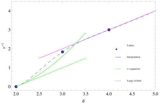
Figure 1.
Universal scaling exponent determining the running of G (see Equations (41), (70) and (62)) as a function of spacetime dimension d. Shown are the results in dimensions obtained from the exact solution of the lattice Wheeler–DeWitt equation [30,31], the numerical result in four dimensions [44], the expansion result to one [34] and two loops [35], and the large d result [53]. For actual numerical values, see Table 1.

Table 1.
Comparison of estimates for the universal gravitational scaling exponent , based on a variety of different analytical and numerical methods. These include the numerical results of [44], The expansion for pure gravity carried out to one and two loops [34,35], an estimate for the leading exponent in a truncated renormalization group expansion [54,55], a simple argument based on geometric features of the quantum vacuum polarization cloud for gravity [53], and finally the value obtained from consistency of the exact solution to the nonlocal field equation with a for the case of the static isotropic metric [56,57].
Another popular approach to the calculation of the universal exponent is based on a truncated renormalization group approach in the continuum in four dimensions. This gave values initially around [54,58] with some sizeable uncertainties; it is beyond the scope of this work to go into details regarding the features of each one of these calculations, so only a few representative cases are mentioned here. Recent improved functional renormalization group calculations tend to generally fall roughly in the region –. Studies using a bi-metric parameterization gave [59], and later in [60,61]. In [55,62], it was argued that only fluctuations should be included that have an on-shell meaning, in which case one finds , much closer to the lattice results. In [63,64], systematic studies were done of the dependence of the exponent on the metric parameterization and its influence on the functional measure contribution, giving generally for the leading exponents to lowest order. A similar value was found using a geometric flow in the linear approximation in [65]. Another systematic large parameter space investigation of gauge fixing and measure choices was done in [66], with estimates eventually falling within the above-mentioned range .
The graph in Figure 1 also includes the known exact result for quantum gravity in three spacetime dimensions, obtained from the exact solution of the Wheeler–DeWitt equation in dimensions, which gives exactly [29,30,31]. The latter universal exponent should be compared to the old numerical Euclidean lattice result in three dimensions [67], to the result of [35], and finally to the Einstein–Hilbert truncation results mentioned previously, which in three dimensions cluster around [68] and [65], again in general agreement with the trend found for the lattice results in the same number of dimensions.
Other lattice and continuum methods can be used to provide an estimate for the exponent in various spacetime dimensions. Results worth mentioning here include a simple argument based on the geometric features of the graviton vacuum polarization cloud, which gives for large d [53] (shown as a straight line in the graph of Figure 1), and the lowest order estimate for from the first nontrivial order in the strong coupling expansion of the gravitational Wilson loop [47], which gives . Finally, the results in [56,57] found that a consistent exact solution to the nonlocal effective field equations of Equation (72) (discussed below) for the static isotropic metric in can only be found provided exactly, in agreement with the geometric argument mentioned above.
4. Renormalization Group Running of Newton’s G
The results discussed thus far are helpful in establishing a direct connection between the fundamental gravitational correlation length and various diffeomorphism invariant averages such as the average local curvature and its fluctuation. In this framework, one can view the result of Equation (26) as equivalent to stating that the Callan–Symanzik renormalization group beta function has a non-trivial zero at . Generally, the cutoff independence of the nonperturbative mass scale in Equation (26) implies
Moreover, if one defines the dimensionless function via
then, from the usual definition of the Callan–Symanzik beta function , one obtains
It follows that the renormalization group -function, and thus the running of with scale, can be defined some distance away from the nontrivial fixed point; more generally, the running of is obtained by solving the differential equation
with obtained from Equation (36). Integrating Equation (37) close to the nontrivial fixed point, one obtains for
with an integration constant of the RG equations. It has dimensions of a mass or inverse length, so it is naturally identified with the invariant correlation length : . In particular, comparing results in Equations (26) and (38), one obtains
which implies that the universal exponent is directly related to the derivative of the Callan–Symanzik function in the vicinity of the fixed point at ; computing determines the universal running of G in the vicinity of . In addition, the renormalization group equations generally imply that the effective coupling will grow (anti-screening) or decrease (screening) with distance scale , depending on whether or , respectively. One crucial physical insight obtained from the lattice is that only the phase is physically acceptable [44]; the phase corresponds at large distances to an entirely unphysical, collapsed branched polymer with no sensible continuum limit.
From the previous discussion, one infers that the physical mass scale also determines the magnitude of the corrections to scaling, and plays therefore a role similar to the scaling violation parameter in QCD. As in gauge theories, this nonperturbative mass scale emerges dynamically even though the fundamental gauge boson remains strictly massless to all orders in perturbation theory, and consequently its mass does not violate any local gauge invariance. Furthermore, one expects, as in gauge theories, that in gravity the magnitude of cannot be determined perturbatively, and to pin down a specific value requires a fully nonperturbative approach, as given here by the lattice formulation. In turn, the genuinely nonperturbative physical mass parameter of Equation (26) is itself a renormalization group invariant and thus scale independent. In the immediate vicinity of the fixed point, it obeys the general renormalization group equation, which follows from Equation (34),
with an arbitrary momentum scale. Here again, by virtue of Equation (26), the second expression on the right-hand side is only appropriate in very close proximity of the fixed point at . Solving explicitly Equation (40) for , with q an arbitrary wave vector scale, one finally obtains for the running of Newton’s G with the action of Equation (2) or (5)
Here again, , and the coefficient for the amplitude of the quantum correction is , with from a numerical study of the decay of curvature correlation functions, and also as before [42,44]. Consequently, the dimensionless amplitude for the leading quantum correction in the lattice running of Equation (41) is . This then completely determines the running of G in the vicinity of the fixed point, namely for scales . Note that in the lattice theory of gravity only the smooth phase with exists (in the sense that an instability develops and spacetime collapses onto itself for ), which then implies that the gravitational coupling can only increase with distance (+ sign for the quantum correction in Equation (41)). In other words, a gravitational screening phase does not exist in the lattice theory of quantum gravity. The above situation appears to be true both for the Euclidean theory in four dimensions, and in the Lorentzian version in dimensions [30]. A better, covariant formulation for the running of Newton’s G is given later, in Equation (70). Note also that the domain of validity for the expressions in Equation (41) is or ; the strong infrared divergence at is largely an artifact of the current expansion, and should be regulated either by cutting off the momentum integrations at , or by the replacement on the r.h.s. .
It is clear that the magnitude of the quantum correction in Equation (41) depends crucially on the magnitude of the nonperturbative physical scale . It is argued below that this quantity is related, as in Yang–Mills theories, to the gravitational condensate, physically represented by the observed cosmological constant. Therefore, at this stage, it turns out that the only physically sensible interpretation is that the observed is tentatively related to the scale ,
From the above perspective, “short distances” are not really that short, since in comparison to G or the Planck length is a very large quantity, of cosmological magnitude. (The fundamental nonperturbative scale plays a crucial role in the following, and having a precise quantitative value for it is of paramount importance when trying to make contact with current astrophysical and cosmological observations. Here, for concreteness, a specific value in is assumed, in line with the most recent satellite data (see, for example, [69]). It is nevertheless quite possible that significant updates to this value will take place in the next few years, as increasingly sophisticated data, and data analysis methods, become available. One would nevertheless expect that various predictions, arising from the vacuum condensate framework described here, should lead to one single consistent value for the scale . In this context, it is worth remembering that before 1999 astrophysical observations were deemed to be entirely consistent with ). It follows that the reference scale for the running of G in Equation (41) is set by a correlation length which, by Equation (32) and after Equation (88), is related to the observed large-scale curvature. In particular, the specific form for the running of G with scale suggests that no detectable corrections to classical gravity should arise either (a) until the scale r approaches the very large (cosmological) scale or (b) until one reaches extremely short distances comparable to the Planck length (at which point higher derivative terms, light matter corrections, and string contributions come into play). In other words, the results of Equation (41) (or later in the covariant form of Equation (70)) would imply that classical gravity is largely recovered on atomic, laboratory, solar, and even galactic scales, or as long as the relevant distances satisfy .
5. Gravitational Wilson Loop and Curvature Condensate
In gauge theories, the Wilson loop is known to play a central role: on the one hand, it is a manifestly gauge invariant quantity, while, on the other hand, it provides key physical information on the nature of the static potential between two quarks. In gravity. it is possible to construct a close analog of the gauge Wilson loop, by taking the path-ordered product of rotation matrices (describing the parallel transport of a vector, and thus specified in terms of the affine connection) along a closed loop. Nevertheless, this path ordered product is not related to the gravitational potential; the latter is obtained from a different set of observables which involve the correlations of particle world lines modacorr, modaloop. Instead, the gravitational Wilson loop provides information, as already in the infinitesimal loop case, on the behavior of curvature on very large scales.
The required integration over rotation matrices (or, equivalently, the integration over the affine connection) is most easily done in a first order formulation, where the affine connection and the metric are considered as independent degrees of freedom. Such a formulation exists on the lattice [70] and is therefore most suitable for computing the gravitational Wilson loop [47]. As in the gauge theory case, the integration over rotation matrices is performed using an invariant Haar measure over the group, which then almost immediately leads to a (minimal) area law for the quantum gravitational Wilson loop,
Note that in the above expression use has been made of the fact that the basic reference scale appearing in the area law is the correlation length , a well-known scaling result in gauge theories and justified there by renormalization group arguments. In addition, C denotes the closed path that defines the loop; a more precise definition of the gravitational loop [47] is given further below. Suffice it to say here that the use of the Haar measure over rotations assumes and implies large local fluctuations in the metric, and thus in the affine connection, which is certainly justified for large G, where gravitational fluctuations in different spacetime regions decouple.
On the other hand, a macroscopic semiclassical observer is led to relate the parallel transport of a coordinate vector around a very large closed loop, via Stoke’s theorem, to the value of the locally measured curvature. This then leads immediately to the semiclassical result [47]
where R is a measure of the slowly varying local macroscopic curvature; again, a more precise definition is given further below. Comparing the quantum result of Equation (43) to the semiclassical result of Equation (44) (which is feasible since both contain the minimal area A of the loop in question) then provides a more or less direct relationship between the local large scale, semiclassical curvature R and the correlation length , namely , a result already alluded to above in Equation (42).
This last set of considerations in turn provides a further key ingredient in quantum gravity, namely the correspondence between the macroscopic semiclassical curvature and the invariant correlation length . One immediate consequence is that the scale for quantum effects in Equation (41) is related to the observed cosmological constant, which in quantum gravity acts effectively as an infrared regulator. Thus potentially serious infrared divergences associated with the masslessness of the graviton are regulated by this new nonperturbative scale , a mechanism that is similar to the way infrared divergences regulate themselves dynamically in QCD and non-Abelian lattice gauge theories. Consequently, the scale plays a role which seems analogous to the scaling violation parameter in QCD; one important difference is that the running of G, due to the existence of a nontrivial fixed point, is not logarithmic. Instead, the correct scale dependence of G is given by Equation (41) and thus follows a power law, with an exponent related to the derivative of the beta function at the fixed point in G.
A second crucial consequence is that the scale for quantum effects is not given by Newton’s constant; it is given instead by the size of , which because of its relationship to the cosmological constant is a very large, cosmological scale of the order of cm. It would seem therefore that such quantum effects will only become detectable when one explores the nature of gravity on cosmological scales comparable to . The running of G is exceedingly tiny on solar system and galactic scales, but nevertheless increases dramatically as one approaches distance scales which are comparable to the observed cosmological constant . What then remains to be done is therefore to incorporate the above running of G into a set of generally covariant equations which can then be applied to the calculation of quantum corrections to known classical gravity results at very large distances. This is discussed below. (Note that in gauge theories the correlation length can be determined directly numerically by investigating the decay of Euclidean correlation functions of suitable local operators as a function of the separation distance. Generally, these correlation functions are dominated by the lightest particle with a given spin. In the case of gravity, such a detailed and complete analysis has not been performed yet, although it is in principle feasible, just as it is in lattice QCD. One complication that arises in the case of gravity is the fact that correlation functions between invariant local operators have to be computed at a fixed geodesic distance [42]. The latter of course fluctuates, depending on the choice of background metric configuration used in evaluating the Feynman path integral.)
It is important at this stage to understand where the Wilson loop relationship in Equations (43) and (44) is coming from. A precise definition of the gravitational Wilson loop was given in [43,45,47]. First note that infinitesimal transport loops appear already, for example, in the definition of the correlation function for the scalar curvature, Equation (18). Here what is considered instead is the parallel transport of a vector around a loop C which is not infinitesimal. In the following, this loop is assumed to be close to planar, a well-defined geometric construction described in detail in [47]. First define the total rotation matrix along the path C via a path-ordered () exponential of the integral of the affine connection ,
The lattice action itself already contains contributions from infinitesimal loops, but more generally one might want to consider near-planar, but noninfinitesimal, lattice closed loops C. To make the above expression well defined, it needs to be put on a lattice. There one defines a finite product of elementary rotations defined along a given lattice path
The introduction of such rotation matrices in the Regge–Wheeler lattice is discussed in detail in [25,26,47], and a first order lattice formulation for gravity based on it is given in [70]; the following discussion is based this well understood formalism. A coordinate scalar can then be defined by contracting the above rotation matrix with a unit length area bivector , representative of the overall geometric features of the loop. Now, if the parallel transport loop in question is centered at the point x, then one can define the operator by
with the near-planar loop centered at x and of linear size . Of course, for an infinitesimal loop, involving an infinitesimal lattice path of linear size , the overall rotation matrix is given by
where now is the area bivector associated with the infinitesimal loop of area , and the corresponding deficit angle; here, R is lattice Riemann tensor at the hinge (triangle) in question, and the corresponding area bivector. Then, an invariant correlation function between two such operators is given by
with the two loops separated by some fixed geodesic distance d, as shown in Figure 2. Of course, for infinitesimal loops, one recovers the expressions given above in Equations (18) and (19).
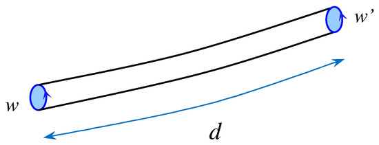
Figure 2.
Correlation function of two infinitesimal parallel transport loops, separated by a geodesic distance d. This correlation corresponds to the one defined in Equations (18) and (19). In the strong coupling limit, one needs, in order to get a non-zero correlation, to fully tile the minimal tube connecting the two infinitesimal initial and final loops.
In general, one needs to specify the relative orientation of the two loops. Thus, for example, one can take the first loop in a plane perpendicular to the direction associated with the geodesic connecting the two points, and the same for the second loop; the parallel transport of a vector along this geodesic will then be sufficient to establish the relative orientation of the two loops. Nevertheless, if one is interested in the analog (for large loops) of the scalar curvature, then it would be adequate to perform a weighted sum over all possible loop orientations at both ends. This is in fact precisely what is done for infinitesimal loops of size , if one looks carefully at the way the Regge lattice action was originally defined.
It is possible to give a more quantitative description for the behavior of the loop–loop correlation function given in Equation (49), at least in the strong coupling limit. Figure 3 shows the Correlation function for two large parallel transport loops of size and orientation , separated by a geodesic distance d. This correlation corresponds to the one defined in Equation (49). In the strong coupling limit, one needs, in order to get a non-zero correlation, to fully tile the tube connecting the two large initial and final loops. The following estimate is based on the previous results and definitions, and is further illuminated by the important analogy and correspondence of lattice gravity to lattice non-Abelian gauge theories outlined in detail in [47,53]. First, it is convenient to assume that the two (near planar) loops are of comparable shape and size, with overall linear sizes and perimeter . In addition, the two loops are separated by a distance , and for both loops it is assumed that this separation is much larger than the lattice spacing, and . Then, to get a nonvanishing correlation in the strong coupling, large G limit it will be necessary to completely tile a tube connecting the two loops, due to the geometric minimal area law arising from the use of the uniform (Haar) measure for the local rotation matrices at strong coupling, again as discussed in detail in [47]. Quite generally in this limit one expects an area law for the correlation between gravitational Wilson loops (see also the discussion for the Wilson loop itself given later below), which here takes the form
with the minimal area of the tube connecting the two loops. Consistency of the above expression with the corresponding result for small (infinitesimal) loops given in previously in Equation (22) requires that for small loops (small L) the value of L saturates to , , so that the correct exponential decay is recovered for small loops.
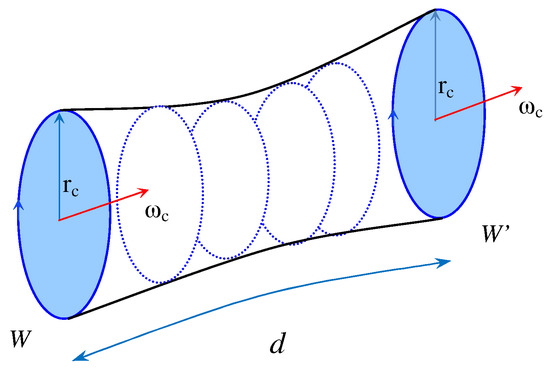
Figure 3.
Correlation function for two large parallel transport loops of size and orientation , separated by a geodesic distance d. This correlation corresponds to the one defined in Equation (49). In the strong coupling limit, one needs, in order to get a non-zero correlation, to fully tile the tube connecting the two large initial and final loops.
This result is not unexpected, since can only come into play only for distances much larger than the fundamental lattice spacing a. Consequently, the asymptotic decay of correlations for large loops is somewhat different in form as compared to the decay of correlations for infinitesimal loops, with an additional factor of appearing for large loops; nevertheless, in both cases, one has the expected minimal area law. In other words, the results of Equations (20) and (22) only apply to infinitesimal loops, which probe the parallel transport on infinitesimal (cutoff) scales; these results then need to be suitably amended when much larger loops, of semiclassical significance, are considered.
The above result applies to strong coupling, . As one approaches the critical point at more than one exponential will contribute, in analogy to Equation (20) for the single plaquette correlation. If the single loop contribution is proportional, as in the area law of Equation (50), to with , then for a spectral function one obtains, in the limit of a small infrared cutoff ,
Consistency of this expression with the infinitesimal loop result of Equation (20) then fixes and . For large loops, one obtains
Furthermore, from , as in Equation (20), one has , which gives for large (non-infinitesimal) loops of linear size L the following result, valid in the vicinity of the fixed point ,
This last function describes the correlation of large, macroscopic parallel transport loops of linear size , separated by an invariant distance d. Note the additional suppression, by a factor of when compared to the infinitesimal loop correlation function of Equations (20) and (24); for a macroscopic (semi-classical) parallel transport loop one has . Note that due to the dimensions of the curvature correlation function (see Equation (18)) the constantA has dimensions of one over length squared, with dimensionless. Furthermore, it is important to note that when the correlation of larger (i.e., non-infinitesimal) loops are considered the power law decay is unchanged, only the amplitude gets modified (compare Equation (53) with Equations (20) and (24) given above for infinitesimal loops; in both cases, the dependence on the separation is ). Again, to clarify, Equation (50) describes the exponential “large distance” () behavior of the loop correlation function, whereas Equation (53) describes the power law “short distance” () behavior of the same loop correlation function. Thus, the above result is analogous to what was found in Equation (22) describing there, on the one hand, the exponential “large distance” () behavior of the microscopic curvature (infinitesimal loop) correlation function, and on the other hand, from Equation (20), the power law “short distance” () behavior of the same correlation function.
One crucial ingredient needed in pinning down the magnitude of the quantum correction for in Equations (41) or (70), as well as the result for the loop correlation function of Equation (53), is the actual value of the genuinely nonperturbative reference scale . It is argued in [47] that, in analogy to ordinary gauge theories, the gravitational Wilson loop itself provides precisely such an insight. The main points of the argument are rather simple, and can thus be reproduced in just a few lines. In analogy to the gauge theory case, these arguments rely generally on the concept of universality, the existence of a universal correlation length at strong coupling, and the use of the Haar invariant measure to integrate over large fluctuations of the metric, or of the fundamental local parallel transport matrices. Following [45,46], in [47], the vacuum expectation value corresponding to the gravitational Wilson loop is naturally defined as
Here, the Us are elementary rotation matrices, whose form is determined by the affine connection, and which therefore describe the parallel transport of vectors around a loop C (see also Equation (46)). Again here, is a constant unit bivector, characteristic of the overall geometric orientation of the loop, giving the notion of a normal to the loop. In the continuum, the combined rotation matrix is given by the path-ordered () exponential of the integral of the affine connection , as in Equation (45), so that the previous expression represents a suitable discretized and regularized lattice form. It can then be shown [47] that quite generally in lattice gravity, and for sufficiently strong coupling, one obtains universally an area law for large near planar loops as advertised in Equation (43)
where is the geometric minimal area of the loop as spanned by a given perimeter. (In Wilson’s lattice formulation [20], this is a standard textbook result for non-Abelian gauge theories, see for example [71,72], specifically Equation (22.3) in the second reference. There represents the gauge field correlation length, or the inverse of the lowest glueball mass; here following [47] the gravitational result is written in the same invariant scaling form involving the fundamental nonperturbative correlation length .) This last result relies on a modified first order formalism for the Regge lattice theory [70], in which the lattice metric degrees of freedom are separated out into local Lorentz rotations and tetrads. Moreover, the result of Equation (54) is in fact rather universal, since it can be shown to hold in all known lattice formulations of quantum gravity at least in the strong coupling (large G) regime. In [47], an explicit expression for the correlation length appearing in Equation (55) was given in the strong coupling limit. There one finds . For k close to this then gives immediately and thus, to this order, in Equation (26). Nevertheless, the discussion of the previous sections and the numerical solution of the full lattice theory suggests that the correct expression for to be used in Equation (55) should be the one in Equation (26), with [Equation (28)], given in Equation (28) and amplitude .
One then needs to make contact between these results and a semiclassical description, which requires that one connects the nonperturbative result of Equation (55) to a suitable semiclassical physical observable. By the use of Stokes’s theorem, semiclassically the parallel transport of a vector round a very large loop depends on the exponential of a suitably coarse-grained Riemann tensor over the loop. In this semiclassical picture, one has for the combined rotation matrix
where is an area bivector, . The above semiclassical procedure then gives for the loop in question
Here, is a constant unit bivector, characteristic of the overall geometric orientation of the parallel transport loop. For a slowly varying semiclassical curvature, the R contribution can be taken out of the integral, so that the remaining integral depends on the overall large loop with some minimal area , for a given perimeter C. Then, by directly comparing coefficients for the two area terms in Equations (55) and (57), one concludes that the average large-scale curvature is of order , at least in the strong coupling limit [47]. Since the scaled cosmological constant can be viewed as a measure of the intrinsic curvature of the vacuum, the above argument then leads to an effective positive cosmological constant for this phase, corresponding to a manifold which behaves semiclassically as de Sitter () on very large scales [47]. For related interesting ideas, see also [73].
The above arguments then lead to the following key connection between the macroscopic (semiclassical) average curvature and the nonperturbative correlation length of Equations (22), (41), (62) and (70), namely
at least in the strong coupling (large G) limit. It is important to note that the result of Equation (58) applies to parallel transport loops whose linear size is much larger than the lattice spacing, ; nevertheless, in this limit, the answer for the macroscopic curvature in Equation (58) becomes independent of the loop size or its minimal area [47]. Furthermore, these arguments lead, via the classical field equations, to the identification of with the observed (scaled) cosmological constant (up to a constant of proportionality, expected to be of order unity)
In this picture, the latter is regarded as the quantum gravitational condensate, a measure of the vacuum energy, and thus of the intrinsic curvature of the vacuum [47]. It is nonzero as a result of nonperturbative graviton condensation.
The above considerations can finally contribute to providing a quantitative handle on the physical magnitude of the nonperturbative scale . From the observed value of the cosmological constant (see, for example, the 2015 Planck satellite data [69]) one obtains a first estimate for the absolute magnitude of the scale ,
Irrespective of the specific value of , this would indicate that generally the recovery of classical GR results happens for distance scales much smaller than the correlation length . (The value for , and therefore , relies on a multitude of current cosmological data, which nowadays is usually analyzed in the framework of the standard model. Included in the usual assumptions is the fact that Newton’s G does not run with scale. If such an assumption were to be relaxed, it would affect a number of cosmological parameters, including , whose value could then change significantly. In the following, the estimate of Equation (60) is used as a sensible starting point.) In particular, the Newtonian potential is expected to acquire a tiny quantum correction from the running of G (see Equation (70))
For example, in the case of the static isotropic metric, one finds that is given explicitly by [57]
with , so that quantum effects become negligible on distance scales . (The quantum gravity correction is reminiscent of the Uehling term in QED; nevertheless, the latter is purely logarithmic, and the infrared cutoff there is provided by the smallest mass scale appearing in QED loop corrections, the renormalized electron mass. In quantum gravity, the role of the infrared cutoff is played by the graviton mass, which in perturbation theory (as in Yang–Mills theories) stays strictly zero to all orders, due to local coordinate invariance).
One might think perhaps that the running of G envisioned here might lead to observable consequences on much shorter, galactic length scales. That this is not the case can be seen, for example, from the following argument. For a typical galaxy, one has an overall size ∼, giving for the quantum correction the estimate, from Equation (62) for the static potential, which is tiny due to the large size of (see Equation (60)). It seems therefore unlikely that such a correction will be detectable at these scales, or that it could account, in part, for anomalies in the galactic rotation curves. The above argument nevertheless shows a certain sensitivity of the results to the value of the scale ; thus an increase in by a factor of two tends to reduce the effects of by , as can be seen from Equation (70) with and the fact that the amplitude of the quantum correction is always proportional to the combination . Figure 4 shows the expected qualitative behavior for the running over scales slightly smaller or comparable to . The main uncertainty arises from estimating the physical magnitude of itself [see Equation (60)]. Specifically, from Equation (41) the lattice prediction at this point is for roughly a 5% effect on scales of , and a 10% effect on scales of .
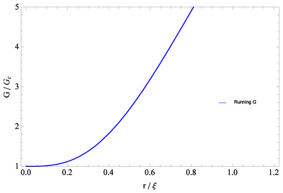
Figure 4.
Running gravitational coupling versus r, obtained from in Equation (41) by setting with an exponent . In view of Equation (42), lattice quantum gravity calculations imply a slow rise of G with distance scale, with roughly a 5% effect on scales of ≈790 Mpc, and a 10% effect on scales of ≈990 Mpc. In this plot, , the short distance fixed point value for Newton’s constant, corresponds quite closely to the known laboratory value.
Figure 5 shows how the lattice running of , given earlier in Equation (41), compares to the continuum analytical self-consistent Hartree–Fock solution to Dyson’s equations for quantum gravity, obtained recently in [74]:
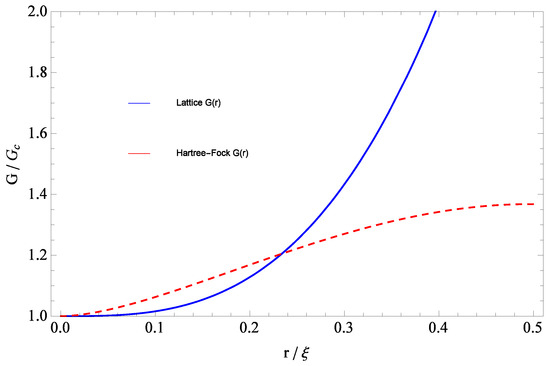
Figure 5.
Running gravitational coupling versus r, obtained from in Equation (41) by setting with an exponent . Note that the approximate Hartree–Fock analytical result of Equation (63) (red line) initially rises more rapidly for small r. The nonperturbative scale is related to the gravitational vacuum condensate, as in Equation (42).
Here again, m is related to the gravitational correlation length via (see Equations (59) and (60)). One notes therefore that the Hartree–Fock approximation to the self-consistent equation for the graviton vacuum polarization tensor also predicts an infrared rise of (antiscreening), and furthermore unambiguously determines the amplitude of the quantum correction (, here equal to ). In this approximation, the mean field result for the exponent is , so that the power is equal to two for Equation (63) in four dimensions. Thus, there are two main differences that stand out compared to the lattice result of Equation (41), namely that the power is two here and not three, and the fact that here there is an additional, slowly varying component (One of the earliest applications of the Hartree–Fock approximation to solving Dyson’s equations for propagators and vertex functions was in the context of the BCS theory for a superconductor. Later, it was applied to a (perturbatively non-renormalizable) relativistic theory of a self-coupled Fermion, where it provided the first convincing evidence for a dynamical breaking of chiral symmetry and the emergence of Nambu–Goldstone bosons [75]).
The above results also suggest that the curvature on very small scales behaves rather differently from the curvature on very large scales, due to the quantum fluctuations eventually averaging out. Indeed, when comparing the result of Equation (32) to the one in Equation (58), one is led to conclude that the following change has to take place when going from small (linear size ) to large (linear size ) parallel transport loops
An intuitive way of understanding the above result is that on small scales the strong local fluctuations in the metric/geometry lead to large values for the average rotation of a parallel-transported vector. However, on larger scales, these short distance fluctuations tend to average out, and the combined overall rotation is much smaller, by a factor of ,
The above quantity should then be regarded as an essential and necessary “renormalization constant” when comparing curvature on different length scales, and specifically when going from very small (size ) to large (size ) parallel transport loops. See also the earlier discussion preceding Equation (50), about the issue of comparing correlations of large loops versus correlations of small (infinitesimal) loops.
To conclude this section, one can raise the legitimate concern of how these results are changed by quantum fluctuations of various matter fields; thus far, all the results presented here apply to pure gravity without any matter fields. Therefore, here, and in the rest of the paper, what has been applied is basically the quenched approximation, wherein gravitational loop effects (perturbative and nonperturbative) are fully accounted for, but matter loop corrections are initially neglected. When adding matter fields coupled to gravity (scalars, fermions, vector bosons, spin-3/2 fields, etc.), one would expect, for example, the value for to change due to vacuum polarization loops containing these fields. A number of arguments can be given though for why these effects should not be too dramatic, unless the number of light matter fields is rather large [44]. (One would expect that significant changes to the result of Equations (41) and (70) will arise from matter fields which are light enough to compete with gravity, and whose Compton wavelength is therefore comparable to the scale of the gravitational vacuum condensate, or observed cosmological constant , namely . At present, the number of candidate fields that could fall into this category is rather limited, with the photon and a near-massless gravitino belonging to this category. The results presented here correspond to the quenched approximation for quantum gravity, where all graviton loop effects are included, but matter (and radiation) loops are neglected. Matter fields are still present in the theory but are treated as quantum mechanical static sources. In the perturbative expansion for quantum gravity, one encounters factors of in the renormalization groups function, where c is the central charge associated with the (massless) matter fields [34,35], which would suggest that matter loop and radiation corrections are indeed rather small. In four dimensions, similar factors involve [76,77], which would again lend support to the argument that such effects should be rather small in four dimensions.)
Note that the above results for the gravitational condensate in many ways parallel what is found in non-Abelian gauge theories, where for example one has for the color condensate [78,79,80,81]. In QCD, this last result is obtained from purely dimensional arguments, once the existence of a fundamental correlation length (which for QCD is given by the inverse mass of the lowest spin zero glueball) is established. Accordingly, for gravity, one would in fact expect simply on the basis of purely dimensional argument that the large scale curvature (corresponding to the graviton condensate) should be related to the fundamental correlation length by , as in Equation (32). This then points to a fundamental relationship between the nonperturbative scale (or inverse renormalized mass) and a nonvanishing vacuum condensate for both of these theories, nonperturbative quantum gravity and QCD,
In gauge theories, an additional physically relevant example is provided by the fermion condensate,
arising as a non-trivial consequence of the renormalization group, confinement and chiral symmetry breaking in SU(3) gauge theories [82]; for a recent review on current values (see, for example, [83]). Note that in all three cases the power of is fixed by the canonical dimension of the corresponding field, one over length square in the case of the curvature, an observation which can be seen to provide further support to the identification in Equations (58) and (59), which arise from considering the gravitational Wilson loop. The actual physical values for the QCD condensates are well known; current lattice and phenomenological estimates cluster around and [80,81]. On the other hand, modifications to the static potential in gauge theories are best expressed in terms of the running coupling constant , whose scale dependence is determined by the celebrated beta function of . There the relevant scale is the nonperturbative whose size is comparable to , . More specifically, in gauge theories, the inverse of the correlation length corresponds to the lowest mass excitation, the scalar glueball with mass . If the lightest scalar glueball has a mass of approximately (which then fixes at about ), then in QCD is about eight times smaller. Of course, one important difference between nonperturbative gravity and QCD is the fact that in the former the cutoff still appears explicitly, hidden in the physical value of Newton’s constant G (which is dimensionful). Thus, there exists then a second dynamically generated scale , whose magnitude is not directly related to the value of G; instead it reflects how close the bare G is to the fixed point value . Finally, it should be added that the idea of a graviton condensate as described here, and thus arising from non-perturbative gravity effects, is not entirely new. Interesting papers looking into such effects—but based on entirely different assumptions and therefore from a rather different perspective—can be found for example in [84,85].
6. Effective Field Equations
The result of Equation (41) expresses the renormalization group running of Newton’s G as a function of momentum scale. As it stands, the expression in Equation (41) does not satisfy general covariance, and needs to be promoted to a more useful and acceptable form. It follows that, to apply consistently the above result to an arbitrary background geometry, a fully covariant formulation is required. One way of describing the running of Newton’s G is by a set of effective nonlocal field equations with a [41,56]. A second option is to formulate a fully covariant effective gravitational action with a running , also discussed in detail in [41,56]. In the following, both options are discussed. This general approach, originally pioneered by Vilkovisky [86], has had great success in incorporating in a gauge independent way the renormalization group running of the coupling in gauge theories such as QED and QCD. (A precursor to the effective action approach involving the running of G can be found to some extent in the Brans–Dicke scalar-tensor modification of Einstein’s gravity [75], where Newton’s constant is promoted to a field-dependent quantity, as a result of incorporating in a partial way the requirements of Mach’s principle regarding the origin of inertia. Nevertheless, the two approaches remain quite different, in the sense that the discussion here is strictly limited to what is expected on the basis of a quantum field theoretic treatment of Einstein’s gravity with a cosmological constant, and suitable additional known matter fields. A Brans–Dicke type of extension of the current quantum theory is possible, say by the addition of a dynamical massless scalar field with suitable covariant couplings, but are not considered here).
An effective field theory approach can be derived by writing down an effective action, involving either a or a [41,56]. Based on the previous discussion, a suitable effective action, describing the residual effects of quantum gravity on very large distance scales, is of the form
with a very slowly varying (on macroscopic scales) Newton’s constant, in accordance with Equations (41) or (70), and amplitude [44]. Note that the effective action of Equation (68) is obtained from the one in Equation (2) by a suitable field rescaling, in accordance with the discussion preceding Equation (9). Here again, the nonperturbative scale appears therefore both in the running of G and in the cosmological constant term with . Nevertheless, it was found that if a covariant is used in the above effective action the resulting effective field equations are rather complicated and hard to solve in practice, due to the fractional exponents appearing in [41,56].
For reasons that become clearer below, in most of the upcoming discussion, a different route is followed, based on the much simpler (and thus more manageable) effective field equations based nevertheless again on . In either case, it seems natural to perform the standard quantum mechanical replacement , where is the covariant D’Alembertian for a given background metric [56],
This then leads to a consistent covariantly formulated running of G, with
Note that the precise form of the covariant □, and thus of , depends on the tensor nature of the object it acts on [56]. Numerical studies of lattice quantum gravity give for the exponent and for the quantum amplitude [44], which (fortunately or unfortunately) leaves very little ambiguity regarding the result of Equation (70). As noted above, one way of viewing physically the result of Equation (70) is that quantum gravitational fluctuations generate anti-screening, with an initially very slow running of G, as shown earlier in Figure 4. The anti-screening arises because of the radiative dressing of the source by a virtual gravitation graviton cloud, in analogy to the screening of a bare charge in QED by the virtual electron-positron cloud. In a sense, therefore, the above corrections describe the gravitational analog of the running coupling constant in QED.
Generally, fractional powers of inverse d’Alembertians require careful handling. This can be done either by computing the effect of integer powers and then analytically continue the result to fractional negative values , or by using a regulated parametric integral representation
where is a suitable infrared regulator, here again with exponent . Note that for the quantum correction in Equation (70) proportional to always includes a , which therefore naturally sets the overall scale for the leading quantum correction, irrespective of the background geometry considered. Then, a suitable set of manifestly covariant effective field equations with a running takes the form [56]
with the additional nonlocal contribution coming from the quantum correction in the of Equation (70). It is important to note that the nonperturbative scale enters the effective field equations in two places, first in the cosmological constant term of Equation (42) due to the non-vanishing vacuum condensate discussed above, and also in the running of G of Equation (70) where it sets the reference scale. A clear implication here is that those two scales, which in principle could be entirely unrelated, appear to be one and the same in the present renormalization group context. The nonlocal, but manifestly covariant, effective field equations of Equation (72) can then, at least in principle, be solved for a number of physically relevant metrics. For the specific case of a static isotropic metric, it is possible to obtain an exact expression for in the limit [56], a result given previously in Equation (62). Not unexpectedly, generally all three expressions in Equations (41), (62) and (70) are consistent with a gradual slow increase in G with distance r, and thus with a modified Newtonian potential in the same limit (It is useful to observe here, quite generally and independent of the lattice results, that one finds it difficult to implement a weakly running cosmological constant, if general covariance is to be maintained at the level of the effective field equations. If the running of is implemented via a , then because of one also has , which makes it nearly impossible to maintain general covariance and have a nontrivial running , as pointed out in [41]).
Naturally, the next step is a systematic examination of the nature of solutions to the full effective field equations of Equation (72), with involving the covariant d’Alembertian of Equation (69), acting there on the second rank tensor . A scale-dependent Newton’s constant is then expected to lead to small modifications of the standard cosmological solutions to the Einstein field equations, proportional to the amplitude . Already, the action of is rather complicated on second rank tensors; one has
and
Of course, one of the simplest applications is to the Friedmann–Lemaître–Robertson–Walker (FLRW) framework applied to the standard homogeneous isotropic metric
in the following only the case (spatially flat universe) is discussed. In this framework, a popular choice for is the perfect fluid form,
for which one needs to compute the action of on , and then analytically continues the answer to negative fractional values of . The results of [56,57,87] then show, among other things, that a nonvanishing pressure contribution is generated in the effective field equations, even if one initially assumes a pressureless fluid, . Specifically, for a universe filled with nonrelativistic matter (p = 0), one obtains the following set of effective Friedmann equations,
for the field equation, and
for the field equation. In the above expressions, the running of G appropriate for the Robertson–Walker metric is
with (for an amplitude appearing in Equation (70)) for the tensor box operator [56]. From the above form of , one sees that again the amplitude of the quantum correction is proportional to the combination for . Furthermore, the running of G induces an effective pressure term in the second () equation, due to the presence of an induced relativistic fluid, whose origin lies in the quantum gravitational vacuum-polarization contribution. Another noteworthy feature of the new effective field equations is the additional power-law acceleration contribution, on top of the standard exponential one due to the term.
On way of viewing the results is that the effective field equations with a running G, here Equations (76) and (77), can be recast in an equivalent form by defining a vacuum-polarization pressure and density , such that in the FLRW background one has
From this viewpoint, the inclusion of a vacuum-polarization contribution in the FLRW framework amounts to a replacement , in the original field equations. Then, just as one introduces a parameter w, describing the matter equation of state,
with for nonrelativistic matter, one can do the same here for the remaining quantum contribution by setting
The original calculations in [56], and more recently in [88] (which includes metric perturbations), give . Note that it is shown in [56] that this result is obtained generally for the given class of considered, and is not tied to a specific choice for the universal exponent , such as .
More generally, the procedure of defining a and a contribution, arising from quantum gravitational vacuum-polarization effects, is not necessarily restricted to the FLRW background metric case. One can always decompose the full source term in the effective nonlocal field equations of Equations (70) and (72), making use of
as two contributions,
The latter then involves the nonlocal part
Consistency of the full nonlocal field equations now requires that the sum be covariantly conserved,
In general, one cannot expect that the contribution will always be expressible in the perfect fluid form of Equation (75), even if the original for matter (or radiation) has such a form. The former will in general contain, for example, nonvanishing shear stress contributions, even if they were originally absent in the matter part [88]. Indeed, in a number of cases of physical interest, one deals quite generally with a background metric that is slightly perturbed, . Consequently, the covariant d’Alembertian operator acting on second rank tensors (such as the in Equation (72)) needs to be Taylor expanded in the small perturbation h,
For itself, one obtains the expansion
to which one can apply the binomial formula . This then allows one to work out in some detail a number of predictions that arise from the original manifestly covariant effective field equations, Equation (72). It is also customary to later expand the relevant fields (metric perturbations, matter perturbations, etc.) in Fourier modes, with the small k modes as the leading contribution, and higher modes treated later again as perturbations. This nevertheless significantly complicates further the analysis of the results [88,89], given the intrinsic dependence on scale k of the quantum correction in G, see for example Equation (41) for or its equivalent covariant form of in Equation (70).
7. Large Scale Curvature and Matter Density Correlations
Quantum gravity, and the existence of a nontrivial quantum condensate for the curvature, lead to a number of specific physical predictions, which are in principle observationally testable. Many of these quantum correction effects can in principle be calculated, given the effective long-distance quantum corrected gravity theory formulated in Equations (70) and (72). The most salient effects include a running of Newton’s constant G with scale on very large (cosmological) scales; the modification of classical results for (relativistic) matter density perturbations and the associated growth exponents; a non-vanishing so-called slip function in the conformal Newtonian gauge; quantum effects that lead to nontrivial curvature, and therefore matter density, correlations at large distances, with the latter parameterized by a set of exponents characterizing the decay of correlation functions and their amplitudes, all of which are in principle calculable. As in the case of QCD and Yang–Mills theories, one expects essentially no adjustable parameters. Summarizing what has been stated before, one has that the running of G in Equation (72) is completely determined by the universal exponent , the nonperturbative quantum amplitude and the correlation length , which in turn is related to either the vacuum expectation value of the curvature, or to what is equivalent to it, the observed non-vanishing large-scale cosmological constant .
Much of what has been discussed so far was relates to the fact that in a quantum theory of gravity the gravitational constant G runs with scale, in accordance with Equation (70). However, there are additional consequences, which arise from the fact that in general gravitational correlations do not follow free field (Gaussian) predictions and which are therefore the subject of this section. One would expect such correlations to have some observational relevance, and one such example is the curvature correlation function of Equations (18) and (20), with power . However, it is useful to first examine some local averages. For the average local curvature , one has from Equation (32), using Equation (26) and ,
as given above in Equation (32). Lattice calculations allow one to extract various amplitude coefficients, such as the one in the above expression. The dimensionless amplitude in Equation (88) is expected to be in lattice units, and numerically one finds [44] . On the other hand, for the curvature fluctuation one has from Equations (13) and (33)
also given above in Equation (33). Note that, in both Equations (88) and (89), the correct dimensions have been restored, by inserting suitable powers of the lattice spacing a (curvature has dimensions of one over length squared); in addition, a specific value for this lattice spacing is given above in Equation (30). For the dimensionless amplitude in Equation (89), one finds numerically [44], again in general agreement with the prejudice that nonvanishing dimensionless critical amplitudes should be .
These results in turn provide some useful information related to the local curvature correlation function at a fixed geodesic distance (see Equations (18) and (19)). By scaling, one obtains immediately (from ) for the power appearing in Equation (20),
(One can contrast this result with what one finds in weak field perturbation theory. There one finds [45] and thus , so the result here is quite different. If one defines in the usual way an anomalous dimension for the graviton propagator in momentum space, , one finds from the lattice calculation or in four dimensions for , which deviates rather significantly from the Gaussian or perturbative value. Such a large deviation is already observed in the expansion (see Equation (39)) and is not peculiar to lattice quantum gravity; in the context of gravity such an interesting possibility was already discussed some time ago in [90].)
For the local curvature–curvature correlation function of Equation (18) at “short distances” (and again for ), one then obtains the rather simple result
As before, in the last term, the correct dimensions have been restored by inserting suitable powers of the lattice spacing a. The dimensionless amplitude of Equation (91) is related to the amplitude in Equation (89) because of Equation (25), and one finds from the numerical solution [44] , so that the dimensionless curvature correlation function normalization constant is . Again, as expected, this amplitude is close to in units of the cutoff (fundamental lattice spacing) a. Note that the two-point function result of Equation (93), and related to it the scaling dimension of Equation (90), also determines the form of the reduced three-point curvature correlation function
with a constant, and relative geodesic distances , etc. The relevance and measurement of nontrivial three- and four-point matter density correlation functions in cosmology was discussed in detail some time ago in [91].
It is instructive at this stage to compare the above result for the local curvature correlation given in Equation (91) to the expression for the local average curvature of Equation (88): both expressions still contain explicitly the size of the microscopic, infinitesimal parallel transport loop , which originates in the fact that both these quantities make explicit reference to infinitesimal (ultraviolet cutoff sized) parallel transport loops. The explicit appearance of the ultraviolet cutoff in these averages can be explained by the appearance of residual short distance divergences associated with such small infinitesimal loops. At the same time, a comparison of the result of Equation (88) for the local curvature with the corresponding result of Equation (58) for the large scale, macroscopic curvature suggests a substantial changeover when going from small (size ) to large (size ) parallel transport loops. As discussed above, the results can be summarized by the statement that the curvature on large (macroscopic) scales is much smaller (by a factor ) than the curvature on small (Planck length) scales, due to a dramatic averaging out of the fluctuations.
As described above in Equations (64) and (65), one then expects that the transition from infinitesimal to macroscopic loops (linear size ) can be affected in the correlation function of Equation (91) by the replacement of . This then would give for large (macroscopic size ) parallel transport loops a modified form of the correlation function of Equation (91)
with the general expectation that the overall amplitudes nevertheless be comparable, . Note that the universal power is unchanged compared to Equation (91), only the amplitude has been modified, in accordance with the above gravitational Wilson loop result of Equations (52) and (53). Unfortunately, thus far, these large loop correlations have not been computed explicitly, but nevertheless the above ideas should become testable by explicit numerical simulations in the near future.
The next step is to determine whether the knowledge of the curvature correlation, as given in Equations (91) or (93), can be translated into information regarding other two-point correlations subject to astrophysical measurement. First, consider what can be stated purely at the classical level. There one can use the field equations to directly relate the local curvature to the local matter mass density. From Einstein’s field equations with ,
for a perfect fluid one then obtains for the Ricci scalar, in the limit of negligible pressure,
This last result then relates the local fluctuations in the scalar curvature to local fluctuations in the matter density , and could therefore provide a potentially useful connection to the quantum result of Equations (20), (91) and (93). Note that the same kind of reasoning would apply alternatively to a describing radiation, which would then be relevant for a radiation-dominated early universe. Of course, in the Newtonian limit, the above result simplifies to Poisson’s equation
where and are the macroscopic gravitational field and the macroscopic mass density, respectively.
Now, in the current cosmology literature [91,92], it is customary to describe matter density fluctuations in terms of the matter density contrast correlation function (In cosmology the (dimensionless) galaxy matter density two-point function is usually referred to as , but here it seems desirable to avoid confusion with the gravitational correlation length )
The latter is related to its Fourier transform by
It has to contain, in general, both an infrared regulator () and an ultraviolet cutoff (), to make sure the integral stays convergent. If one assumes, as is sometimes the case, that the power spectrum is described by a simple power law
(where is commonly referred to as the spectral index), then one finds in the scaling regime for the real-space density contrast correlation function
provided the index s satisfies , and here (terms containing the ultraviolet cutoff appear as well, but they are proportional to and , oscillate rapidly and average out to zero). This then leads to the identification of exponents (see Equations (90) and (91)) or
For the specific value , one has , and therefore in position space
which is in fact, as discussed below, also consistent with the result given above in Equation (91) for the invariant, connected curvature correlation function.
Generally, all of the above expressions get modified for very small wave vector , as should be clear by now from the discussion in the previous sections, where the appearance of a dynamically generated infrared cutoff (as in QCD, and more generally in non-Abelian gauge theories) stood out as an essential ingredient. Such an infrared cutoff is either introduced explicitly in the wave vector integrations, or, alternatively, the power spectrum is infrared regulated at small q by replacing . (In perturbative QCD, the replacement partially accounts for the existence of (nonperturbative) infrared renormalon effects. In practice including these effects turns out to be, not surprisingly, phenomenologically quite successful, see for example [93,94] and references therein.) One then writes more appropriately, instead of Equation (99),
Again, by Fourier transforms, one then obtains for the correlation in real space
which reproduces Equation (100) for short distances . For very large spatial separations , the asymptotic behavior of is now given instead by
with amplitude . In view of the previous discussion, it is natural to identify here the infrared cutoff , and such a choice is implicit from now on throughout the following discussion. Note the correspondence of the result of Equation (100) with the short distance curvature correlation result of Equation (20), as well as the same type of correspondence of Equation (105) with the large distance curvature correlation result of Equation (22).
In practice, observational data for such matter density correlations is commonly presented in the following compact form [91]
with an empirically determined exponent , and a scale fitted to astrophysical (usually galactic cluster) observations. For close to two, one has by comparing Equation (102) to Equation (106) . It seems therefore rather tempting at this stage to try to connect the observational result of Equation (106) to the quantum correlation function in Equation (91). One then expects for the matter density fluctuation correlation a power law decay as well, of the form (ote that, in weak field perturbation theory, one finds, by virtue of the equations of motion, , so again the result here is rather different)
where here stands for the cosmological scale factor (The scale-factor dependent prefactor involving and has such a simple form only in a matter-dominated universe; for the a-dependent prefactor is a bit more complicated, nevertheless it still reduces to unity for equal times [92]). The last correlation function can be made dimensionless by suitably dividing it by the square of some average matter density with and for (using again, for concreteness, the Planck 2015 data [69]). By comparing powers and coefficients in Equations (91) and (106), one finds
For the reference scale in this last equation, one derives the quantitative estimate
with the dimensionless amplitude for the curvature correlation function of Equation (91), and a the lattice spacing given in Equation (30).
The preceding arguments, however, still contain a fundamental flaw, related to the use, at this stage in unmodified form, of the curvature correlation function result of Equation (91). As discussed above, that form applies to the correlation of infinitesimal (Planck length, or cutoff size) loops, which would not seem to be appropriate for the macroscopic (or semiclassical) parallel transport loops, such as the ones that enter the field Equations (94) and (95), and which thus relate locally the macroscopic to the . It would therefore seem desirable to be able to correct for the fact that the parallel transport loops sampled in Equation (95) are much larger than the infinitesimal ones sampled in the correlation function in Equation (91). As in Equations (64) and (65), the transition to macroscopic loops (linear size ) can be affected in Equation (91) by the replacement of . This then gives for large (macroscopic size ) parallel transport loops (see Equation (93))
with the expectation of a comparable amplitude . This last result then leads to the following improved estimate for the macroscopic matter density correlation of Equation (97),
so that comparing to Equation (106) one finds again for the exponent , and for the length scale the improved value
which now seems more in line with observational data. For the Fourier amplitude in Equation (99), one obtains the estimate
Observed galaxy density correlations give indeed for the exponent in Equation (106) a value close to two, namely for distances in the to range [91,95], and for the length scale , which is about two orders of magnitude smaller than the result of Equation (112) (using , see Equation (60)). More recent estimates for the exponent , going up to distance scales of , range between and [96,97,98,99,100,101]. The conclusions are similar if one looks at the galaxy power spectrum data, which also suggest assuming an exponent exactly, again consistent in view of Equation (113) with , a value that seems rather low (again by two orders of magnitude) in view of the original identification of as the vacuum condensate scale, Equations (58) and (60). Nevertheless, at this point, the (perhaps admittedly rather naive) identification given in Equations (112) and (113), while intriguing, is possibly entirely accidental. It largely bypasses any considerations regarding the actual physical origin (beyond the simple arguments given here) of the galaxy correlation function in Equation (109), including the model-dependent form and evolution of primordial density perturbations, the detailed nature of linear and non-linear relativistic matter density perturbation theory for a given comoving background etc.
Let us note here that the previous discussion focuses on the relationship between the curvature correlation and the matter density correlation, in accordance with Equations (20), (91) and the field equation result Equation (95). Nevertheless, for sufficiently small q, it is no longer legitimate to assume that Newton’s constant G is constant, as was done in Equation (95), and which later affects the results of Equations (109) and (113) to the extent that they involve G. Instead, one should make use of the effective field equations of Equation (72), which involve a running , or more simply make use of as given in Equation (41). When the above replacement is performed, one finds
with as before and (in view of the preceding discussion) still . Then, the most important modification, as can be seen quite clearly in Figure 6, is the rather dramatic decrease in magnitude (due to the factor) of for small , with a clear turnover at .
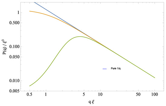
Figure 6.
Qualitative behavior of the (gravitational quantum fluctuation-induced) matter density power spectrum with a running Newton’s , as given explicitly in Equation (114). Here, it is compared to the results of Equations (99) and (103) for a constant G. In addition, the spectral exponent is and the amplitude is , as discussed in the text (see Equations (101) and (113)); in the plot, the q wave vector is measured for convenience in units of . Note the rather marked turnover for small due to the running of G, as discussed in the text. The nonperturbative scale is related to the gravitational vacuum condensate, as in Equations (59) and (58).
In view of the more complex behavior of , it is clearly no longer possible to associate a single spectral index with . Following Equation (99), one can nevertheless define an effective spectral index via
This quantity tends to for but then dips below zero for . A plot of is shown in Figure 7. One would expect that such a drastic turnover, caused by the quantum running of on very large scales, should become visible in future cosmological observations. From a practical perspective, it might make more sense to treat the numerical amplitude in Equation (93) as a free parameter, given the uncertainties, discussed above, associated in its determination from a first principle lattice calculation (see the discussion following Equation (110)). In other words, it would seem that so far, based on existing results, the q-dependence of is more credible at this stage than its overall normalization. A much more detailed and recent discussion of the expected behavior of the matter power spectrum and its extrapolation to the CMB regime, based on the vacuum condensate picture of quantum gravity presented here, can be found in the recent paper [102].
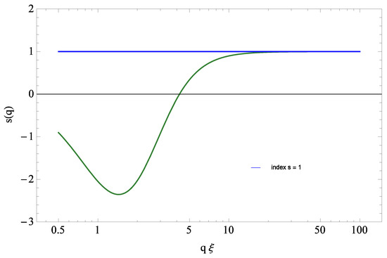
In conclusion, the main results of this section can be summed up as follows. The vacuum condensate picture of quantum gravity leads to three main predictions for matter density correlations, of which the first one is that the power appearing in Equation (106) should be exactly for “short distances” (or ), and that the reference length scale appearing in the same equation should be related to , as in Equation (112). The second prediction is that the power spectrum exponent in Equation (99) should be exactly again for , and that the amplitude in the same equation should be related to as in Equation (113). The third prediction is that the power spectrum as a function of q should exhibit a marked break for , as given later in Equations (103) and (114), and shown in Figure 5 and Figure 6 (A further complication arises in the cosmological context from the fact that at late times so that and are quite comparable in magnitude (which follows from the FRW evolution of the scale factor for a universe dominated by a term), whereas at early times a new, much shorter scale appears . Such effects are expected to play a role as well, and have not been taken into account here yet). More generally, the results outlined here and in the previous sections suggest that existing, and future, astrophysical and cosmological data should be re-analyzed in terms of a wider scale dependent form, similar to the one in Equation (41), and of the general (but rather simple) two-parameter type , with a wave vector reference scale, and p a positive power.
8. Gravitational Slip Function with
A running of Newton’s G gives rise to significant long-distance effects, which fundamentally modify the classical field equations of general relativity at very large distance scales. The following section provides an update on the results originally presented in [89], especially in view of the recent high accuracy lattice results presented in [44], and in particular related to the new improved estimate for the quantum amplitude of Equation (70). It is common practice to describe relativistic effects in cosmology within the framework of the comoving gauge, where the metric is written as
with background metric , fluctuations such that , with the remaining ’s decomposed into a trace and stress part
so that . In this gauge, the metric is then parameterized by the scale factor and the two additional functions s and h.
There are nevertheless instances where effects which deviate from standard Newtonian physics are more easily described within the context of the conformal Newtonian gauge, where the metric is parameterized by two scalar potentials and [103,104]. It is of some interest to explore possible cosmological consequences of a running Newton’s constant in this gauge, as discussed recently in [88]. In this gauge, one sets for the metric with , , and furthermore
with the components of again considered here as a small perturbation. The line element is then given by
Then, gravitational slip function is defined as
In classical General Relativity, one has giving then , which makes the quantity a rather useful parameterization for deviations from the classical theory (whatever their origin might be).
Generally, quantum corrections arising from a running of give rise to additional terms in the field equations, which no longer ensure that . In practice, at some stage of the calculation, one needs to compute higher order contributions from the ’s which requires one to expand, for example, in the metric perturbations , Consequently, the covariant d’Alembertian has to be Taylor expanded in the small field perturbation ,
and similarly for as in Equation (87), which requires the use of the binomial expansion for the operator . One has therefore
where the superscripts and refer to zeroth and first order in this weak field expansion, respectively. It is also customary in these treatments to expand all relevant fields in spatial Fourier modes. One sets for the matter density, pressure and velocity, as well as for the metric,
with the comoving wave number, and similarly for any of the other fields as well. An additional approximation is then to limit at first the treatment to the leading mode, and leave the more challenging corrections for a later calculation. Nevertheless, here the nonlocal nature of the quantum corrections makes the calculation of the slip function , as well as other quantities, technically rather difficult due to the intrinsic non-locality of in Equation (70), which will require at some stage a number of physically motivated approximations, so that a partial, useful answer can be obtained. Furthermore, the general result for the slip function is most easily presented in a form where the metric perturbation is decomposed into the comoving trace (h) and a stress (s) part; then, in the original comoving gauge, the spatial metric perturbation is written as in Equation (117). It is useful here to record the (rather straightforward) relationship between perturbations in the standard comoving and conformal Newtonian gauge, namely
Further details regarding the various choices of gauge (comoving, synchronous and conformal Newtonian) and their mutual relationship, as they apply to this specific problem, can be found in [89].
The zeroth order (in the metric perturbation ) the Friedman equations in the presence of a running G are given in the comoving gauge by
with for non-relativistic matter and for the graviton vacuum polarization contribution, together with the energy conservation equation
These equations need to be solved first to obtain an expression for the background scale factor as well as for the background average matter density . Of course, for , the above equations reduce to the standard Friedman equations with cosmological constant .
When restricted to the mode (the zeroth order, dominant infrared mode) one obtains for the slip function an expression which is a function of or , where t is the cosmological time and the corresponding scale factor. The detailed dependence of G on t or (and other parameters) is in turn quite sensitive to the specific choice of cosmological parameters, such as the rate of expansion, the relative contribution of dark matter versus dark energy, etc. In the end, one finds the following result for the slip function [89]
with given in Equation (78) and .
A specific numerical value for depends on various assumptions introduced in order to concretely evaluate the above expression. One of the simplest cases corresponds to the limit of a vanishing cosmological constant, . In view of Equation (59), this last limit corresponds to a very large . For a general perfect fluid with equation of state , one then has for the scale factor and for average matter density . Then, from Equation (127) one obtains for pure non-relativistic matter, ,
and more generally for
In both cases, the amplitude for the tensor box operator [56], with entering the expression for of Equation (70), and , giving therefore an overall coefficient . Another extreme, but equally simple, case is a pure cosmological constant term, which can be modeled by taking the limit .
To analyze the more general case of a non-vanishing cosmological constant combined with non-relativistic matter (), the following form [88] for the slip function expressed in terms of the scale factor turns out to be more useful
The integration constant is fixed by the requirement that the scale factor for (see Equations (70), (78) and (141) below for the definitions of ). In other words, by switching to the variable instead of t, the quantity has been traded for . In practice, the quantity is generally expected to be slightly larger than the scale factor “today”, i.e., for . As a result, the correction in Equation (130) is expected to be negative today. What is then needed is the general relationship between t and (for nonvanishing cosmological constant ) so that a quantitative estimate for the slip function can be obtained from Equation (130). Specifically, one is interested in the value of for a current matter fraction , as suggested by current astrophysical measurements (according to the recent Planck 2015 data, see [69]). To obtain , one then makes use of from Equation (78), and then substitutes the correct (matter-fraction dependent) relationship between t and a [89], which among other things contains the constant
with the parameter defined as
with the current () matter density, and the current matter fraction. In practice, one is interested in a matter fraction of around , giving , which is quite a bit larger than the zero cosmological constant value of . This then gives roughly and in Equation (130).
The last step left is to make contact with observationally accessible quantities, by expanding in the redshift z related to the scale factor by . For exponent and matter fraction one obtains for the gravitational slip function “today” ()
with . Here, f is a numerical constant equal to for pure non-relativistic matter ( and ), and for the current observed matter fraction (thus, but still ). Note that the correction is always negative, and since the above [see the mode expansion in Equation (123)] correction seems rather large in magnitude, . Nevertheless, one should keep in mind that the above result only corresponds to the extreme limiting case of comoving wavevector . In analogy to the quantum mechanical particle (the graviton) in a box, the lowest possible mode corresponds to where L is the linear size of the box. Here, the role of the L is played by the correlation length , so that the lowest possible mode corresponds in fact to , for which then the result of Equation (133) applies.
Generally, the quantum contributions to the slip function are scale dependent, and thus are proportionately reduced if one looks at scales that are significantly smaller compared to the largest scale in the problem, namely . The calculation of the slip function over a wider range of scales is clearly a significantly more complicated problem, which has not been addressed yet; as stated previously all calculations performed so far [89] only correspond to limit of , for which the above analytical estimate has been obtained. Nevertheless, if the corresponding relevant astrophysical length scale is denoted by , then at such a scale one must have, simply by scaling from Equations (41) and (70),
with given above in Equation (133). In other words, the result for is reduced by the ratio of the relevant length scale compared to or , to the third power since the exponent . As a practical example, if one were to look at the value of the slip function on scales which are an order of magnitude less than the reference scale , then this would reduce, in accordance with Equations (41) and (70) (where the correction is always proportional to ), the answer by a factor of . Thus, for distance scales (using again for reference ), one obtains from Equation (134) . For even shorter distance scales , one has , which is now a rather small number.
In practice, “large scales” in observational cosmology correspond to , with redshift surveys going up to scales of ∼, and recent CMB surveys probing scales up to ∼ (with current estimates of the scaled Hubble constant giving ). As far as astrophysical observations are concerned, current estimates for obtained from CMB measurements give values around [105,106], which could be used in the future to place a direct observational bound on the slip function of Equations (133) and (134).
9. Matter Density Perturbations with
The classical treatment of cosmological models in General Relativity usually starts out from a given background metric (such as the Friedmann–Lemaître–Robertson–Walker one), and then later uses the field equations to constrain small fluctuations about that metric. One application of this method is the computation of the gravitational growth of matter density perturbations , usually restricted in a first approximation to the lowest comoving spatial momentum modes. In this limit, the growth parameter obeys, as a function of scale , a rather simple ordinary differential equation, whose solution then provides, given suitable initial conditions, information about the matter and dark energy content of the current universe. One quantity that is often brought into play is the growth index , namely the derivative of the log of with respect to the log of the scale factor , and in addition the parameter , which provides information on how the growth index depends on the current matter fraction [91]. Cosmological observation suggests that today’s matter fraction is about [69], leading to a value of , based pretty much entirely on what is obtained from the systematic treatment of density perturbations within the framework of classical General Relativity.
It follows that many of the calculations just described can be repeated if one assumes now that Newton’s constant runs with scale, so that the standard field equations of GR get modified by the non-local term of Equation (70). Under the physically motivated assumption of a comparatively slowly varying (both in space and time) background, it is then possible to obtain a complete and consistent set of effective field equations, describing small perturbations for the metric trace and matter modes [88,89]. This then gives rise, within the same set of methods and approximations used in classical GR, to a set of equations for the growth amplitude. The latter are then studied again, initially, in the limit of small q wave vectors, and this in turn leads to modified growth exponents. In general, the results are expected to be quite sensitive to the scale , but so far only the leading term as goes to zero has been calculated analytically, due to technical difficulties which arise from the strong non-locality of . The following section provides a significant update on the results presented originally in [89], especially in view of the recent high accuracy lattice results presented in [44], and in particular the new improved estimate for the quantum amplitude of Equation (70).
Besides the modified cosmic scale factor evolution due to the discussed above (see, for example, Equations (76) and (77)) the running of as given in Equation (70) also affects the nature of matter density perturbations on large scales. In computing these effects, it is customary to introduce a perturbed FRW metric of the form
with the unperturbed scale factor and a small metric perturbation, and by choice of coordinates. After decomposing the matter fields into background and fluctuation contribution, , , and , it is customary in these treatments to expand the density, pressure and metric perturbations in spatial Fourier modes, as in Equation (123) with the comoving wave number. Then, the field equations with a (Equation (72)) are given, to zeroth order in the perturbations , by the unperturbed field equations with a , which in turn fixes the three background fields , , and in accordance with Equations (76) and (77).
At the next step, to obtain an equation for the matter density contrast , it is customary to eliminate the metric trace field from the field equations. This is first done by taking a suitable linear combination of two field equations to get the single equation
Then, the first order energy conservation equations to zeroth and first order in allow one to completely eliminate the h, and field in terms of the matter density perturbation and its derivatives. The resulting equation for then reads, for the simplest case of a matter dominated universe and ,
This last equation then describes matter density perturbations to linear order, taking into account the running of , and was therefore one of the main results of [89]. Terms proportional to
describe the feedback of the metric fluctuations h on the vacuum density and pressure fluctuations (again, current cosmological estimates [69] have been used here to provide a sensible estimate for ). Equation (137) can be compared with the corresponding, and much simpler, equation obtained for constant G and non-relativistic matter (see for example [91,107])
For the latter, one obtains immediately for the growing mode
which is the standard result in the matter-dominated era [107].
To make progress in the more general case of Equation (137), one follows common practice and writes an equation for the density contrast not as a function of t, but instead of the scale factor . Consequently, instead of using the expression for in Equation (78), one uses the equivalent expression for
Here, the power is for non-relativistic matter, since from Equation (78) one has then for constant G; in the following for which then for this case. If on the other hand one uses a more general equation of state of the form , then , and therefore . In addition, if is identified with a scale factor corresponding to a universe of size ; to a good approximation, this corresponds to the universe “today”, with the relative scale factor customarily normalized at that time to . Furthermore, in [56], it is found that in Equation (78) for the second-rank tensor box case (which is the one appropriate for Equation (72)) which in turn determines the size of the quantum amplitude in Equation (141), namely .
More generally, the zeroth order field equation with constant can be written in terms of the current matter density fractions as
with where z is the red shift and the scale factor today. In this last case, is the Hubble constant evaluated today, the (baryonic and dark) matter density, the space curvature contribution corresponding to a curvature k term, and the dark energy or cosmological constant part, all again measured today. In the absence of spatial curvature , one has then
Then, in terms of the scale factor , the equation for matter density perturbations for constant , Equation (139), becomes
The quanti ty is most simply obtained from the FLRW field equations
which can in principle be solved for the scale factor , leading to
It is customary at this stage to introduce a parameter describing the cosmological constant fraction as measured today,
In practice, one is mostly interested in the observationally favored case of a current matter fraction (more recent data [69] suggest a slightly larger value of 0.31), for which then . In terms of , the equation for the density contrast for constant G can then be recast in the form
with the growing solution to the above equation given explicitly by
with a multiplicative constants and the Gauss hypergeometric function. The subscript 0 in means that the solution here is appropriate for the case of constant .
To evaluate the correction to coming from the terms proportional to from in Equation (141), one sets
where is a function to be determined, and then inserts the resulting expression in Equation (137), written as a differential equation in the scale factor . One only needs to write down the differential equations for density perturbations up to first order in the fluctuations, so it is sufficient to obtain an expression for Hubble constant from the component of the effective field equation to zeroth order in the fluctuations,
In this last expression, the exponent is for a matter dominated background universe , and more generally ; even the use of the general Equation (146) is possible and should be explored (see discussion below). After various substitutions and insertions have been performed, one obtains a second order linear differential equation for the correction to , as defined in Equation (150). The resulting equation can then be solved for , giving the desired density contrast as a function of the parameter . The explicit form for the equation for is of the form
with the two coefficient functions and given by rather complicated functions [89].
The solution of the above differential equation for the matter density contrast in the presence of a running Newton’s constant then leads to an explicit form for the function . From it, an estimate of the size of the corrections coming from the new terms due to the running of G can be obtained. It is clear from the previous discussion, and from the form of , that such corrections are expected to become increasingly important towards the present era or .
Specifically, in [88], a value for the density perturbation growth index parameter is computed in the presence of . When discussing the growth of density perturbations in classical GR [91], it is customary at this point to introduce a scale-factor-dependent growth index defined as
where is the matter density contrast discussed above. In principle, the latter is obtained from the solution to the general differential equation for , such as the one in Equation (148) or (152). Nevertheless, one is mainly interested in the neighborhood of the present era, , which leads to the definition of the growth index parameter via
The latter has been the subject of increasingly accurate cosmological observations (for some recent references, see, for example, [108,109,110]). The solution of the differential equation for with a then gives an explicit value for the parameter, for any values of the current matter fraction . Nevertheless, because of present observational constraints, one is mostly interested in the range . Without a running Newton’s constant G [, thus in Equation (141)] one finds and for the standard scenario with . On the other hand, when the running of is taken into account, one finds from the solution to Equation (137) for the growth index parameter at matter density fraction some significant corrections [88].
What is needed next is an estimate for the magnitude of the coefficient in Equation (141) for in terms of in Equation (78) for , and ultimately in terms of in the original Equation (70). One has , with corresponding to “today” so that , and ; the additional factor of arises in relating the tensor in Equations (70) to the appropriate for the FRW background metric in Equation (78), as computed in [56]. Then, in Equation (141), one has , which gives a substantial overall amplitude. To quantitatively estimate the actual size of the correction in the above expressions for the growth index parameter , and make some preliminary comparison to astrophysical observations, some additional information is needed.
At first, one notices that all calculations done so far refer to the case of comoving wave number in Equation (123). If those numbers were used directly, one would obtain rather large quantum corrections to the growth parameter ,
where is the classical GR value and the leading quantum correction in the limit (which incidentally, in all cases looked at so far, turns out to be negative). To obtain corresponding results for would then require a new, and significantly more complex, calculation which has not been done yet.
Nevertheless, it seems clear that one can apply a simple scaling argument to obtain the more general result by a significantly shorter route. One notes that the quantum correction in Equation (155) is, by virtue of the explicit form of in Equations (41) and (70), always proportional to the inverse of the nonperturbative reference length scale cubed, .
In the case of a matter-dominated universe ( and ), the results are as follows. For this case, helps relate the in Equation (141) to in Equation (78). One then solves the differential equation for , Equation (152), with given in Equation (141), and exponent relevant for a matter dominated background universe. One finds [88,89]
with the classical GR value, and the amplitude computed for the quantum correction. Quantitatively for this case, the quantum correction gives roughly a 1% effect on scales of , a 5% effect on scales of , and a 10% effect on scales of .
The shortcomings of the results of Equation (155) for can be partially lifted by considering the case of an equation of state with . In general, if w is not zero, one should use instead more generally Equation (146) to relate the variable t to . The problem here is that in practice for at least two effective ws are involved, (non-relativistic matter) and ( term). Unfortunately, this issue later complicates considerably the problem of relating to , and therefore the solution to the resulting differential equation for . However, as a tractable approximation, one can use in the interim the slightly more general result for the scale factor valid for any , namely (the extreme case of a vacuum energy dominated cosmology, , is discussed in [88,89] as well). As an example, we use here an “effective” value of , which would seem more appropriate for the final target value of a matter density fraction . For this choice one then obtains a significantly reduced power in Equation (141), namely . Then, although Equation (137) for remains unchanged, Equation (152) for needs to be solved with new parameters. Furthermore, the resulting differential equation for , Equation (152), is still relatively easy to solve, by the same methods discussed above. For this case as stated, in Equation (141), and one obtains a somewhat smaller correction compared to the matter dominated case of Equation (156), namely
with the classical GR value and quantum correction , a reduction of about a factor of three when compared to the pure non-relativistic matter () result of Equation (156). For comparison, in the Newtonian (non-relativistic) case, the correction is found to be much smaller, by about two orders of magnitude [88]. There one has , so the correction to the index becomes . Then, in Equation (156) still , and for the quantum correction one finds again a negative value with amplitude . This last result stresses again the fact that the quantum correction is clearly relativistic in nature: the Newtonian answer is significantly smaller. As an example, even on scales of the correction to here is tiny, .
Thus far, a number of general features can be observed in the results, the first one being the fact that generally the quantum correction to the growth index parameter is found to be negative. On a more quantitative level, it may be of interest at this point to compare the results of Equation (156) (with, for concreteness, and a negative quantum correction with amplitude ) with current astrophysical observations. Then, the above quantum prediction is roughly of a 1% effect on scales of , a 5% effect on scales of , and a 10% effect on scales of . Observationally, the largest galaxy clusters and superclusters studied today up to redshifts extend for only about, at the very most, the overall size of the currently visible universe; in such cases, the correction from Equation (156) to the classical GR value is expected to amount to a negative 5%. Recent observational bounds on X-ray studies of large galactic clusters at distance scales of up to about to (comoving radii of ∼ and viral radii of ∼) [108,109] favor values for , and more recently values for [110]. (For recent detailed reviews of the many tests of general relativity on astrophysical scales, and a more complete set of references, see, for example, [111,112].) Taking for these cases a reference scale in Equation (157), one obtains a correction to which is rather tiny. It is therefore clear that the quantum effects discussed here are only relevant for very large scales, much bigger than those usually considered, and well constrained, by laboratory, solar or galactic dynamics tests [111,112,113,114]. For now, the galactic clusters in question are not large enough, yet to see the quantum effect of , since after all the relevant scale in Equation (70) is related to and is expected to be very large, (see Equation (60)).
In comparing the result for the gravitational slip function in the Newtonian gauge, as given in Equation (134),
to the result of Equation (157) for the matter density growth parameter just obtained
one notices that the latter correction is more than an order of magnitude larger. Thus, it seems the bound from matter density perturbations is much more stringent than the one derived from the slip function.
Indeed, the nonperturbative amplitude coefficient enters all calculations involving with the same magnitude and sign. One can therefore relate one set of physical results to another, such as the quantum correction to the slip function , given in Equation (133), to the quantum corrections to the density perturbation growth exponent , given in Equation (157). Then, after taking the ratio, the amplitude coefficient conveniently drops out, and one obtains for the ratio of the quantum corrections to the matter density perturbation growth parameter to the quantum slip function for
This last result suggest that it will be observationally more difficult (by an order of magnitude) to see the quantum correction in the slip function than in the matter density growth parameter . Nevertheless, perhaps the value of the present calculations lies in the fact that, thus far, a discernible trend seems to emerge from the results, and it suggests that the quantum correction to the growth exponent is initially rather small for small clusters, negative in sign, but slowly increasing in magnitude, following a cubic law with scale.
10. Conclusions
The vacuum condensate picture of quantum gravitation provides in principle a series of detailed and testable predictions, which could either be verified or disproved in the near future as new and increasingly accurate satellite observations become available. The previous sections present several specific predictions and estimates, many originating in a rather direct way from the gravitational scaling dimensions and amplitudes of invariant gravitational correlations, obtained originally from a variety of different nonperturbative approaches, including the Regge–Wheeler lattice formulation of gravity.
One key aspect linking all these calculations together is the fact that once the nonperturbative scale is set (in analogy to the of QCD) then, in accordance with the renormalization group, there are no further adjustable parameters when discussing the universal, long distance limit. The quantum theory of gravity is, therefore, similar to the classical theory, again highly constrained by general coordinate invariance. In more than one way, the current calculations are still rather incomplete; in particular, the gravitational Wilson loop and the correlation between loops have not been studied in detail yet, and only some rather general properties have been inferred. Nevertheless, the feeling is still that the underlying formulation is solid enough to allow future controlled and improved estimates of key renormalization group quantities.
The previous discussion has made it clear that the derivation of many of the basic results has relied heavily on subtle—but well established (and well grounded)— renormalization group scaling arguments, and there is no reason yet to doubt that such arguments should be fully applicable to gravity as well. Particularly encouraging is the fact that by now four different approaches to quantum gravity give comparable results for the phase structure and scaling dimensions (see the comparison in Table 1, as well as Figure 1), which suggests a unique underlying renormalization group universality class associated with the massless spin two field in four dimensions. Of course, one important common element in all these approaches is the existence of a non-trivial fixed point in G of the renormalization group equations. A key physical aspect that emerges from the theory is a growth of Newton’s G with scale, quantified by a new, genuinely nonperturbative correlation length , with the latter intimately related to the gravitational vacuum condensate (and thus to the physical, observed cosmological constant). The second key physical aspect is the existence of non-trivial scaling and anomalous dimensions for gravitational n-point functions, which leads, among others, to specific predictions for matter density correlations and related quantities. In conclusion, the main aspects of this new physical picture for gravity can be summarized as follows:
- ○
- The vacuum condensate picture of quantum gravity contains from the start a very limited set of parameters, and is as a result strongly constrained. It involves a new, genuinely nonperturbative scale (the gravitational vacuum condensate, see Equations (58) and (59)), which relates the running of Newton’s G to the current observed value of the cosmological constant, and to the long distance behavior of physical diffeomorphism invariant curvature correlations.
- ○
- While in principle both signs could be possible, in the strong coupling limit the effective, long distance cosmological constant is positive (see Equation (58), the arguments preceding it, and more detailed discussion in [47]). The basic argument relies of the behavior of the gravitational Wilson loop: in the same strong coupling regime, it seems impossible from the lattice theory to obtain a negative value for the effective cosmological constant, irrespective of the choice of boundary conditions (which, incidentally, in the lattice context play no role in the argument).
- ○
- The theory predicts a slow increase in strength of the gravitational coupling when very large, cosmological scales are approached (see Equations (41) and (70)). In this context, the observed scaled cosmological constant is seen to act as a dynamically induced infrared cutoff, similar to what happens in non-Abelian gauge theories. In principle, both the universal power and amplitude for this infrared growth are calculable from first principles in the underlying lattice theory.
- ○
- The lattice theory appears to exclude the possibility of a physically acceptable phase with gravitational screening. The perturbative, weak coupling (small G) phase is found to be inherently unstable in the lattice formulation, a consequence of the conformal instability. Thus, a genuinely semiclassical regime for quantum gravity, whereby quantum effects can be included as small perturbations, does not seem to exist. On the other hand for large enough quantum fluctuations (large G) the conformal instability is overcome, and a new stable, anti-screening phase emerges. The stability of quantum gravity can thus be viewed as an entropy effect, intimately connected to non-trivial properties of the gravitational functional measure.
- ○
- Calculations presented here give a number of specific predictions for the behavior of invariant curvature correlations as a function of geodesic distance, and specifically the powers and amplitudes involved (see Equations (91) and (93)). Perhaps the most important result is the fact that the curvature correlation function decays as the inverse distance squared ( and thus and ). This in turn can be used to relate in a standard way, via the quantum equations of motion, curvature correlations to matter density correlations and thus to their observed power spectrum (see Equations (102) and (107)).
- ○
- Given the exceptionally large value of the scale (originating from the fact that the observed is very small compared to the scale associated with G), no observable deviations from classical General Relativity are expected on laboratory, solar systems and even galactic scales (see Equations (62) and (61)).
In addition, the picture outlined here points to what appears to be a deep analogy between the nonperturbative vacuum state of quantum gravity and known properties of strongly coupled non-Abelian gauge theories, and specifically QCD. Indeed, in QCD, one also finds a nonperturbative mass parameter (sometimes referred to as the mass gap), which is known to arise dynamically, without violating any local gauge symmetries, and is understood to be a renormalization group invariant. That such a mass scale can be generated dynamically is a highly nontrivial outcome of the strong coupling dynamics of QCD, and its associated renormalization group equations. Over time, this analogy has been of great help in illustrating properties of quantum gravity, many of which are ultimately still based on fundamental principles of the renormalization group, connected with universal scaling properties as they apply to the vicinity of a nontrivial ultraviolet fixed point.
Funding
This research was funded in part by the University of California and by the Max Planck Institut für Gravitationsphysik (Albert-Einstein-Institut) in Potsdam, Germany.
Acknowledgments
The author is grateful for useful discussions and correspondence with Paul Frampton, Holger Gies, James Hartle, Giorgio Parisi, Roberto Percacci, Gabriele Veneziano and Ruth Williams. Large scale numerical calculations were performed on supercomputers located at the Max Planck Institut für Gravitationsphysik (Albert-Einstein-Institut) in Potsdam, Germany.
Conflicts of Interest
The author declares no conflict of interest.
References
- Wilson, K.G. Feynman-graph expansion for critical exponents. Phys. Rev. Lett. 1972, 28, 548–551. [Google Scholar] [CrossRef]
- Wilson, K.G. The Renormalization Group: Critical Phenomena and the Kondo Problem. Rev. Mod. Phys. 1975, 47, 773. [Google Scholar] [CrossRef]
- Parisi, G. On the Renormalizability of not Renormalizable Theories. Lett. Nuovo Cimento 1973, 6S2, 450. [Google Scholar] [CrossRef]
- Parisi, G. On Non-Renormalizable Interactions. In Proceedings of the 1976 Cargése NATO Advances Study Institute, on New Developments in Quantum Field Theory and Statistical Mechanics; Levy, M., Mitter, P., Eds.; Plenum Press: New York, NY, USA, 1977. [Google Scholar]
- Symanzik, K. Euclidean Quantum Field Theory; Jost, R., Ed.; Varenna Lectures; Academic Press: New York, NY, USA, 1969. [Google Scholar]
- Symanzik, K. Small Distance Behavior in Field Theory and Power Counting. Commun. Math. Phys. 1970, 18, 227–246. [Google Scholar] [CrossRef]
- Parisi, G. Statistical Field Theory; Benjamin Cummings: San Francisco, CA, USA, 1981. [Google Scholar]
- Zinn-Justin, J. Quantum Field Theory and Critical Phenomena, 4th ed.; Oxford University Press: Oxford, UK, 2002. [Google Scholar]
- Itzykson, C.; Drouffe, J.M. Statistical Field Theory; Cambridge University Press: Cambridge, UK, 1991. [Google Scholar]
- Cardy, J.L. Scaling and Renormalization in Statistical Physics; Cambridge Lecture Notes in Physics; Cambridge University Press: Cambridge, UK, 1996. [Google Scholar]
- Brezin, E. Introduction to Statistical Field Theory; Cambridge University Press: Cambridge, UK, 2010. [Google Scholar]
- Brezin, E.; Zinn-Justin, J. Renormalization of the nonlinear σ model in 2 + ϵ dimensions—Application to the Heisenberg ferromagnets. Phys. Rev. Lett. 1976, 36, 691. [Google Scholar] [CrossRef]
- Brezin, E.; Zinn-Justin, J.; le Guillou, J.C. Renormalization of the Nonlinear σ Model in 2 + ϵ Dimensions. Phys. Rev. D 1976, 14, 2615. [Google Scholar] [CrossRef]
- Guida, R.; Zinn-Justin, J. Critical Exponents of the N-vector Model. J. Phys. A 1998, 31, 8103–8121. [Google Scholar] [CrossRef]
- Lipa, J.A.; Nissen, J.; Stricker, D.; Swanson, D.; Chui, T. Specific Heat of Liquid Helium in Zero Gravity very near the Lambda Point. Phys. Rev. B 2003, B68, 174518. [Google Scholar] [CrossRef]
- Hooft, G.; Veltman, M. One-loop divergencies in the theory of gravitation. Ann. Inst. Poincaré 1974, 20, 69. [Google Scholar]
- Veltman, M. Quantum Theory of Gravitation. Methods Field Theory 1976, 1, 266–328. [Google Scholar]
- Hooft, G. Recent Developments in Gravitation. Cargése Lecture Notes 1978, 1, 299. [Google Scholar]
- Feynman, R.P.; Hibbs, A. Quantum Mechanics and Path Integrals; McGraw-Hill: New York, NY, USA, 1965. [Google Scholar]
- Wilson, K.G. Confinement of quarks. Phys. Rev. D 1974, 10, 2445. [Google Scholar] [CrossRef]
- Hawking, S.W. General Relativity—An Einstein Centenary Survey; Hawking, S.W., Israel, W., Eds.; Cambridge University Press: Cambridge, UK, 1979. [Google Scholar]
- Gibbons, G.W.; Hawking, S.W. Action integrals and partition functions in quantum gravity. Phys. Rev. D 1977, 15, 2752. [Google Scholar] [CrossRef]
- Feynman, R.P. Quantum Theory of Gravitation. Acta Phys. Pol. 1963, 24, 697–722. [Google Scholar]
- DeWitt, B. Quantum Theory of Gravity. Phys. Rev. 1967, 160, 1113. [Google Scholar] [CrossRef]
- Regge, T. General Relativity without Coordinates. Nuovo Cimento 1961, 19, 558–571. [Google Scholar] [CrossRef]
- Wheeler, J.A. Geometrodynamics and the Issue of the Final State. In Relativity, Groups and Topology; DeWitt, B., DeWitt, C., Eds.; Gordon and Breach: New York, NY, USA, 1964. [Google Scholar]
- Hamber, H.W. Quantum Gravitation—The Feynman Path Integral Approach; Springer Tracts in Modern Physics; Springer: New York, NY, USA, 2009. [Google Scholar]
- Hooft, G. Perturbative Quantum Gravity; Zichichi, A., Ed.; Erice Lecture Notes, Subnuclear Physics Series; World Scientific: Singapore, 2002; Volume 40. [Google Scholar]
- Hamber, H.W.; Williams, R.M. Discrete Wheeler-DeWitt Equation. Phys. Rev. D 2011, 84, 104033. [Google Scholar] [CrossRef]
- Hamber, H.W.; Toriumi, R.; Williams, R.M. Wheeler-DeWitt Equation in 2 + 1 Dimensions. Phys. Rev. D 2012, 86, 084010. [Google Scholar] [CrossRef]
- Hamber, H.W.; Toriumi, R. On the Exact Solution of Quantum Gravity in 2 + 1 Dimensions. Phys. Rev. D 2017, 57, 1120. [Google Scholar]
- Gastmans, R.; Kallosh, R.; Truffin, C. Quantum gravity near two dimensions. Nucl. Phys. B 1978, 133, 417–434. [Google Scholar] [CrossRef]
- Weinberg, S. Ultraviolet Divergences in Quantum Gravity. In General Relativity—An Einstein Centenary Survey; Hawking, S.W., Israel, W., Eds.; Cambridge University Press: Cambridge, UK, 1979. [Google Scholar]
- Kawai, H.; Ninomiya, M. Renormalization group and quantum gravity. Nucl. Phys. B 1990, 336, 115–145. [Google Scholar] [CrossRef]
- Aida, T.; Kitazawa, Y. Two-loop prediction for scaling exponents in (2 + ϵ)-dimensional quantum gravity. Nucl. Phys. B 1997, 491, 427–460. [Google Scholar] [CrossRef]
- Cheeger, J.; Müller, W.; Schrader, R. On the curvature of piecewise flat spaces. Commun. Math. Phys. 1984, 92, 405–454. [Google Scholar] [CrossRef]
- Roucek, M.; Williams, R.M. Quantum regge calculus. Phys. Lett. B 1981, 104, 31–37. [Google Scholar] [CrossRef]
- Hamber, H.W.; Williams, R.M. Higher Derivative Quantum Gravity On A Simplicial Lattice. Nucl. Phys. B 1984, 248, 392–414. [Google Scholar] [CrossRef]
- Hartle, J.B. Simplicial minisuperspace I. General discussion. J. Math. Phys. 1985, 26, 804–814. [Google Scholar] [CrossRef]
- Hamber, H.W. Simplicial Quantum Gravity. 1984, pp. 375–439. Available online: https://pdfs.semanticscholar.org/f92a/f498db0a93c0940ba3c8f4411ae6554e7a24.pdf (accessed on 1 July 2018).
- Hamber, H.W.; Toriumi, R. Inconsistencies from a Running Cosmological Constant. Int. J. Mod. Phys. D 2013, 22, 1330023. [Google Scholar] [CrossRef]
- Hamber, H.W. Invariant Correlations in Simplicial Gravity. Phys. Rev. D 1994, 50, 3932. [Google Scholar] [CrossRef]
- Hamber, H.W. Phases of Simplicial Quantum Gravity in Four Dimensions: Estimates for the Critical Exponents. Nucl. Phys. B 1993, 400, 347–389. [Google Scholar] [CrossRef]
- Hamber, H.W. Scaling Exponents for Lattice Quantum Gravity in Four Dimensions. Phys. Rev. D 2015, 92, 064017. [Google Scholar] [CrossRef]
- Modanese, G. Vacuum correlations in quantum gravity. Phys. Lett. B 1992, 288, 69–71. [Google Scholar] [CrossRef]
- Modanese, G. Geodesic round trips by parallel transport in quantum gravity. Phys. Rev. D 1993, 47, 502. [Google Scholar] [CrossRef]
- Hamber, H.W.; Williams, R.M. Gravitational Wilson Loop and Large Scale Curvature. Phys. Rev. D 2007, 76, 084008. [Google Scholar] [CrossRef]
- Modanese, G. Potential energy in quantum gravity. Nucl. Phys. B 1995, 434, 697–708. [Google Scholar] [CrossRef]
- Hamber, H.W.; Williams, R.M. Newtonian Potential in Quantum Regge Gravity. Nucl. Phys. B 1995, 435, 361–397. [Google Scholar] [CrossRef]
- Hägler, P. Hadron Structure from Lattice Quantum Chromodynamics. Phys. Rep. 2010, 490, 49–175. [Google Scholar] [CrossRef]
- Fodor, Z.; Hoelbling, C. Light Hadron Masses from Lattice QCD. Rev. Mod. Phys. 2012, 84, 449. [Google Scholar] [CrossRef]
- Kadanoff, L.P. Scaling Laws for Ising Models Near Tc. Physics 1966, 2, 263. [Google Scholar] [CrossRef]
- Hamber, H.W.; Williams, R.M. Nonperturbative gravity and the spin of the lattice graviton. Phys. Rev. D 2004, 70, 124007. [Google Scholar] [CrossRef]
- Litim, D.F. Fixed points of quantum gravity in extra dimensions. Phys. Rev. Lett. 2004, 92, 201301. [Google Scholar] [CrossRef]
- Falls, K. Asymptotic safety and the cosmological constant. J. High Energy Phys. 2016, 1, 69. [Google Scholar] [CrossRef]
- Hamber, H.W.; Williams, R.M. Nonlocal Effective Gravitational Field Equations and the Running of Newton’s Constant G. Phys. Rev. D 2005, 72, 044026. [Google Scholar] [CrossRef]
- Hamber, H.W.; Williams, R.M. Renormalization group running of Newton’s G: The static isotropic case. Phys. Rev. D 2007, 75, 084014. [Google Scholar] [CrossRef]
- Reuter, M. Nonperturbative Evolution Equation for Quantum Gravity. Phys. Rev. D 1998, 57, 971. [Google Scholar] [CrossRef]
- Manrique, E.; Reuter, M.; Saueressig, F. Bimetric Renormalization Group Flows in Quantum Einstein Gravity. Ann. Phys. 2011, 326, 463–485. [Google Scholar] [CrossRef]
- Codello, A.; D’Odorico, G.; Pagani, C. Consistent closure of renormalization group flow equations in quantum gravity. Phys. Rev. D 2014, 89, 081701. [Google Scholar] [CrossRef]
- Becker, D.; Reuter, M. En route to Background Independence: Broken split-symmetry, and how to restore it with bi-metric average actions. Ann. Phys. 2014, 350, 225–301. [Google Scholar] [CrossRef]
- Falls, K. Critical scaling in quantum gravity from the renormalisation group. arXiv, 2015; arXiv:1503.06233. [Google Scholar]
- Ohta, N.; Percacci, R.; Vacca, G.P. Renormalization Group Equation and scaling solutions for f(R) gravity in exponential parameterization. Eur. Phys. J. C 2016, 76, 46. [Google Scholar] [CrossRef]
- Ohta, N.; Percacci, R.; Pereira, A.D. Gauges and functional measures in quantum gravity I: Einstein theory. JHEP 2016, 1606, 115. [Google Scholar] [CrossRef]
- Demmel, M.; Saueressig, F.; Zanusso, O. RG flows of Quantum Einstein Gravity in the linear-geometric approximation. Ann. Phys. 2015, 359, 141–165. [Google Scholar] [CrossRef]
- Gies, H.; Knorr, B.; Lippoldt, S. Generalized Parameterization Dependence in Quantum Gravity. Phys. Rev. D 2015, 92, 084020. [Google Scholar] [CrossRef]
- Hamber, H.W.; Williams, R.M. Simplicial quantum gravity in three-dimensions: Analytical and numerical results. Phys. Rev. D 1993, 47, 510. [Google Scholar] [CrossRef]
- Percacci, R.; Sezgin, E. One Loop Beta Functions in Topologically Massive Gravity. Class. Quant. Grav. 2010, 27, 155009. [Google Scholar] [CrossRef]
- Planck 2015 Results. Available online: https://www.cosmos.esa.int/web/planck/publications (accessed on 1 July 2018).
- Caselle, M.; D’Adda, A.; Magnea, L. Regge Calculus as a Local Theory of the Poincare Group. Phys. Lett. B 1989, 232, 457–461. [Google Scholar] [CrossRef]
- Frampton, P. Gauge Field Theories, 3rd ed.; John Wiley VCH: Hoboke, NJ, USA, 2008; ISBN 978-3-527-40835-1. [Google Scholar]
- Peskin, M.E.; Schroeder, D.V. An Introduction to Quantum Field Theory; Addison-Wesley: Reading, MA, USA, 1995. [Google Scholar]
- Xue, S. The phase and critical point of quantum Einstein-Cartan gravity. Phys. Lett. B 2012, 711, 404–410. [Google Scholar] [CrossRef]
- Hamber, H.W.; Yu, L.H.S. Dyson’s Equations for Quantum Gravity in the Hartree-Fock Approximation. Unpublished work. 2018. [Google Scholar]
- Brans, C.; Dicke, R.H. Mach’s principle and a relativistic theory of gravitation. Phys. Rev. 1961, 124, 925. [Google Scholar] [CrossRef]
- Nielsen, N.K. Asymptotic Freedom as a Spin Effect. Am. J. Phys. 1981, 49, 1171–1178. [Google Scholar] [CrossRef]
- Hughes, R.J. Some Comments on Asymptotic Freedom. Phys. Lett. B 1980, 97, 246–248. [Google Scholar] [CrossRef]
- Campostrini, M.; di Giacomo, A.; Gunduc, Y. Gluon condensation in SU (3) lattice gauge theory. Phys. Lett. B 1989, 225, 393–397. [Google Scholar] [CrossRef]
- Ji, X. Gluon Condensate from Lattice QCD. arXiv, 1995; arXiv:hep-ph/9506413. [Google Scholar]
- Brodsky, S.J.; Shrock, R. Condensates in quantum chromodynamics and the cosmological constant. Proc. Natl. Acad. Sci. USA 2009, 108, 45–50. [Google Scholar] [CrossRef]
- Dominguez, C.A.; Hernandez, L.A.; Schilcher, K. Determination of the gluon condensate from data in the charm-quark region quote (440 MeV)4. J. High Energy Phys. 2015, 07, 110. [Google Scholar] [CrossRef]
- Hamber, H.W.; Parisi, G. Numerical Estimates of Hadron Masses in a Pure SU(3) Gauge Theory. Phys. Rev. Lett. 1981, 47, 1795. [Google Scholar] [CrossRef]
- McNeile, C.; Bazavov, A.; Davies, C.T.H.; Dowdall, R.J.; Hornbostel, K.; Lepage, G.P.; Trottier, H.D. Direct determination of the strange and light quark condensates from full lattice QCD. Phys. Rev. D 2011, 87, 034503. [Google Scholar] [CrossRef]
- Marochnik, L.; Usikov, D.; Vereshkov, G. Macroscopic effect of quantum gravity: Graviton, ghost and instanton condensation on horizon scale of the Universe. J. Mod. Phys. 2013, 4, 48–101. [Google Scholar] [CrossRef]
- Kuhnel, F.; Sundborg, B. High-Energy Gravitational Scattering and Bose-Einstein Condensates of Gravitons. J. High Energy Phys. 2014, 2014, 16. [Google Scholar] [CrossRef]
- Vilkovisky, G.A. The Unique Effective Action In Quantum Field Theory. Nucl. Phys. B 1984, 234, 125–137. [Google Scholar] [CrossRef]
- Nacir, D.L.; Mazzitelli, F.D. Running of Newton’s constant and non integer powers of the d’Alembertian. Phys. Rev. D 2007, 75, 024003. [Google Scholar] [CrossRef]
- Hamber, H.W.; Toriumi, R. Cosmological Density Perturbations with a Scale-Dependent Newton’s G. Phys. Rev. D 2010, 82, 043518. [Google Scholar] [CrossRef]
- Hamber, H.W.; Toriumi, R. Scale-Dependent Newton’s Constant G in the Conformal Newtonian Gauge. Phys. Rev. D 2011, 84, 103507. [Google Scholar] [CrossRef]
- Alfaro, V.D.; Fubini, S.; Furlan, G. A new approach to the theory of gravitation. Nuovo Cimento B 1980, 57, 227–252. [Google Scholar] [CrossRef]
- Peebles, P.J.E. Principles of Physical Cosmology; Princeton University Press: Princeton, NJ, USA, 1993. [Google Scholar]
- Weinberg, S. Cosmology; Oxford University Press: Oxford, UK, 2008. [Google Scholar]
- Beneke, M. Infrared regulator and Renormalons in QCD. Renormalons. Phys. Rep. 1999, 317, 1. [Google Scholar] [CrossRef]
- Richardson, J.L. The Heavy Quark Potential And The Upsilon, J/Psi Systems. Phys. Lett. B 1979, 82, 272. [Google Scholar] [CrossRef]
- Bahcall, N.A. The Richness-dependent Cluster Correlation Function: Early Sloan Digital Sky Survey Data. Astrophys. J. 2003, 599, 814. [Google Scholar] [CrossRef]
- Baugh, C. Correlation Function and Power Spectra in Cosmology. In Encyclopedia of Astronomy and Astrophysics; IOP: London, UK, 2006; ISBN 0333750888. [Google Scholar]
- Longair, M. Galaxy Formation, 2nd ed.; Springer: New York, NY, USA, 2007. [Google Scholar]
- Tegmark, M. The 3D power spectrum of galaxies from the SDSS. Astrophys. J. 2004, 606, 702–740. [Google Scholar] [CrossRef]
- Durkalec, A.; Le Fèvre, O.; Pollo, A.; De La Torre, S.; Cassata, P.; Garilli, B.; Le Brun, V.; Lemaux, B.C.; Maccagni, D.; Pentericci, L.; et al. The evolution of clustering length, large-scale bias and host halo mass at 2 < z < 5 in the VIMOS Ultra Deep Survey (VUDS). Astron. Astrophys. 2015, 583, A128. [Google Scholar]
- Wang, Y.; Brunner, R.J.; Dolence, J.C. The SDSS Galaxy Angular Two-Point Correlation Function. Mon. Not. Astron. Soc. 2013, 432, 1961–1979. [Google Scholar] [CrossRef]
- Coil, A.L. Planets, Stars, and Stellar Systems; Oswalt, T.D., Keel, W.C., Eds.; Springer: New York, NY, USA, 2012; Volume 8. [Google Scholar]
- Hamber, H.W.; Yu, L.H.S. Gravitational Fluctuations as an Alternative to Inflation. Unpublished work. 2018. [Google Scholar]
- Ma, C.P.; Bertschinger, E. Cosmological Perturbation Theory in the Synchronous and Conformal Newtonian Gauges. Astrophys. J. 1995, 455, 7. [Google Scholar] [CrossRef]
- Bernardeau, F.; Colombi, S.; Gaztanaga, E.; Scoccimarro, R. Large-scale structure of the universe and cosmological perturbation theory. Phys. Rep. 2002, 367, 1. [Google Scholar] [CrossRef]
- Amendola, L.; Kunz, M.; Sapone, D. Measuring the dark side (with weak lensing). JCAP 2008, 0804, 013. [Google Scholar] [CrossRef]
- Daniel, S.F.; Caldwell, R.R.; Cooray, A.; Serra, P.; Melchiorri, A. A Multi-Parameter Investigation of Gravitational Slip. Phys. Rev. D 2009, 80, 023532. [Google Scholar] [CrossRef]
- Weinberg, S. Gravitation and Cosmology: Principles and Applications of the General Theory of Relativity; Wiley: Hoboken, NJ, USA, 1972. [Google Scholar]
- Schmidt, F.; Vikhlinin, A.; Hu, W. Cluster Constraints on f(R) Gravity. Phys. Rev. D 2009, 80, 083505. [Google Scholar] [CrossRef]
- Vikhlinin, A.; Allen, S.W.; Arnaud, M.; Bautz, M.; Böhringer, H.; Bonamente, M.; Burns, J.; Evrard, A.; Henry, J.P.; Jones, C.; et al. Cosmological Studies with a Large-Area X-ray Telescope. arXiv, 2015; arXiv:0903.2297. [Google Scholar]
- Rapetti, D.; Allen, S.W.; Mantz, A.; Ebeling, H. The Observed Growth of Massive Galaxy Clusters III: Testing General Relativity on Cosmological Scales. Mon. Not. R. Astron. Soc. 2010, 406, 1796–1804. [Google Scholar] [CrossRef]
- Uzan, J.P. The fundamental constants and their variation: Observational status and theoretical motivations. Rev. Mod. Phys. 2003, 75, 403. [Google Scholar] [CrossRef]
- Uzan, J.P. Tests of General Relativity on Astrophysical Scales. Gen. Relat. Gravit. 2010, 12, 2219–2246. [Google Scholar] [CrossRef]
- Damour, T. Experimental tests of Gravitational Theory. Rev. Part. Phys. J. Phys. 2006, 33, 1. Available online: http://pdg.lbl.gov/2009/reviews/rpp2009-rev-gravity-tests.pdf (accessed on 1 July 2018). [CrossRef]
- Adelberger, E.G.; Heckel, B.R.; Nelson, A.E. Tests of the gravitational inverse-square law. Ann. Rev. Nucl. Part. Sci. 2003, 53, 77–121. [Google Scholar] [CrossRef]
© 2019 by the author. Licensee MDPI, Basel, Switzerland. This article is an open access article distributed under the terms and conditions of the Creative Commons Attribution (CC BY) license (http://creativecommons.org/licenses/by/4.0/).