A Note on Sign-Changing Solutions to the NLS on the Double-Bridge Graph

Abstract

We study standing waves of the NLS equation posed on the double-bridge graph: two semi-infinite half-lines attached at a circle. At the two vertices, Kirchhoff boundary conditions are imposed. We pursue a recent study concerning solutions nonzero on the half-lines and periodic on the circle, by proving some existing results of sign-changing solutions non-periodic on the circle.

1. Introduction and Main Results

The study of nonlinear equations on graphs, especially the nonlinear Schrödinger equation (NLS), is a quite recent research subject, which already produced a plenty of interesting results (see [1,2,3]). The attractive feature of these mathematical models is the complexity allowed by the graph structure, joined with the one dimensional character of the equations. While they are an oversimplification in many real problems, they appear indicative of several dynamically interesting phenomena that are atypical or unexpected in more standard frameworks. The most studied issue concerning NLS is certainly the existence and characterization of standing waves (see, e.g., [4,5,6,7,8,9]). More particularly, several results are known about ground states (standing waves of minimal energy at fixed mass, i.e., $L^2$ norm) as regard existence, non-existence and stability properties, depending on various characteristics of the graph [2,10,11,12,13].

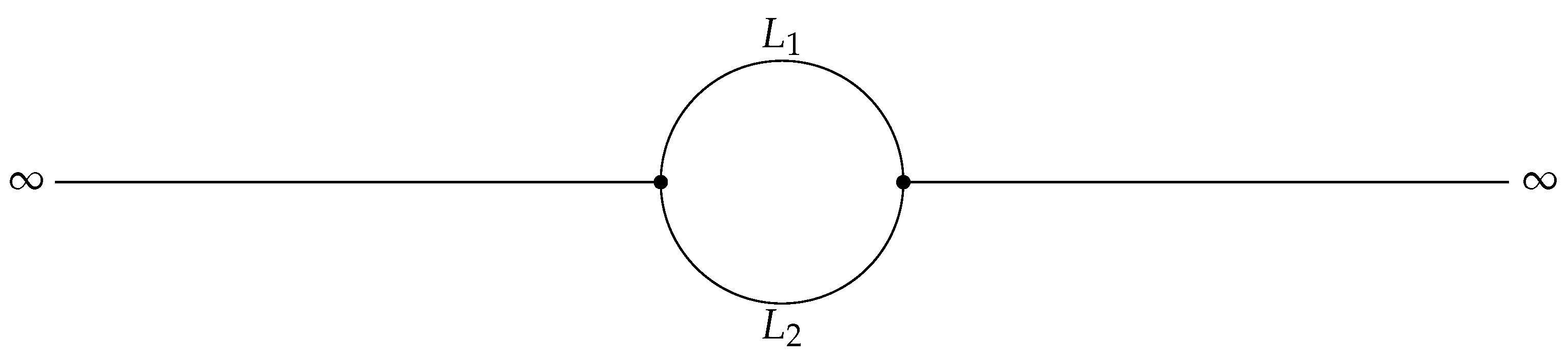
In this paper, we are interested in a special example, which reveals an unsuspectedly complex structure of the set of standing waves. More precisely, we consider a metric graph $\mathcal{G}$ made up of two half lines joined by two bounded edges, i.e., a so-called double-bridge graph (see Figure 1). $\mathcal{G}$ can also be thought of as a ring with two half lines attached in two distinct vertices. The half lines are both identified with the interval $[0,+\infty )$, while the bounded edges are represented by two bounded intervals of lengths $L_1>0$ and $L_2\ge L_1$, precisely $\left[0,L_1\right]$ and $[L_1,L]$ with $L=L_1+L_2$.

A function $\psi$ on $\mathcal{G}$ is a Cartesian product $\psi (x_1,\dots ,x_4)=({\psi }_1\left(x_1\right),\dots ,{\psi }_4\left(x_4\right))$ with $x_j\in I_j$ for $j=1,\dots ,4$, where $I_1=[0,L_1]$, $I_2=[L_1,L]$ and $I_3=I_4=[0,+\infty )$. Then, a Schrödinger operator $H_{\mathcal{G}}$ on $\mathcal{G}$ is defined as

$$H_{\mathcal{G}}\psi \left(x_1,\dots ,x_4\right)=\left(-{\psi }_1^{″}\left(x_1\right),\dots ,-{\psi }_4^{″}\left(x_4\right)\right),x_j\in I_j,$$

(1)

with domain $D\left(H_{\mathcal{G}}\right)$ given by the functions $\psi$ on $\mathcal{G}$ whose components satisfy ${\psi }_j\in H^2\left(I_j\right)$ together with the so-called Kirchhoff boundary conditions, i.e.,

$${\psi }_1\left(0\right)={\psi }_2\left(L\right)={\psi }_3\left(0\right),{\psi }_1\left(L_1\right)={\psi }_2\left(L_1\right)={\psi }_4\left(0\right),$$

(2)

$${\psi }_1^{\prime }\left(0\right)-{\psi }_2^{\prime }\left(L\right)+{\psi }_3^{\prime }\left(0\right)={\psi }_1^{\prime }\left(L_1\right)-{\psi }_2^{\prime }\left(L_1\right)-{\psi }_4^{\prime }\left(0\right)=0.$$

(3)

As is well known (see [14] for general information on quantum graphs), the operator $H_{\mathcal{G}}$ is self-adjoint on the domain $D\left(H_{\mathcal{G}}\right)$, and it generates a unitary Schrödinger dynamics. Essential information about its spectrum is given in ([15], Appendix A). We perturb this linear dynamics with a focusing cubic term, namely we consider the following NLS on $\mathcal{G}$

$$i\frac{d{\psi }_t}{dt}=H_{\mathcal{G}}{\psi }_t-{\left|{\psi }_t\right|}^2{\psi }_t$$

(4)

where the nonlinear term $|{\psi }_t{|}^2{\psi }_t$ is a shortened notation for $\left(\right|{\psi }_{1,t}{|}^2{\psi }_{1,t},\dots ,\left|{\psi }_{4,t}{|}^2{\psi }_{4,t}\right)$. Hence, Equation (4) is a system of scalar NLS equations on the intervals $I_j$ coupled through the Kirchhoff boundary conditions in Equations (2)–(3) included in the domain of $H_{\mathcal{G}}$. On rather general grounds, it can be shown that this problem enjoys well-posedness both in strong sense and in the energy space (see in particular ([2], Section 2.6)).

We are interested in standing waves of Equation (4), i.e., its solutions of the form ${\psi }_t=e^{-i\omega t}U\left(x\right)$ where $\omega \in \mathbb{R}$ and $U(x_1,\dots ,x_4)=(u_1\left(x_1\right),\dots ,u_4\left(x_4\right))$ is a purely spatial function on $\mathcal{G}$, which may also depend on $\omega$. Such a problem has already been considered in [11,12,15,16]. In particular, in [11,12], variational methods are used to show, among many other things, that Equation (4) has no ground state, i.e., no standing wave exists that minimizes the energy at fixed $L^2$-norm. In a recent paper [16], information on positive bound states that are not ground states is given. The special example of tadpole graph (a ring with a single half-line) is treated in detail in [17,18].

As for the results in [15], they can be summarized as follows. Writing the problem of standing waves of Equation (4) component-wise, we get the following scalar problem:

$$\left\{\begin{array}{cc}-u_j^{″}-u_j^3=\omega u_j,\hfill & u_j\in H^2\left(I_j\right)\hfill \\ u_1\left(0\right)=u_2\left(L\right)=u_3\left(0\right),\hfill & u_1\left(L_1\right)=u_2\left(L_1\right)=u_4\left(0\right)\hfill \\ u_1^{\prime }\left(0\right)-u_2^{\prime }\left(L\right)+u_3^{\prime }\left(0\right)=0,\hfill & u_1^{\prime }\left(L_1\right)-u_2^{\prime }\left(L_1\right)-u_4^{\prime }\left(0\right)=0.\hfill \end{array}\right.$$

(5)

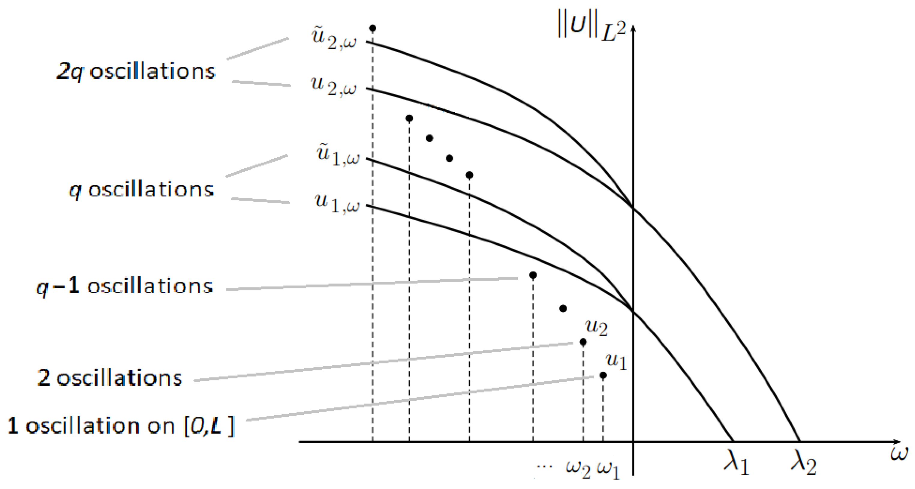
Such a system has solutions with $u_3=u_4=0$ if and only if the ratio $L_1/L_2$ is rational. In this case, they form a sequence of continuous branches in the $\left(\omega ,{∥U∥}_{L^2}\right)$ plane, bifurcating from the linear eigenvectors of the Schrödinger operator $H_{\mathcal{G}}$ (see Figure 2), and they are periodic on the ring of $\mathcal{G}$, that is, $u_1$ and $u_2$ are restrictions to $I_1$ and $I_2$ of a function u belonging to the second Sobolev space of periodic functions $H_{\mathrm{per}}^2\left([0,L]\right)=\left\{u\in H^2\left([0,L]\right):u\left(0\right)=u\left(L\right),u^{\prime }\left(0\right)=u^{\prime }\left(L\right)\right\}$. In particular, such function u is a rescaled Jacobi cnoidal function (see, e.g., [19,20] for a treatise on the Jacobian elliptic functions). If $\omega \ge 0$, no other nonzero standing waves exist, since the NLS on the unbounded edges has no nontrivial solution. If $\omega <0$, instead, the NLS on the half lines has soliton solutions, so that standing waves with nonzero $u_3$ and $u_4$ are admissible. The general study of this kind of solutions leads to a rather complicated system of equations, since, while $u_3$ and $u_4$ must be shifted solitons, each of $u_1$ and $u_2$ can be (at least in principle) a cnoidal function, a dnoidal function or a shifted soliton. To limit this complexity, the analysis in [15] is focused on the special case of standing waves that are non-vanishing on the half lines but share the above-mentioned periodicity feature with the bifurcation solutions. This amounts to study the following system:

$$\left\{\begin{array}{cc}-u^{″}-u^3=\omega u,\hfill & u\in H_{\mathrm{per}}^2\left([0,L]\right),\omega <0\hfill \\ u\left(0\right)=\pm u\left(L_1\right)=\sqrt{2\left|\omega \right|}\hfill \end{array}\right.$$

(6)

where the sign ± distinguishes the cases of $u_3$ and $u_4$ with the same sign (which we may assume positive, thanks to the odd parity of the equation) or with different signs. In [15], it is shown that:

(i)

If $L_1/L_2\in \mathbb{Q}$, then the set of solutions to (6) is made up of a sequence of secondary bifurcation branches ${\left\{(\omega ,{\tilde{u}}_{n,\omega }):\omega <0\right\}}_{n\ge 1}$, originating at $\omega =0$ from each of the previous ones, together with a sequence ${\left\{\left({\omega }_n,u_n\right)\right\}}_{n\ge 1}$ not lying on any branch (see Figure 2).

(ii)

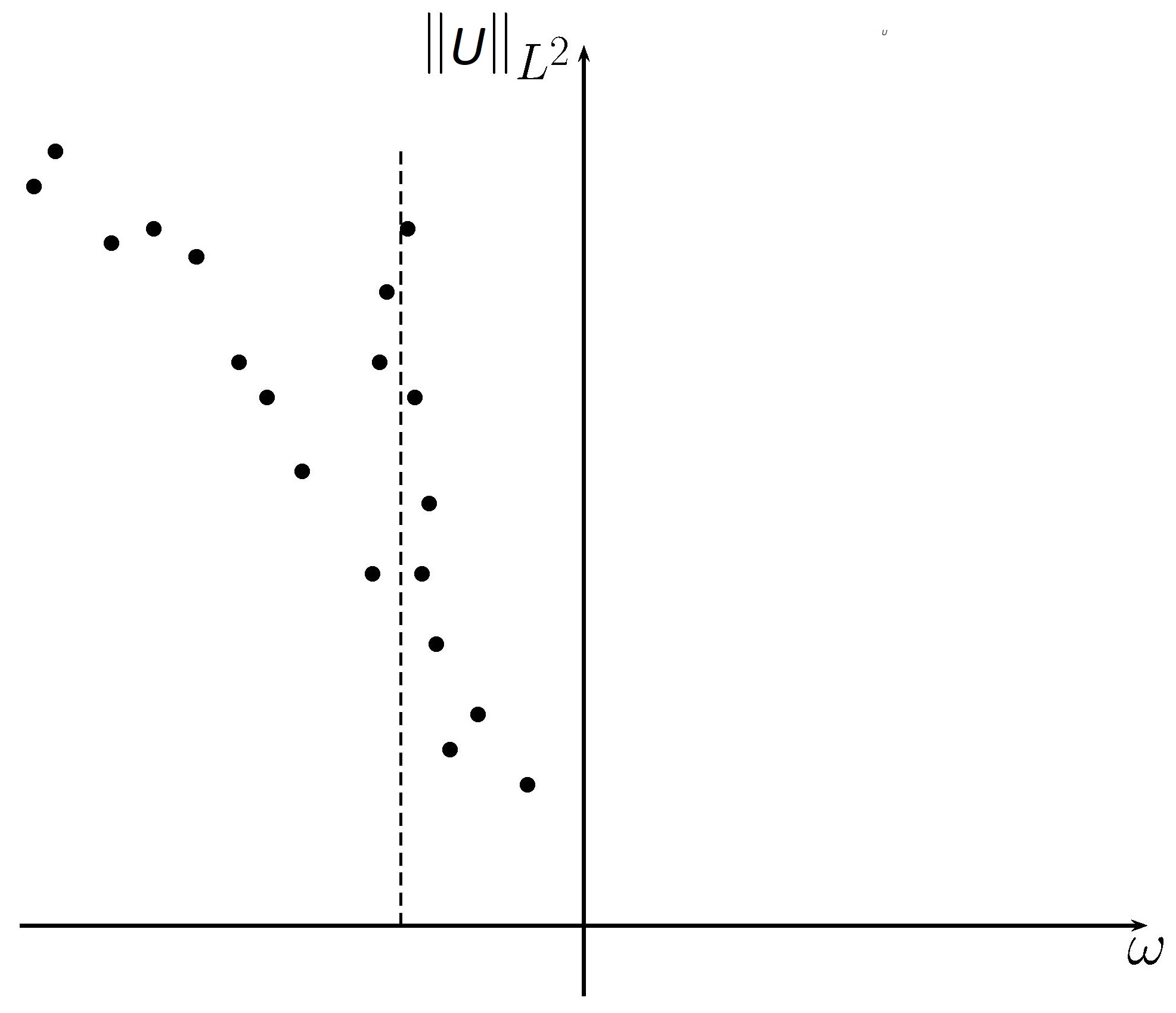
If $L_1/L_2\notin \mathbb{Q}$, then the set of solutions to (6) reduces to two sequences ${\left\{\left({\omega }_n^{+},u_n^{+}\right)\right\}}_{n\ge 1}$ and ${\left\{\left({\omega }_n^{-},u_n^{-}\right)\right\}}_{n\ge 1}$ alone, solving the problem in Equation (6) with sign ±, respectively, where the frequency sequences ${\left\{{\omega }_n^{\pm }\right\}}_{n\ge 1}$ are unbounded below and have at least a finite nonzero cluster point (see Figure 3). The functions $u_n^{\pm }$ oscillate n times on the ring of the graph.

These results come rather unexpectedly, so the aim of this paper is to pursue the study begun in [15] by deepening the understanding of such results in relation to the underlying physical model. In particular, we ask the following questions: Does Equation (4) admit standing waves that are non-periodic on ring of $\mathcal{G}$? If so, do they form continuous branches to which the isolated periodic solutions belong?

With a view to especially answer the second question, we look for standing waves which include the ones given by Equation (6) but still change sign on the bounded edges. More precisely, we look for solutions to Equation (5) exhibiting the following features:

• $u_1,u_2$ are sign-changing.
• $u_3,u_4$ are nonzero.

The second feature implies $\omega <0$ and

$$u_j\left(x\right)=\pm \sqrt{2}\eta \mathrm{sech}\left(\eta \left(x+a_j\right)\right),a_j\in \mathbb{R},j=3,4$$

(7)

where we set $\eta :=\sqrt{\left|\omega \right|}$ for brevity. Then, the first feature implies

$$u_j\left(x\right)=\eta \sqrt{\frac{2k_j^2}{2k_j^2-1}}\mathrm{cn}\left(\frac{\eta }{\sqrt{2k_j^2-1}}\left(x+a_j\right);k_j\right),k_j\in \left(\frac{1}{\sqrt{2}},1\right),a_j\in \left[0,T_j\right),j=1,2$$

(8)

where $\mathrm{cn}\left(·;k\right)$ is the cnoidal function of parameter k and $T_j=T_j\left(k_j,\eta \right):=S\left(k_j\right)/\eta$ is the period of the function $\mathrm{cn}\left(\eta \left(·\right)/\sqrt{2k_j^2-1};k_j\right)$. Here and in the rest of the paper, S denotes the function

$$S\left(k\right):=4\sqrt{2k^2-1}K\left(k\right)=4\sqrt{2k^2-1}{\int }_0^1\frac{dt}{\sqrt{\phantom{(}(1-t^2)(1-k^2{t}^2)}},$$

(9)

where $K\left(k\right)$ is the so called complete elliptic integral of first kind. Notice that $S:(1/\sqrt{2},1)\to \mathbb{R}$ is strictly increasing, continuous and such that $S\left((1/\sqrt{2},1)\right)=\left(0,+\infty \right)$.

Therefore, restricting ourselves for simplicity to the case with $u_3$ and $u_4$ of the same sign, which we may assume positive thanks to the odd parity of the system in Equation (5), we are led to study the existence of solutions $\eta >0$, $k_1,k_2\in \left(\frac{1}{\sqrt{2}},1\right)$, $a_1\in \left[0,T_1\right)$, $a_2\in \left[0,T_2\right)$, $a_3,a_4\in \mathbb{R}$ to the following system:   

$$\left\{\begin{array}{c}\frac{k_1}{\sqrt{2k_1^2-1}}\mathrm{cn}\left(\frac{\eta a_1}{\sqrt{2k_1^2-1}};k_1\right)=\frac{k_2}{\sqrt{2k_2^2-1}}\mathrm{cn}\left(\frac{\eta \left(L+a_2\right)}{\sqrt{2k_2^2-1}};k_2\right)=\mathrm{sech}\left(\eta a_3\right)\hfill \\ \frac{k_1}{\sqrt{2k_1^2-1}}\mathrm{cn}\left(\frac{\eta \left(L_1+a_1\right)}{\sqrt{2k_1^2-1}};k_1\right)=\frac{k_2}{\sqrt{2k_2^2-1}}\mathrm{cn}\left(\frac{\eta \left(L_1+a_2\right)}{\sqrt{2k_2^2-1}};k_2\right)=\mathrm{sech}\left(\eta a_4\right)\hfill \\ \tanh \left(\eta a_3\right)\mathrm{sech}\left(\eta a_3\right)=\hfill \\ =-\frac{k_1}{2k_1^2-1}\mathrm{sn}\left(\frac{\eta a_1}{\sqrt{2k_1^2-1}};k_1\right)\mathrm{dn}\left(\frac{\eta a_1}{\sqrt{2k_1^2-1}};k_1\right)+\frac{k_2}{2k_2^2-1}\mathrm{sn}\left(\frac{\eta \left(L+a_2\right)}{\sqrt{2k_2^2-1}};k_2\right)\mathrm{dn}\left(\frac{\eta \left(L+a_2\right)}{\sqrt{2k_2^2-1}};k_2\right)\hfill \\ \tanh \left(\eta a_4\right)\mathrm{sech}\left(\eta a_4\right)=\hfill \\ =\frac{k_1}{2k_1^2-1}\mathrm{sn}\left(\frac{\eta \left(L_1+a_1\right)}{\sqrt{2k_1^2-1}};k_1\right)\mathrm{dn}\left(\frac{\eta \left(L_1+a_1\right)}{\sqrt{2k_1^2-1}};k_1\right)-\frac{k_2}{2k_2^2-1}\mathrm{sn}\left(\frac{\eta \left(L_1+a_2\right)}{\sqrt{2k_2^2-1}};k_2\right)\mathrm{dn}\left(\frac{\eta \left(L_1+a_2\right)}{\sqrt{2k_2^2-1}};k_2\right).\hfill \end{array}\right.$$

(10)

This set of equations turns out to be still rather difficult to study in his full generality, and indeed we have results only in the subcase where the two solitons in Equation (7) have the same height at the vertices, i.e., $\mathrm{sech}\left(\eta a_3\right)=\mathrm{sech}\left(\eta a_4\right)$ (which corresponds to ${\theta }_1={\theta }_2$ in Section 2). More precisely, in Section 2 we reduce the system in Equation (10) to an equivalent one, which naturally splits into different cases. Then, we study three of such cases, all with $\mathrm{sech}\left(\eta a_3\right)=\mathrm{sech}\left(\eta a_4\right)$, leading to our existence results, which are the following three theorems.

The first two results only concern the case of irrational ratios $L_1/L_2$ and give solutions with $k_1\ne k_2$, i.e., non-periodic on the ring of the graph.

Theorem 1.

Assume that $L_1/L_2\in \mathbb{R}\backslash \mathbb{Q}$. Then, there exists a sequence of positive integers ${\left(n_h\right)}_{h\in \mathbb{N}}$ such that for every $\omega <-32K{(1/\sqrt{2})}^2/\left(L_1{L}_2\right)$ there exists $h_{\omega }\in \mathbb{N}$ (also depending on $L_1$ and $L_2$) such that for all $h>h_{\omega }$ the problem in Equation (5) has two solutions $(u_{1,h}^{+},u_{2,h}^{+},u_{3,h}^{+},u_{4,h}^{+})$ and $(u_{1,h}^{-},u_{2,h}^{-},u_{3,h}^{-},u_{4,h}^{-})$ of the form:

$$u_{j,h}^{\pm }\left(x\right)=\sqrt{\frac{2\left|\omega \right|k_{j,h}^2}{2k_{j,h}^2-1}}\mathrm{cn}\left(\sqrt{\frac{\left|\omega \right|}{2k_{j,h}^2-1}}\left(x+a_{j,h}^{\pm }\right);k_{j,h}\right),j=1,2$$

(11)

$$u_{j,h}^{\pm }\left(x\right)=\sqrt{2\left|\omega \right|}\mathrm{sech}\left(\sqrt{\left|\omega \right|}\left(x+a_{j,h}^{\pm }\right)\right),j=3,4$$

(12)

where $u_{1,h}^{\pm }\left(x\right)$ and $u_{2,h}^{\pm }\left(x\right)$ have periods $T_{1,h}=L_1/\left[n_h{L}_1/L_2+1\right]$ and $T_{2,h}=L_2/n_h$, and for all h one has

$$\frac{1}{\sqrt{2}}<k_{1,h}<k_{2,h}<1,a_{1,h}^{\pm }\in \left(0,\frac{T_{1,h}}{4}\right),a_{2,h}^{\pm }\in \left[0,T_{2,h}\right),a_{3,h}^{\pm }<0,a_{4,h}^{\pm }>0,a_{j,h}^{+}\ne a_{j,h}^{-}.$$

(13)

Remark 1.

More precisely, according to the proof, in Theorem 1, we have that

$$\begin{array}{c}{k}_{1,h}=S^{-1}\left(\frac{L_1}{\left[n_h{L}_1/L_2+1\right]}\sqrt{\left|\omega \right|}\right),a_{1,h}^{\pm }={\gamma }_1(k_{1,h},\omega ,{\theta }_h^{\pm }),\hfill \\ k_{2,h}=S^{-1}\left(\frac{L_2}{n_h}\sqrt{\left|\omega \right|}\right),a_{2,h}^{\pm }={\gamma }_2(k_{2,h},\omega ,{\theta }_h^{\pm })-L+p{T}_{2,h},-a_{3,h}^{\pm }=a_{4,h}^{\pm }={\mathrm{sech}}_{\mid \left[0,+\infty \right)}^{-1}\left({\theta }_h^{\pm }\right),\hfill \end{array}$$

where p is the unique positive integer such that $a_{2,h}^{\pm }\in \left[0,T_{2,h}\right)$, ${\theta }_h^{\pm }$ are the two distinct solutions in $\left(0,1\right]$ of the equation ${\theta }^2\left(1-{\theta }^2\right)=t_{k_{1,h},k_{2,h}}$ with $t_{k_{1,h},k_{2,h}}$ given by Equation (17), and ${\gamma }_j(k_{j,h},\omega ,{\theta }_h^{\pm })$ is the unique preimage in $\left(0,T_{j,h}/4\right)$ of ${\theta }_h^{\pm }\sqrt{2k_{j,h}^2-1}/k_{j,h}$ by the function $\mathrm{cn}\left(\left(·\right)\sqrt{\left|\omega \right|}/\sqrt{2k_{j,h}^2-1};k_{j,h}\right)$.

Theorem 2.

Assume that $L_1/L_2\in \mathbb{R}\backslash \mathbb{Q}$. Then, there exists a sequence of positive integers ${\left(n_h\right)}_{h\in \mathbb{N}}$ such that for every $\omega <-32K{(1/\sqrt{2})}^2/\left(L_1{L}_2\right)$ there exists $h_{\omega }\in \mathbb{N}$ (also depending on $L_1$ and $L_2$) such that for all $h>h_{\omega }$ the problem in Equation (5) has two solutions $(u_{1,h}^{\pm },u_{2,h}^{\pm },u_{3,h}^{\pm },u_{4,h}^{\pm })$ of the form of Equations (11)–(12), where $u_{1,h}^{\pm }\left(x\right)$ and $u_{2,h}^{\pm }\left(x\right)$ have periods $T_{1,h}=L_1/\left[n_h{L}_1/L_2\right]$ and $T_{2,h}=L_2/n_h$, the parameters $a_{1,h}^{\pm },a_{2,h}^{\pm },a_{3,h}^{\pm },a_{4,h}^{\pm }$ are as in Equation (13) and for all h one has   

$$\frac{1}{\sqrt{2}}<k_{2,h}<k_{1,h}<1.$$

Remark 2.

More precisely, in Theorem 2 we have that

$$k_{1,h}=S^{-1}\left(\frac{L_1}{\left[n_h{L}_1/L_2\right]}\sqrt{\left|\omega \right|}\right)\mathit{and}{k}_{2,h}=S^{-1}\left(\frac{L_2}{n_h}\sqrt{\left|\omega \right|}\right),$$

whereas $a_{j,h}^{\pm }$ are exactly as in Remark 1.

The third result does not need $L_1/L_2$ irrational and concerns the subcase of the system in Equation (5) which, if $L_1/L_2\in \mathbb{R}\backslash \mathbb{Q}$ and $k_1=k_2$, is exactly the system in Equation (6) with plus sign (see Remark 5).

Theorem 3.

Let $m,n\in \mathbb{N}$ be such that $n>m\ge 1$. Then, there exists ${\omega }_{m,n}<0$ (also depending on $L_1$) such that for all $\omega <{\omega }_{m,n}$ the problem in Equation (5) has a solution $\left(u_1,u_2,u_3,u_4\right)$ of the form of Equations (7)–(8), with $k_1,k_2\in \left(\sqrt{3}/2,1\right)$, $a_1\in \left(0,T_1/4\right)$, $a_2\in \left[0,T_2\right)$.

Remark 3.

According to the proof, in Theorem 3, $a_1,a_2,a_3,a_4$ can be described in a similar way of Theorems 1 and 2. On the contrary, the parameters $k_1,k_2$ do exist, but are not explicit as in the previous theorems.

As already mentioned, Theorems 1–3 do not exhaust the study of solutions to the problem in Equation (5), and thus of standing waves of (NLS), as they only concern the case of solitons having the same height at the vertices. In addition, they do not describe the whole family of this kind of solutions, but only give existence results. However, they still provide some answer to the questions raised above. Indeed, Theorems 1 and 2 answer in the affirmative to the first question, as they prove existence of standing waves which are non-periodic on the ring of $\mathcal{G}$. As to Theorem 3, for any m and n, it provides a family of solutions which depend on the continuous parameter $\omega \in (-\infty ,{\omega }_{m,n})$ and, roughly speaking, make m oscillations on the edge of length $L_1$ and $n-m$ oscillations on the one of length $L_2$ (cf. the second and third equations of the system in Equation (33)). If $L_1/L_2$ is irrational and one of these families contain a solution with $k_1=k_2$, then such a solution is one of the isolated solutions found in [15] in the irrational case and we can answer affirmatively also to the second question. Unfortunately, the argument we used in proving Theorem 3 does not allow us to say wether we find solutions with $k_1=k_2$ or not, and therefore we do not have a final answer to the second question.

2. Preliminaries

In this section, we reduce the system in Equation (10) to a simpler equivalent one, which is the system in Equation (14) with the last two equations replaced by the system in Equation (19).

For brevity, we set

$$X_1=\frac{\eta a_1}{\sqrt{2k_1^2-1}},X_2=\frac{\eta \left(L+a_2\right)}{\sqrt{2k_2^2-1}},X_3=\frac{\eta \left(L_1+a_1\right)}{\sqrt{2k_1^2-1}},X_4=\frac{\eta \left(L_1+a_2\right)}{\sqrt{2k_2^2-1}},$$

and

$${\sigma }_1=\mathrm{sgn}\left[\mathrm{sn}\left(X_1;k_1\right)\right],{\sigma }_2=\mathrm{sgn}\left[\mathrm{sn}\left(X_2;k_2\right)\right],{\sigma }_3=\mathrm{sgn}\left[\mathrm{sn}\left(X_3;k_1\right)\right],{\sigma }_4=\mathrm{sgn}\left[\mathrm{sn}\left(X_4;k_2\right)\right].$$

Then, using well known identities (see [20]) and the first equation of the system in Equation (10), we get   

$$\begin{array}{ccc}\hfill \mathrm{sn}\left(X_1;k_1\right)& =& {\sigma }_1\sqrt{1-{\mathrm{cn}}^2\left(X_1;k_1\right)}={\sigma }_1\sqrt{1-\frac{2k_1^2-1}{k_1^2}{\mathrm{sech}}^2\left(\eta a_3\right)},\hfill \\ \hfill \mathrm{dn}\left(X_1;k_1\right)& =& \sqrt{1-k_1^2+k_1^2{\mathrm{cn}}^2\left(X_1;k_1\right)}=\sqrt{1-k_1^2+\left(2k_1^2-1\right){\mathrm{sech}}^2\left(\eta a_3\right)}\hfill \end{array}$$

and hence

$$\begin{array}{ccc}\frac{k_1}{2k_1^2-1}\mathrm{sn}\left(X_1;k_1\right)\mathrm{dn}\left(X_1;k_1\right)\hfill & =& {\sigma }_1\sqrt{\frac{k_1^2}{2k_1^2-1}-{\mathrm{sech}}^2\left(\eta a_3\right)}\sqrt{\frac{\left(1-k_1^2\right)}{2k_1^2-1}+{\mathrm{sech}}^2\left(\eta a_3\right)}\hfill \\ & =& {\sigma }_1\sqrt{\frac{k_1^2\left(1-k_1^2\right)}{{\left(2k_1^2-1\right)}^2}+{\mathrm{sech}}^2\left(\eta a_3\right)-{\mathrm{sech}}^4\left(\eta a_3\right)}.\hfill \end{array}$$

Arguing similarly for the products $\mathrm{sn}\left(X_2;k_2\right)\mathrm{dn}\left(X_2;k_2\right)$, $\mathrm{sn}\left(X_3;k_1\right)\mathrm{dn}\left(X_3;k_1\right)$ and $\mathrm{sn}\left(X_4;k_2\right)\mathrm{dn}\left(X_4;k_2\right)$, and defining

$$c\left(k\right):=\frac{k^2\left(1-k^2\right)}{{\left(2k^2-1\right)}^2},$$

we thus obtain that the system in Equation (10) is equivalent to

$$\left\{\begin{array}{c}\frac{k_1}{\sqrt{2k_1^2-1}}\mathrm{cn}\left(\frac{\eta a_1}{\sqrt{2k_1^2-1}};k_1\right)=\frac{k_2}{\sqrt{2k_2^2-1}}\mathrm{cn}\left(\frac{\eta \left(L+a_2\right)}{\sqrt{2k_2^2-1}};k_2\right)=\mathrm{sech}\left(\eta a_3\right)\hfill \\ \frac{k_1}{\sqrt{2k_1^2-1}}\mathrm{cn}\left(\frac{\eta \left(L_1+a_1\right)}{\sqrt{2k_1^2-1}};k_1\right)=\frac{k_2}{\sqrt{2k_2^2-1}}\mathrm{cn}\left(\frac{\eta \left(L_1+a_2\right)}{\sqrt{2k_2^2-1}};k_2\right)=\mathrm{sech}\left(\eta a_4\right)\hfill \\ \tanh \left(\eta a_3\right)\mathrm{sech}\left(\eta a_3\right)=-{\sigma }_1\sqrt{c\left(k_1\right)+{\mathrm{sech}}^2\left(\eta a_3\right)-{\mathrm{sech}}^4\left(\eta a_3\right)}+{\sigma }_2\sqrt{c\left(k_2\right)+{\mathrm{sech}}^2\left(\eta a_3\right)-{\mathrm{sech}}^4\left(\eta a_3\right)}\hfill \\ \tanh \left(\eta a_4\right)\mathrm{sech}\left(\eta a_4\right)={\sigma }_3\sqrt{c\left(k_1\right)+{\mathrm{sech}}^2\left(\eta a_4\right)-{\mathrm{sech}}^4\left(\eta a_4\right)}-{\sigma }_4\sqrt{c\left(k_2\right)+{\mathrm{sech}}^2\left(\eta a_4\right)-{\mathrm{sech}}^4\left(\eta a_4\right)}.\hfill \end{array}\right.$$

(14)

Let us now focus on the last two equations. Setting

$${\theta }_1=\mathrm{sech}\left(\eta a_3\right),{\theta }_2=\mathrm{sech}\left(\eta a_4\right),{\sigma }_5=\mathrm{sgn}\left(a_3\right)=\mathrm{sgn}\left(\tanh \left(\eta a_3\right)\right),{\sigma }_6=\mathrm{sgn}\left(a_4\right)=\mathrm{sgn}\left(\tanh \left(\eta a_4\right)\right)$$

the couple of such equations is equivalent to

$$\left\{\begin{array}{c}{\sigma }_5\sqrt{1-{\theta }_1^2}{\theta }_1=-{\sigma }_1\sqrt{c\left(k_1\right)+{\theta }_1^2\left(1-{\theta }_1^2\right)}+{\sigma }_2\sqrt{c\left(k_2\right)+{\theta }_1^2\left(1-{\theta }_1^2\right)}\hfill \\ {\sigma }_6\sqrt{1-{\theta }_2^2}{\theta }_2={\sigma }_3\sqrt{c\left(k_1\right)+{\theta }_2^2\left(1-{\theta }_2^2\right)}-{\sigma }_4\sqrt{c\left(k_2\right)+{\theta }_2^2\left(1-{\theta }_2^2\right)}.\hfill \end{array}\right.$$

(15)

Squaring the equations, we get

$$c\left(k_1\right)+{\theta }_1^2\left(1-{\theta }_1^2\right)+c\left(k_2\right)-2{\sigma }_1{\sigma }_2\sqrt{c\left(k_1\right)+{\theta }_1^2\left(1-{\theta }_1^2\right)}\sqrt{c\left(k_2\right)+{\theta }_1^2\left(1-{\theta }_1^2\right)}=0,$$

$$c\left(k_1\right)+{\theta }_2^2\left(1-{\theta }_2^2\right)+c\left(k_2\right)-2{\sigma }_3{\sigma }_4\sqrt{c\left(k_1\right)+{\theta }_2^2\left(1-{\theta }_2^2\right)}\sqrt{c\left(k_2\right)+{\theta }_2^2\left(1-{\theta }_2^2\right)}=0,$$

which are impossible if ${\sigma }_1{\sigma }_2=-1$ or ${\sigma }_3{\sigma }_4=-1$. Hence, we can add the conditions ${\sigma }_1={\sigma }_2$ and ${\sigma }_3={\sigma }_4$ to the system in Equation (15), and get

$$\left\{\begin{array}{c}{\sigma }_5\sqrt{1-{\theta }_1^2}{\theta }_1={\sigma }_1\left(-\sqrt{c\left(k_1\right)+{\theta }_1^2\left(1-{\theta }_1^2\right)}+\sqrt{c\left(k_2\right)+{\theta }_1^2\left(1-{\theta }_1^2\right)}\right)\hfill \\ {\sigma }_6\sqrt{1-{\theta }_2^2}{\theta }_2={\sigma }_3\left(\sqrt{c\left(k_1\right)+{\theta }_2^2\left(1-{\theta }_2^2\right)}-\sqrt{c\left(k_2\right)+{\theta }_2^2\left(1-{\theta }_2^2\right)}\right)\hfill \\ {\sigma }_2={\sigma }_1,{\sigma }_4={\sigma }_3.\hfill \end{array}\right.$$

(16)

Moreover, both ${\theta }_1^2\left(1-{\theta }_1^2\right)$ and ${\theta }_2^2\left(1-{\theta }_2^2\right)$ must be solutions $t\in \left[0,1/4\right]$ of the equation

$$c\left(k_1\right)+c\left(k_2\right)+t-2\sqrt{c\left(k_1\right)+t}\sqrt{c\left(k_2\right)+t}=0.$$

Such equation has the unique nonnegative solution

$$t=t_{k_1,k_2}=\frac{1}{3}\left(2\sqrt{c{\left(k_1\right)}^2-c\left(k_1\right)c\left(k_2\right)+c{\left(k_2\right)}^2}-c\left(k_1\right)-c\left(k_2\right)\right),$$

(17)

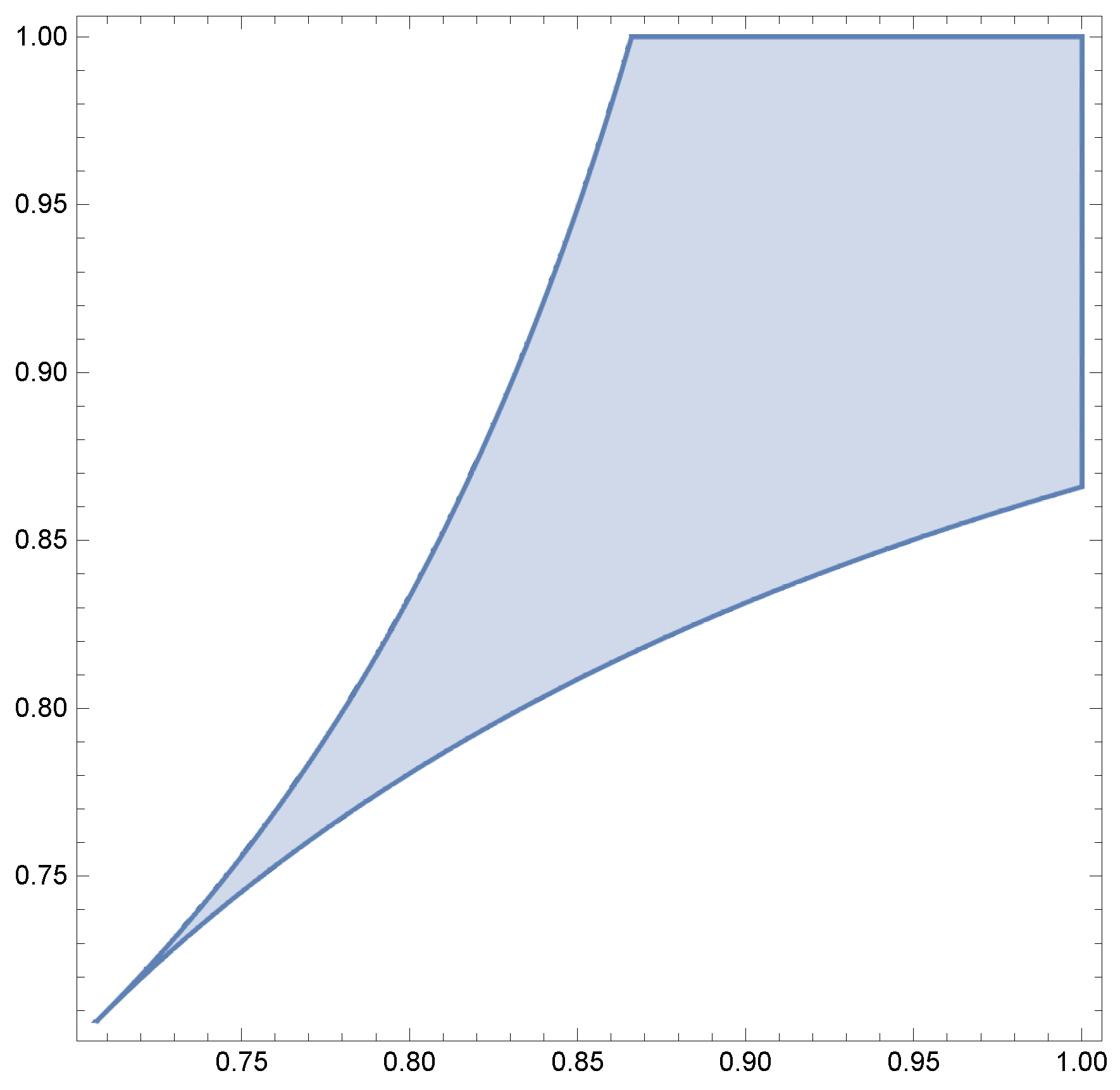
which belongs to $\left[0,1/4\right]$ if and only if $\left(k_1,k_2\right)$ belongs to the set

$$A=\left\{\left(k_1,k_2\right)\in {\left(\frac{1}{\sqrt{2}},1\right)}^2:2\sqrt{c{\left(k_1\right)}^2-c\left(k_1\right)c\left(k_2\right)+c{\left(k_2\right)}^2}-c\left(k_1\right)-c\left(k_2\right)\le \frac{3}{4}\right\},$$

i.e., as one can easily see after some computations,

$$A=\left\{\left(k_1,k_2\right)\in \mathbb{R}:k_1\in \left(\frac{1}{\sqrt{2}},1\right),\frac{\sqrt{4k_1^2-1}}{2k_1}\le k_2\le \frac{1}{2\sqrt{1-k_1^2}},k_2<1\right\}$$

(the set A is portrayed in Figure 4).

In this case, the equation ${\theta }^2\left(1-{\theta }^2\right)=t_{k_1,k_2}$ with $\theta \in \left(0,1\right]$ has two distinct solutions

$${\theta }_{k_1,k_2}^{\pm }=\sqrt{\frac{1\pm \sqrt{1-4t_{k_1,k_2}}}{2}}$$

(18)

if $t_{k_1,k_2}\in \left(0,1/4\right)$, two coincident solutions ${\theta }_{k_1,k_2}^{+}={\theta }_{k_1,k_2}^{-}=1/\sqrt{2}$ if $t_{k_1,k_2}=1/4$, and a unique solution ${\theta }_{k_1,k_2}^{+}=1$ if $t_{k_1,k_2}=0$ (i.e., $k_1=k_2$). In this latter case, we still write ${\theta }_{k_1,k_2}^{+}={\theta }_{k_1,k_2}^{-}=1$ for future convenience. We also observe that the function $c\left(k\right)$ is positive and strictly decreasing from $\left(1/\sqrt{2},1\right)$ onto $\left(0,+\infty \right)$, so that the terms within brackets on the right hand sides of the first two equations of Equation (16) have a fixed sign according as $k_1<k_2$ or $k_1>k_2$. Therefore, the system in Equation (15) turns out to be equivalent to

$$\left\{\begin{array}{c}\left(k_1,k_2\right)\in A,{\theta }_1,{\theta }_2\in \left\{{\theta }_{k_1,k_2}^{+},{\theta }_{k_1,k_2}^{-}\right\}\hfill \\ \mathrm{sech}\left(\eta a_3\right)={\theta }_1,\mathrm{sech}\left(\eta a_4\right)={\theta }_2\hfill \\ \left\{\begin{array}{c}{k}_1<k_2\hfill \\ {\sigma }_5=-{\sigma }_1\hfill \\ {\sigma }_6={\sigma }_3\hfill \end{array}\right.\vee \left\{\begin{array}{c}{k}_1>k_2\hfill \\ {\sigma }_5={\sigma }_1\hfill \\ {\sigma }_6=-{\sigma }_3\hfill \end{array}\right.\vee \left\{\begin{array}{c}{k}_1=k_2\hfill \\ a_3=a_4=0\hfill \end{array}\right.\hfill \\ {\sigma }_2={\sigma }_1,{\sigma }_4={\sigma }_3.\hfill \end{array}\right.$$

(19)

As a conclusion, Equation (10) is equivalent to the system in Equation (14) with the last two equations replaced by the system in Equation (19).

3. Case ${\mathit{\theta }}_{\mathbf{1}}={\mathit{\theta }}_{\mathbf{2}}$, ${\mathit{\sigma }}_{\mathbf{1}}={\mathit{\sigma }}_{\mathbf{3}}$ and ${\mathit{k}}_{\mathbf{1}}<{\mathit{k}}_{\mathbf{2}}$. Proof of Theorem 1

We focus on the case ${\sigma }_1={\sigma }_3=1$, which gives Theorem 1, leaving the analogous case ${\sigma }_1={\sigma }_3=-1$ to the interested reader. In such a case, condition $\left(k_1,k_2\right)\in A$ becomes

$$\left(k_1,k_2\right)\in A^{\prime }=A\cap \left\{\left(k_1,k_2\right)\in \mathbb{R}:k_1<k_2\right\}=\left\{\left(k_1,k_2\right)\in \mathbb{R}:\frac{1}{\sqrt{2}}<k_1<k_2\le \frac{1}{2\sqrt{1-k_1^2}},k_2<1\right\}$$

and, taking into account the equivalence between Equation (15) and Equation (19), the system in Equation (14) becomes:

$$\left\{\begin{array}{c}\left(k_1,k_2\right)\in A^{\prime },\theta \in \left\{{\theta }_{k_1,k_2}^{+},{\theta }_{k_1,k_2}^{-}\right\}\hfill \\ \mathrm{sech}\left(\eta a_3\right)=\mathrm{sech}\left(\eta a_4\right)=\theta ,a_3<0,a_4>0\hfill \\ \frac{k_1}{\sqrt{2k_1^2-1}}\mathrm{cn}\left(\frac{\eta a_1}{\sqrt{2k_1^2-1}};k_1\right)=\frac{k_2}{\sqrt{2k_2^2-1}}\mathrm{cn}\left(\frac{\eta \left(L+a_2\right)}{\sqrt{2k_2^2-1}};k_2\right)=\theta \hfill \\ \frac{k_1}{\sqrt{2k_1^2-1}}\mathrm{cn}\left(\frac{\eta \left(L_1+a_1\right)}{\sqrt{2k_1^2-1}};k_1\right)=\frac{k_2}{\sqrt{2k_2^2-1}}\mathrm{cn}\left(\frac{\eta \left(L_1+a_2\right)}{\sqrt{2k_2^2-1}};k_2\right)=\theta \hfill \\ \mathrm{sn}\left(\frac{\eta a_1}{\sqrt{2k_1^2-1}};k_1\right)>0,\mathrm{sn}\left(\frac{\eta \left(L_1+a_1\right)}{\sqrt{2k_1^2-1}};k_1\right)>0\hfill \\ \mathrm{sn}\left(\frac{\eta \left(L+a_2\right)}{\sqrt{2k_2^2-1}};k_2\right)>0,\mathrm{sn}\left(\frac{\eta \left(L_1+a_2\right)}{\sqrt{2k_2^2-1}};k_2\right)>0.\hfill \end{array}\right.$$

(20)

We denote by ${\gamma }_j={\gamma }_j\left(k_j,\eta ,\theta \right)$ the unique preimage in $\left(0,T_j/4\right)$ of the value $\frac{\sqrt{2k_j^2-1}}{k_j}\theta$ by the function $\mathrm{cn}\left(\frac{\eta }{\sqrt{2k_j^2-1}}\left(·\right);k_j\right)$. Then,

$$\left\{\begin{array}{c}\frac{k_1}{\sqrt{2k_1^2-1}}\mathrm{cn}\left(\frac{\eta a_1}{\sqrt{2k_1^2-1}};k_1\right)=\theta ,\mathrm{sn}\left(\frac{\eta a_1}{\sqrt{2k_1^2-1}};k_1\right)>0\hfill \\ \frac{k_1}{\sqrt{2k_1^2-1}}\mathrm{cn}\left(\frac{\eta \left(L_1+a_1\right)}{\sqrt{2k_1^2-1}};k_1\right)=\theta ,\mathrm{sn}\left(\frac{\eta \left(L_1+a_1\right)}{\sqrt{2k_1^2-1}};k_1\right)>0\hfill \end{array}\right.$$

means

$$\left\{\begin{array}{c}{a}_1={\gamma }_1\hfill \\ L_1+a_1={\gamma }_1+m{T}_1\mathrm{for}\mathrm{some}m\ge 1,\hfill \end{array}\right.\mathrm{i}.\mathrm{e}.,\left\{\begin{array}{c}{a}_1={\gamma }_1\hfill \\ L_1=m{T}_1\mathrm{for}\mathrm{some}m\ge 1\hfill \end{array}\right.$$

while

$$\left\{\begin{array}{c}\frac{k_2}{\sqrt{2k_2^2-1}}\mathrm{cn}\left(\frac{\eta \left(L+a_2\right)}{\sqrt{2k_2^2-1}};k_2\right)=\theta ,\mathrm{sn}\left(\frac{\eta \left(L+a_2\right)}{\sqrt{2k_2^2-1}};k_2\right)>0\hfill \\ \frac{k_2}{\sqrt{2k_2^2-1}}\mathrm{cn}\left(\frac{\eta \left(L_1+a_2\right)}{\sqrt{2k_2^2-1}};k_2\right)=\theta ,\mathrm{sn}\left(\frac{\eta \left(L_1+a_2\right)}{\sqrt{2k_2^2-1}};k_2\right)>0\hfill \end{array}\right.$$

means

$$\left\{\begin{array}{c}L+a_2={\gamma }_2+p{T}_2\mathrm{for}\mathrm{some}p\ge 0\hfill \\ L_1+a_2={\gamma }_2+q{T}_2\mathrm{for}\mathrm{some}0\le q<p,\hfill \end{array}\right.\mathrm{i}.\mathrm{e}.,\left\{\begin{array}{c}L+a_2={\gamma }_2+p{T}_2\mathrm{for}\mathrm{some}p\ge 0\hfill \\ L_2=\left(p-q\right)T_2\mathrm{for}\mathrm{some}0\le q<p.\hfill \end{array}\right.$$

Hence, the system in Equation (20) becomes

$$\left\{\begin{array}{c}\left(k_1,k_2\right)\in A^{\prime },\theta \in \left\{{\theta }_{k_1,k_2}^{+},{\theta }_{k_1,k_2}^{-}\right\}\hfill \\ \mathrm{sech}\left(\eta a_3\right)=\mathrm{sech}\left(\eta a_4\right)=\theta ,a_3<0,a_4>0\hfill \\ L_1=m{T}_1\left(k_1,\eta \right)\mathrm{for}\mathrm{some}m\ge 1\hfill \\ L_2=n{T}_2\left(k_2,\eta \right)\mathrm{for}\mathrm{some}n\ge 1\hfill \\ a_1={\gamma }_1\left(k_1,\eta ,\theta \right)\hfill \\ a_2={\gamma }_2\left(k_2,\eta ,\theta \right)+p{T}_2\left(k_2,\eta \right)-L\mathrm{for}\mathrm{some}p\ge n\hfill \end{array}\right.$$

(21)

(observe that $\theta$ depends on both $k_1$ and $k_2$, and so do $a_1$ and $a_2$ according to the last two equations).

Remark 4.

The equivalence between the systems in Equation (20) and Equation (21) does not need assumption $k_1<k_2$. On the other hand, if $k_1=k_2$, then $T_1\left(k_1,\eta \right)=T_2\left(k_2,\eta \right)$ and thus the third and fourth equations of the system in Equation (21) imply $L_1/L_2\in \mathbb{Q}$. This means that solutions to the system in Equation (10) with $k_1=k_2$ (which implies ${\theta }_1={\theta }_2=1$) and ${\sigma }_1={\sigma }_3$ cannot exist if the ratio $L_1/L_2$ is not rational.

Let us now focus on the following group of equations:

$$\left\{\begin{array}{c}\left(k_1,k_2\right)\in A^{\prime }\hfill \\ L_1=m{T}_1\left(k_1,\eta \right),\mathrm{for}\mathrm{some}m\ge 1\hfill \\ L_2=n{T}_2\left(k_2,\eta \right),\mathrm{for}\mathrm{some}n\ge 1.\hfill \end{array}\right.$$

(22)

Recalling that $T_j\left(k_j,\eta \right)=S\left(k_j\right)/\eta$, this system is equivalent to

$$\left\{\begin{array}{c}\frac{1}{\sqrt{2}}<k_1<k_2\le \frac{1}{2\sqrt{1-k_1^2}},k_2<1\hfill \\ k_1=S^{-1}\left(\eta \frac{L_1}{m}\right)\mathrm{for}\mathrm{some}m\ge 1\hfill \\ k_2=S^{-1}\left(\eta \frac{L_2}{n}\right)\mathrm{for}\mathrm{some}n\ge 1.\hfill \end{array}\right.$$

(23)

and therefore, recalling that S is strictly increasing and continuous from $(1/\sqrt{2},1)$ onto $\left(0,+\infty \right)$, we can obtain solutions by fixing $\eta >0$ and finding $n,m\ge 1$ such that

$$\left\{\begin{array}{c}{S}^{-1}\left(\eta \frac{L_1}{m}\right)<S^{-1}\left(\eta \frac{L_2}{n}\right)\hfill \\ S^{-1}\left(\eta \frac{L_2}{n}\right)\le \frac{1}{2\sqrt{1-{\left[S^{-1}\left(\eta \frac{L_1}{m}\right)\right]}^2}},\hfill \end{array}\right.\mathrm{i}.\mathrm{e}.,\left\{\begin{array}{c}\frac{L_1}{m}<\frac{L_2}{n}\hfill \\ \eta \frac{L_2}{n}\le S\left(\frac{1}{2\sqrt{1-{\left[S^{-1}\left(\eta \frac{L_1}{m}\right)\right]}^2}}\right).\hfill \end{array}\right.$$

(24)

Lemma 1.

One has

$$S\left(\frac{1}{2\sqrt{1-{\left[S^{-1}\left(t\right)\right]}^2}}\right)=t+\frac{1}{32K_0^2}{t}^3+o\left(t^3\right)ast\to 0^{+}$$

(where, we recall, $K_0=K\left(1/\sqrt{2}\right)$).

Proof. 

We have

$$\begin{array}{ccc}\underset{t\to 0^{+}}{\lim }\frac{S^{-1}\left(t\right)-\frac{1}{\sqrt{2}}-\frac{t^2}{32K_0^2\sqrt{2}}}{t^4}\hfill & =& \underset{k\to {\left(1/\sqrt{2}\right)}^{+}}{\lim }\frac{S^{-1}\left(S\left(k\right)\right)-\frac{1}{\sqrt{2}}-\frac{S{\left(k\right)}^2}{32K_0^2\sqrt{2}}}{S{\left(k\right)}^4}\hfill \\ & =& \underset{k\to {\left(1/\sqrt{2}\right)}^{+}}{\lim }\frac{k-\frac{1}{\sqrt{2}}-\frac{16K{\left(k\right)}^2\left(2k^2-1\right)}{32K_0^2\sqrt{2}}}{2^{8}K{\left(k\right)}^4{\left(2k^2-1\right)}^2}\hfill \\ & =& \frac{1}{2^{10}{K}_0^2}\underset{k\to {\left(1/\sqrt{2}\right)}^{+}}{\lim }\frac{2K_0^2-K{\left(k\right)}^2\left(\sqrt{2}k+1\right)}{K{\left(k\right)}^4{\left(\sqrt{2}k+1\right)}^2\left(k-1/\sqrt{2}\right)}\hfill \end{array}$$

where, setting $K_0^{\prime }=K^{\prime }\left(1/\sqrt{2}\right)$, by De L’Hôpital’s rule, we get

$$\underset{k\to {\left(1/\sqrt{2}\right)}^{+}}{\lim }\frac{2K_0^2-K{\left(k\right)}^2\left(\sqrt{2}k+1\right)}{k-1/\sqrt{2}}=-4K_0{K}_0^{\prime }-K_0^2\sqrt{2}.$$

Hence, we conclude

$$\underset{t\to 0^{+}}{\lim }\frac{S^{-1}\left(t\right)-\frac{1}{\sqrt{2}}-\frac{t^2}{32K_0^2\sqrt{2}}}{t^4}=-\frac{K_0+2\sqrt{2}{K}_0^{\prime }}{2^{11}\sqrt{2}{K}_0^5},$$

i.e.,

$$S^{-1}\left(t\right)=\frac{1}{\sqrt{2}}+c_1{t}^2-c_2{t}^4+o\left(t^4\right)\mathrm{as}t\to 0^{+}$$

(25)

where $c_1=\frac{1}{32\sqrt{2}{K}_0^2}$ and $c_2=\frac{K_0+2\sqrt{2}{K}_0^{\prime }}{2^{11}\sqrt{2}{K}_0^5}$. This implies

$$\begin{array}{ccc}\frac{1}{2\sqrt{1-S^{-1}{\left(t\right)}^2}}\hfill & =& \frac{1}{2\sqrt{\frac{1}{2}-\frac{2}{\sqrt{2}}{c}_1{t}^2-\left(c_1^2-\sqrt{2}{c}_2\right)t^4+o\left(t^4\right)}}\hfill \\ & =& \frac{1}{\sqrt{2}\sqrt{1-2\sqrt{2}{c}_1{t}^2-2\left(c_1^2-\sqrt{2}{c}_2\right)t^4+o\left(t^4\right)}}\hfill \\ & =& \frac{1}{\sqrt{2}}+c_1{t}^2+\left(2\sqrt{2}{c}_1^2-c_2\right)t^4+o\left(t^4\right).\hfill \end{array}$$

Using De L’Hôpital’s rule again, we now compute

$$\underset{k\to {\left(1/\sqrt{2}\right)}^{+}}{\lim }\frac{S\left(k\right)-2^{11/4}{K}_0{\left(k-1/\sqrt{2}\right)}^{1/2}}{{\left(k-1/\sqrt{2}\right)}^{3/2}}=\underset{k\to {\left(1/\sqrt{2}\right)}^{+}}{\lim }\frac{S^{\prime }\left(k\right)-2^{7/4}{K}_0{\left(k-1/\sqrt{2}\right)}^{-1/2}}{\frac{3}{2}{\left(k-1/\sqrt{2}\right)}^{1/2}}$$

$$\begin{array}{cc}=& \frac{2}{3}\underset{k\to {\left(1/\sqrt{2}\right)}^{+}}{\lim }\frac{\frac{8k}{\sqrt{2k^2-1}}K\left(k\right)+4\sqrt{2k^2-1}{K}^{\prime }\left(k\right)-\frac{2^{7/4}{K}_0}{{\left(k-1/\sqrt{2}\right)}^{1/2}}}{{\left(k-1/\sqrt{2}\right)}^{1/2}}\hfill \\ =& \frac{2^{15/4}}{3}{K}_0^{\prime }+\frac{2}{3}\underset{k\to {\left(1/\sqrt{2}\right)}^{+}}{\lim }\frac{\frac{8kK\left(k\right)}{\sqrt[4]{2}\sqrt{\sqrt{2}k+1}}-2^{7/4}{K}_0}{k-1/\sqrt{2}}\hfill \\ =& \frac{2^{15/4}}{3}{K}_0^{\prime }+\frac{2}{3}\underset{k\to {\left(1/\sqrt{2}\right)}^{+}}{\lim }\frac{\frac{8k\left(K\left(k\right)-K_0\right)}{\sqrt[4]{2}\sqrt{\sqrt{2}k+1}}+\left(\frac{8k}{\sqrt[4]{2}\sqrt{\sqrt{2}k+1}}-2^{7/4}\right)K_0}{k-1/\sqrt{2}}=2^{5/4}{K}_0+2^{11/4}{K}_0^{\prime }\hfill \end{array}$$

where the result follows because $K\left(k\right)-K_0\sim K_0^{\prime }\left(k-1/\sqrt{2}\right)$ as $k\to {\left(1/\sqrt{2}\right)}^{+}$ and

$$\begin{array}{ccc}\frac{8k}{\sqrt[4]{2}\sqrt{\sqrt{2}k+1}}-2^{7/4}\hfill & =& 2^{7/4}\frac{2k-\sqrt{\sqrt{2}k+1}}{\sqrt{\sqrt{2}k+1}}=2^{7/4}\frac{4k^2-\sqrt{2}k-1}{\sqrt{\sqrt{2}k+1}\left(2k+\sqrt{\sqrt{2}k+1}\right)}\hfill \\ & =& 2^{7/4}\frac{\left(4k+\sqrt{2}\right)\left(k-1/\sqrt{2}\right)}{\sqrt{\sqrt{2}k+1}\left(2k+\sqrt{\sqrt{2}k+1}\right)}.\hfill \end{array}$$

This means

$$S\left(k\right)=2^{11/4}{K}_0{\left(k-1/\sqrt{2}\right)}^{1/2}+\left(2^{5/4}{K}_0+2^{11/4}{K}_0^{\prime }\right){\left(k-1/\sqrt{2}\right)}^{3/2}+o\left({\left(k-1/\sqrt{2}\right)}^{3/2}\right)$$

(26)

as $k\to {\left(1/\sqrt{2}\right)}^{+}$ and therefore we deduce that as $t\to 0^{+}$ one has (note that $2^{11/4}{K}_0\sqrt{c_1}=1$)

$$\begin{array}{ccc}S\left(\frac{1}{2\sqrt{1-S^{-1}{\left(t\right)}^2}}\right)\hfill & =& 2^{11/4}{K}_0\sqrt{c_1}t{\left(1+\frac{2\sqrt{2}{c}_1^2-c_2}{c_1}{t}^2+o\left(t^2\right)\right)}^{1/2}+\hfill \\ & & +\left(2^{5/4}{K}_0+2^{11/4}{K}_0^{\prime }\right)c_1\sqrt{c_1}{t}^3{\left(1+\frac{2\sqrt{2}{c}_1^2-c_2}{c_1}{t}^2+o\left(t^2\right)\right)}^{3/2}+o\left(t^3\right)\hfill \\ & =& t\left(1+\frac{1}{2}\frac{2\sqrt{2}{c}_1^2-c_2}{c_1}{t}^2+o\left(t^2\right)\right)+\hfill \\ & & +\left(2^{5/4}{K}_0+2^{11/4}{K}_0^{\prime }\right)c_1\sqrt{c_1}{t}^3\left(1+\frac{3}{2}\frac{2\sqrt{2}{c}_1^2-c_2}{c_1}{t}^2+o\left(t^2\right)\right)+o\left(t^3\right)\hfill \\ & =& t+\left(2^{11/4}{K}_0\sqrt{c_1}\frac{1}{2}\frac{2\sqrt{2}{c}_1^2-c_2}{c_1}+\left(2^{5/4}{K}_0+2^{11/4}{K}_0^{\prime }\right)c_1\sqrt{c_1}\right)t^3+o\left(t^3\right).\hfill \end{array}$$

Simplifying the coefficient of $t^3$, this gives the result. □

Thanks to Lemma 1, the system in Equation (24) becomes

$$0<\frac{m}{n}-\frac{L_1}{L_2}\le \frac{L_1^3{\eta }^2}{32K_0^2{L}_2}\frac{1}{m^2}+{\zeta }_m$$

(27)

where ${\left({\zeta }_m\right)}_m$ is a suitable sequence (also dependent on $L_1,L_2,\eta$) such that ${\zeta }_m=o\left(m^{-2}\right)$ as $m\to \infty$. Notice that, according to systems (23) and (24), the equality sign in the second inequality amounts to $k_2=\frac{1}{2\sqrt{1-k_1^2}}$.

Proof of Theorem 1.

Since $L_1/L_2\in \mathbb{R}\backslash \mathbb{Q}$, by ([21], Corollary 1.9) there exist infinitely many rational numbers $m/n$ such that

$$0<\frac{m}{n}-\frac{L_1}{L_2}<\frac{1}{n^2}.$$

(28)

This implies $n{L}_1/L_2<m<n{L}_1/L_2+1$ and thus $m=\left[n{L}_1/L_2+1\right]$. Since the denominators of such rationals $m/n$ must be infinite, we may arrange them in a diverging sequence $\left(n_h\right)\subset \mathbb{N}$; accordingly, the corresponding numerators are $m_h=\left[n_h{L}_1/L_2+1\right]$. Now, let $\eta >4\sqrt{2}{K}_0{\left(L_1{L}_2\right)}^{-1/2}$ and fix $\epsilon >0$ such that

$${\eta }^2>{\left(\frac{L_1}{L_2}+\epsilon \right)}^2\frac{32K_0^2{L}_2}{L_1^3}.$$

Since Equation (28) implies that $m_h/n_h\to L_1/L_2$ as $h\to \infty$, for h large enough, we have that $m_h/n_h<L_1/L_2+\epsilon$, so that

$$\frac{1}{n_h^2}<{\left(\frac{L_1}{L_2}+\epsilon \right)}^2\frac{1}{m_h^2}<\frac{L_1^3{\eta }^2}{32K_0^2{L}_2}\frac{1}{m_h^2}.$$

Hence, up to further enlarging h, Equation (28) gives

$$0<\frac{m_h}{n_h}-\frac{L_1}{L_2}<{\left(\frac{L_1}{L_2}+\epsilon \right)}^2\frac{1}{m_h^2}<\frac{L_1^3{\eta }^2}{32K_0^2{L}_2}\frac{1}{m_h^2}+{\zeta }_{m_h},$$

(29)

so that $n_h$ and $m_h$ satisfy Equation (27). For every h, this provides solutions to the system in Equation (22) by taking $k_1=k_{1,h}=S^{-1}\left(\eta L_1/m_h\right)$ and $k_2=k_{2,h}=S^{-1}\left(\eta L_2/n_h\right)$, and thus solutions to the system in Equation (21) by choosing $\theta ={\theta }_h\in \{{\theta }_{k_{1,h},k_{2,h}}^{+},{\theta }_{k_{1,h},k_{2,h}}^{-}\}$, taking p as the unique integer such that

$$0\le {\gamma }_2\left(k_{2,h},\eta ,{\theta }_h\right)+p{T}_2\left(k_{2,h},\eta \right)-L<T_2\left(k_{2,h},\eta \right)$$

(where $T_2\left(k_{2,h},\eta \right)=L_2/n_h$), which turns out to be greater than or equal to $n_h$, and defining $a_1,a_2,a_3,a_4$ according to the second, fifth and sixth equation of the system. Note that ${\theta }_{k_{1,h},k_{2,h}}^{+}$ and ${\theta }_{k_{1,h},k_{2,h}}^{-}$ are different for all h, since $t_{k_{1,h},k_{2,h}}\ne 0$ (because $k_{1,h}\ne k_{2,h}$) and $t_{k_{1,h},k_{2,h}}\ne 1/4$ (because of the strict inequality signs in Equation (29)). Up to discarding a finite number of terms of the sequence $\left(n_h\right)$, the proof is complete. □

4. Case ${\mathit{\theta }}_{\mathbf{1}}={\mathit{\theta }}_{\mathbf{2}}$, ${\mathit{\sigma }}_{\mathbf{1}}={\mathit{\sigma }}_{\mathbf{3}}$ and ${\mathit{k}}_{\mathbf{1}}>{\mathit{k}}_{\mathbf{2}}$. Proof of Theorem 2

As in the previous section, we focus on the case ${\sigma }_1={\sigma }_3=1$. In this case, the system in Equation (14) becomes again the system in Equation (21), but with $\left(k_1,k_2\right)\in A^{\prime }$ replaced by $\left(k_1,k_2\right)\in A^{″}$, where

$$A^{″}=A\cap \left\{\left(k_1,k_2\right)\in \mathbb{R}:k_1>k_2\right\}=\left\{\left(k_1,k_2\right)\in \mathbb{R}:\frac{\sqrt{4k_1^2-1}}{2k_1}\le k_2<k_1<1\right\}.$$

Then, Equation (22) is now equivalent to the system

$$\left\{\begin{array}{c}\sqrt{1-\frac{1}{4k_1^2}}\le k_2<k_1<1\hfill \\ k_1=S^{-1}\left(\eta \frac{L_1}{m}\right)\mathrm{for}\mathrm{some}m\ge 1\hfill \\ k_2=S^{-1}\left(\eta \frac{L_2}{n}\right)\mathrm{for}\mathrm{some}n\ge 1,\hfill \end{array}\right.$$

i.e.,

$$\left\{\begin{array}{c}\frac{L_2}{n}<\frac{L_1}{m}\hfill \\ \eta \frac{L_2}{n}\ge S\left(\sqrt{1-\frac{1}{4S^{-1}{\left(\eta \frac{L_1}{m}\right)}^2}}\right)\hfill \\ k_1=S^{-1}\left(\eta \frac{L_1}{m}\right),k_2=S^{-1}\left(\eta \frac{L_2}{n}\right)\hfill \end{array}\right.$$

(30)

with $\eta >0$ and $n,m\in \mathbb{N}$.

Lemma 2.

One has

$$S\left(\sqrt{1-\frac{1}{4S^{-1}{\left(t\right)}^2}}\right)=t-\frac{1}{32K_0^2}{t}^3+o\left(t^3\right)ast\to 0^{+}$$

(where, we recall, $K_0=K\left(1/\sqrt{2}\right)$).

Proof. 

Since $S^{-1}\left(t\right)=\frac{1}{\sqrt{2}}+c_1{t}^2-c_2{t}^4+o\left(t^4\right)$ as $t\to 0^{+}$ (see Equation (25)), we have

$$\begin{array}{ccc}1-\frac{1}{2S^{-1}{\left(t\right)}^2}\hfill & =& 1-\frac{1}{2{\left(S^{-1}\left(t\right)-1/\sqrt{2}+1/\sqrt{2}\right)}^2}\hfill \\ & =& 1-\frac{1}{2}\frac{1}{{\left(S^{-1}\left(t\right)-1/\sqrt{2}\right)}^2+1/2+2\left(S^{-1}\left(t\right)-1/\sqrt{2}\right)/\sqrt{2}}\hfill \\ & =& 1-\frac{1}{2}\frac{1}{{\left(c_1{t}^2-c_2{t}^4+o\left(t^4\right)\right)}^2+1/2+2\left(c_1{t}^2-c_2{t}^4+o\left(t^4\right)\right)/\sqrt{2}}\hfill \\ & =& 1-\frac{1}{1+2c_1\sqrt{2}{t}^2+2\left(c_1^2-c_2\sqrt{2}\right)t^4+o\left(t^4\right)}\hfill \\ & =& 2c_1\sqrt{2}{t}^2-2\left(3c_1^2+c_2\sqrt{2}\right)t^4+o\left(t^4\right)\hfill \end{array}$$

and therefore

$$\begin{array}{ccc}\sqrt{1-\frac{1}{4S^{-1}{\left(t\right)}^2}}\hfill & =& \frac{1}{\sqrt{2}}\sqrt{1+\left(1-\frac{1}{2S^{-1}{\left(t\right)}^2}\right)}\hfill \\ & =& \frac{1}{\sqrt{2}}\left(1+\frac{1}{2}\left(1-\frac{1}{2S^{-1}{\left(t\right)}^2}\right)-\frac{1}{8}{\left(1-\frac{1}{2S^{-1}{\left(t\right)}^2}\right)}^2+o\left({\left(1-\frac{1}{2S^{-1}{\left(t\right)}^2}\right)}^2\right)\right)\hfill \\ & =& \frac{1}{\sqrt{2}}+c_1{t}^2-\left(2\sqrt{2}{c}_1^2+c_2\right)t^4+o\left(t^4\right).\hfill \end{array}$$

Hence, using the expansion in Equation (25), we deduce that

$$\begin{array}{ccc}S\left(\sqrt{1-\frac{1}{4S^{-1}{\left(t\right)}^2}}\right)\hfill & =& 2^{11/4}{K}_0\sqrt{c_1}t{\left(1-\frac{2\sqrt{2}{c}_1^2+c_2}{c_1}{t}^2+o\left(t^2\right)\right)}^{1/2}+\hfill \\ & & +\left(2^{5/4}{K}_0+2^{11/4}{K}_0^{\prime }\right)c_1\sqrt{c_1}{t}^3{\left(1-\frac{2\sqrt{2}{c}_1^2+c_2}{c_1}{t}^2+o\left(t^2\right)\right)}^{3/2}+o\left(t^3\right)\hfill \\ & =& t\left(1-\frac{1}{2}\frac{2\sqrt{2}{c}_1^2+c_2}{c_1}{t}^2+o\left(t^2\right)\right)+\hfill \\ & & +\left(2^{5/4}{K}_0+2^{11/4}{K}_0^{\prime }\right)c_1\sqrt{c_1}{t}^3\left(1-\frac{3}{2}\frac{2\sqrt{2}{c}_1^2+c_2}{c_1}{t}^2+o\left(t^2\right)\right)+o\left(t^3\right)\hfill \\ & =& t+\left(\left(2^{5/4}{K}_0+2^{11/4}{K}_0^{\prime }\right)c_1\sqrt{c_1}-2^{11/4}{K}_0\sqrt{c_1}\frac{1}{2}\frac{2\sqrt{2}{c}_1^2+c_2}{c_1}\right)t^3+o\left(t^3\right).\hfill \end{array}$$

Simplifying the coefficient of $t^3$, the result ensues. □

By Lemma 2, the first two conditions of the system in Equation (24) become

$$0>\frac{m}{n}-\frac{L_1}{L_2}\ge -\frac{L_1^3{\eta }^2}{32K_0^2{L}_2}\frac{1}{m^2}+{\zeta }_m$$

where ${\left({\zeta }_m\right)}_m$ is a suitable sequence such that ${\zeta }_m=o\left(m^{-2}\right)$ as $m\to \infty$. Notice that the equality sign in the second inequality amounts to $k_2=\frac{\sqrt{4k_1^2-1}}{2k_1}$.

Proof of Theorem 2.

Since $L_1/L_2\in \mathbb{R}\backslash \mathbb{Q}$, by ([21], Corollary 1.9) there exist infinitely many rational numbers $m/n$ such that

$$0>\frac{m}{n}-\frac{L_1}{L_2}>-\frac{1}{n^2}.$$

This implies $n{L}_1/L_2-1<m<n{L}_1/L_2$ and thus $m=\left[n{L}_1/L_2\right]$. Proceeding exactly as in the proof of Theorem 1, the result follows. □

5. Case ${\mathit{\theta }}_{\mathbf{1}}={\mathit{\theta }}_{\mathbf{2}}$ and ${\mathit{\sigma }}_{\mathbf{1}}=-{\mathit{\sigma }}_{\mathbf{3}}$. Proof of Theorem 3

We focus on the case ${\theta }_1={\theta }_2={\theta }_{k_1,k_2}^{+}$ and ${\sigma }_1=-{\sigma }_3=1$, which gives Theorem 3, leaving the analogous cases ${\theta }_1={\theta }_2={\theta }_{k_1,k_2}^{-}$ or ${\sigma }_1=-{\sigma }_3=-1$ to the interested reader. In such a case, the system in Equation (14) becomes

$$\left\{\begin{array}{c}\left(k_1,k_2\right)\in A\hfill \\ \frac{k_1}{\sqrt{2k_1^2-1}}\mathrm{cn}\left(\frac{\eta a_1}{\sqrt{2k_1^2-1}};k_1\right)=\frac{k_2}{\sqrt{2k_2^2-1}}\mathrm{cn}\left(\frac{\eta \left(L+a_2\right)}{\sqrt{2k_2^2-1}};k_2\right)=\mathrm{sech}\left(\eta a_3\right)={\theta }_{k_1,k_2}^{+}\hfill \\ \frac{k_1}{\sqrt{2k_1^2-1}}\mathrm{cn}\left(\frac{\eta \left(L_1+a_1\right)}{\sqrt{2k_1^2-1}};k_1\right)=\frac{k_2}{\sqrt{2k_2^2-1}}\mathrm{cn}\left(\frac{\eta \left(L_1+a_2\right)}{\sqrt{2k_2^2-1}};k_2\right)=\mathrm{sech}\left(\eta a_4\right)={\theta }_{k_1,k_2}^{+}\hfill \\ {\sigma }_2=-{\sigma }_4=1\hfill \\ \left\{\begin{array}{c}{k}_1<k_2\hfill \\ {\sigma }_5={\sigma }_6=-1\hfill \end{array}\right.\vee \left\{\begin{array}{c}{k}_1>k_2\hfill \\ {\sigma }_5={\sigma }_6=1\hfill \end{array}\right.\vee \left\{\begin{array}{c}{k}_1=k_2\hfill \\ a_3=a_4=0\hfill \end{array}\right.\hfill \end{array}\right.$$

that is

$$\left\{\begin{array}{c}\left(k_1,k_2\right)\in A\hfill \\ \frac{k_1}{\sqrt{2k_1^2-1}}\mathrm{cn}\left(\frac{\eta a_1}{\sqrt{2k_1^2-1}};k_1\right)=\frac{k_2}{\sqrt{2k_2^2-1}}\mathrm{cn}\left(\frac{\eta \left(L+a_2\right)}{\sqrt{2k_2^2-1}};k_2\right)=\mathrm{sech}\left(\eta a_3\right)={\theta }_{k_1,k_2}^{+}\hfill \\ \frac{k_1}{\sqrt{2k_1^2-1}}\mathrm{cn}\left(\frac{\eta \left(L_1+a_1\right)}{\sqrt{2k_1^2-1}};k_1\right)=\frac{k_2}{\sqrt{2k_2^2-1}}\mathrm{cn}\left(\frac{\eta \left(L_1+a_2\right)}{\sqrt{2k_2^2-1}};k_2\right)=\mathrm{sech}\left(\eta a_4\right)={\theta }_{k_1,k_2}^{+}\hfill \\ \mathrm{sn}\left(\frac{\eta a_1}{\sqrt{2k_1^2-1}};k_1\right)>0,\mathrm{sn}\left(\frac{\eta \left(L_1+a_1\right)}{\sqrt{2k_1^2-1}};k_1\right)<0\hfill \\ \mathrm{sn}\left(\frac{\eta \left(L+a_2\right)}{\sqrt{2k_2^2-1}};k_2\right)>0,\mathrm{sn}\left(\frac{\eta \left(L_1+a_2\right)}{\sqrt{2k_2^2-1}};k_2\right)<0\hfill \\ \left\{\begin{array}{c}{k}_1<k_2\hfill \\ {\sigma }_5={\sigma }_6=-1\hfill \end{array}\right.\vee \left\{\begin{array}{c}{k}_1>k_2\hfill \\ {\sigma }_5={\sigma }_6=1\hfill \end{array}\right.\vee \left\{\begin{array}{c}{k}_1=k_2\hfill \\ a_3=a_4=0\hfill \end{array}\right.\hfill \end{array}\right.$$

(31)

Defining ${\gamma }_j\left(k_j,\eta ,\theta \right)$ as in Section 3, we have that

$$\left\{\begin{array}{c}\frac{k_1}{\sqrt{2k_1^2-1}}\mathrm{cn}\left(\frac{\eta a_1}{\sqrt{2k_1^2-1}};k_1\right)={\theta }_{k_1,k_2}^{+},\mathrm{sn}\left(\frac{\eta a_1}{\sqrt{2k_1^2-1}};k_1\right)>0\hfill \\ \frac{k_1}{\sqrt{2k_1^2-1}}\mathrm{cn}\left(\frac{\eta \left(L_1+a_1\right)}{\sqrt{2k_1^2-1}};k_1\right)={\theta }_{k_1,k_2}^{+},\mathrm{sn}\left(\frac{\eta \left(L_1+a_1\right)}{\sqrt{2k_1^2-1}};k_1\right)<0\hfill \end{array}\right.$$

means

$$\left\{\begin{array}{c}{a}_1={\gamma }_1\left(k_1,\eta ,{\theta }_{k_1,k_2}^{+}\right)\hfill \\ L_1=m{T}_1\left(k_1,\eta \right)-2{\gamma }_1\left(k_1,\eta ,{\theta }_{k_1,k_2}^{+}\right)\mathrm{for}\mathrm{some}m\ge 1\hfill \end{array}\right.$$

(32)

and

$$\left\{\begin{array}{c}\frac{k_2}{\sqrt{2k_2^2-1}}\mathrm{cn}\left(\frac{\eta \left(L+a_2\right)}{\sqrt{2k_2^2-1}};k_2\right)={\theta }_{k_1,k_2}^{+},\mathrm{sn}\left(\frac{\eta \left(L+a_2\right)}{\sqrt{2k_2^2-1}};k_2\right)>0\hfill \\ \frac{k_2}{\sqrt{2k_2^2-1}}\mathrm{cn}\left(\frac{\eta \left(L_1+a_2\right)}{\sqrt{2k_2^2-1}};k_2\right)={\theta }_{k_1,k_2}^{+},\mathrm{sn}\left(\frac{\eta \left(L_1+a_2\right)}{\sqrt{2k_2^2-1}};k_2\right)<0\hfill \end{array}\right.$$

means

$$\left\{\begin{array}{c}{L}_2=\left(n-m\right)T_2\left(k_2,\eta \right)+2{\gamma }_2\left(k_2,\eta ,{\theta }_{k_1,k_2}^{+}\right)\mathrm{for}\mathrm{some}n\ge m\hfill \\ a_2={\gamma }_2\left(k_2,\eta ,{\theta }_{k_1,k_2}^{+}\right)-L+p{T}_2\left(k_2,\eta \right)\mathrm{for}\mathrm{some}p\ge n-m+1\hfill \end{array}\right.$$

where m is the same integer of the system in Equation (32). Hence, the system in Equation (31) amounts to

$$\left\{\begin{array}{c}\left(k_1,k_2\right)\in A\hfill \\ L_1=m{T}_1\left(k_1,\eta \right)-2{\gamma }_1\left(k_1,\eta ,{\theta }_{k_1,k_2}^{+}\right)\mathrm{for}\mathrm{some}m\ge 1\hfill \\ L_2=\left(n-m\right)T_2\left(k_2,\eta \right)+2{\gamma }_2\left(k_2,\eta ,{\theta }_{k_1,k_2}^{+}\right)\mathrm{for}\mathrm{some}n\ge m\hfill \\ a_1={\gamma }_1\left(k_1,\eta ,{\theta }_{k_1,k_2}^{+}\right)\hfill \\ a_2={\gamma }_2\left(k_2,\eta ,{\theta }_{k_1,k_2}^{+}\right)-L+p{T}_2\left(k_2,\eta \right)\mathrm{for}\mathrm{some}p\ge n-m+1\hfill \\ \mathrm{sech}\left(\eta a_3\right)=\mathrm{sech}\left(\eta a_4\right)={\theta }_{k_1,k_2}^{+}\hfill \\ \left\{\begin{array}{c}{k}_1<k_2\hfill \\ a_3,a_4<0\hfill \end{array}\right.\vee \left\{\begin{array}{c}{k}_1>k_2\hfill \\ a_3,a_4>0\hfill \end{array}\right.\vee \left\{\begin{array}{c}{k}_1=k_2\hfill \\ a_3=a_4=0.\hfill \end{array}\right.\hfill \end{array}\right.$$

(33)

Remark 5.

Suppose $L_1/L_2\notin \mathbb{Q}$. If we assume $k_1=k_2$ in the system in Equation (14), then we have ${\theta }_1={\theta }_2=1$ and ${\sigma }_1=-{\sigma }_3$ (see Remark 4). Hence, a solution to the problem in. Equation (6) with plus sign gives rise to a solution to the system in Equation (33). On the other hand, a solution to the system in Equation (33) with $k_1=k_2$ is such that $L=L_1+L_2=nT$ and $a_2=a_1-L+pT=a_1+(p-n)T$, where $T=T_1\left(k_1,\eta \right)=T_2\left(k_2,\eta \right)$, $a_1\in (0,T/4)$ and $a_2\in [0,T)$. This forces $p=n$ and thus $a_1=a_2$, so that the corresponding solution to the problem in Equation (6) is periodic on the circle.

Now, recall that ${\displaystyle T_j\left(k_j,\eta \right):=\frac{S\left(k_j\right)}{\eta }}$. By the definition of ${\gamma }_j={\gamma }_j\left(k_j,\eta ,{\theta }_{k_1,k_2}^{+}\right)$, one has

$$\mathrm{cn}\left(\frac{\eta }{\sqrt{2k_j^2-1}}{\gamma }_j;k_j\right)=\frac{\sqrt{2k_j^2-1}}{k_j}{\theta }_{k_1,k_2}^{+}$$

(34)

with ${\gamma }_j\in \left(0,T_j/4\right)$. This implies

$$0<\frac{\eta }{\sqrt{2k_j^2-1}}{\gamma }_j<\frac{\eta }{\sqrt{2k_j^2-1}}\frac{S\left(k_j\right)}{4\eta }=\frac{S\left(k_j\right)}{4\sqrt{2k_j^2-1}}=K\left(k_j\right)$$

and therefore Equation (34) yields that

$${\gamma }_j\left(k_j,\eta ,{\theta }_{k_1,k_2}^{+}\right)=\frac{\sqrt{2k_j^2-1}}{\eta }\mathrm{arccn}\left(\frac{\sqrt{2k_j^2-1}}{k_j}{\theta }_{k_1,k_2}^{+};k_j\right).$$

Hence, defining

$$\gamma \left(k_1,k_2\right):=\sqrt{2k_1^2-1}\mathrm{arccn}\left(\frac{\sqrt{2k_1^2-1}}{k_1}{\theta }_{k_1,k_2}^{+};k_1\right)=\sqrt{2k_1^2-1}{\int }_{\frac{\sqrt{2k_1^2-1}}{k_1}{\theta }_{k_1,k_2}^{+}}^1\frac{dt}{\sqrt{\left(1-t^2\right)\left(1-k_1^2(1-t^2)\right)}}$$

and observing that ${\theta }_{k_1,k_2}^{+}={\theta }_{k_2,k_1}^{+}$, one has

$${\gamma }_1\left(k_1,\eta ,{\theta }_{k_1,k_2}^{+}\right)=\frac{1}{\eta }\gamma \left(k_1,k_2\right)\mathrm{and}{\gamma }_2\left(k_2,\eta ,{\theta }_{k_1,k_2}^{+}\right)=\frac{1}{\eta }\gamma \left(k_2,k_1\right).$$

Thus, the first three equations of the system in Equation (33) are equivalent to

$$\left\{\begin{array}{c}\left(k_1,k_2\right)\in A\hfill \\ \eta L_1=mS\left(k_1\right)-2\gamma \left(k_1,k_2\right)\mathrm{for}\mathrm{some}m\ge 1\hfill \\ \eta L_2=\left(n-m\right)S\left(k_2\right)+2\gamma \left(k_2,k_1\right)\mathrm{for}\mathrm{some}n\ge m.\hfill \end{array}\right.$$

(35)

To prove Theorem 3, we use the following lemma, concerning the existence of a globally defined implicit function. Its proof is classical, so we leave it to the interested reader.

Lemma 3.

Let $b_i\in \mathbb{R}$ for $i=1,\dots ,4$ and let $G:(b_1,b_2)\times (b_3,b_4)\to \mathbb{R}$ be a continuous function such that for all $x\in (b_1,b_2)$ the following properties hold:

• the mapping $G(x,·)$ is strictly increasing on $(b_3,b_4)$;
• ${\displaystyle \underset{y\to b_3^{+}}{\lim }G(x,y)<0}$ and ${\displaystyle \underset{y\to b_4^{-}}{\lim }G(x,y)>0}$.

Then, the set of solutions to the equation $G(x,y)=0$ is the graph of a continuous function $g:(b_1,b_2)\to (b_3,b_4)$.

Proof of Theorem 3.

Let $n>m\ge 1$ and for $\left(k_1,k_2\right)\in A$ define the continuous functions

$$F_m\left(k_1,k_2\right):=mS\left(k_1\right)-2\gamma \left(k_1,k_2\right)\mathrm{and}{F}_{m,n}\left(k_1,k_2\right):=\left(n-m\right)S\left(k_2\right)+2\gamma \left(k_2,k_1\right).$$

We also define $F_m$ and $F_{m,n}$ on the segments $\left\{\left(k_1,1\right):\sqrt{3}/2\le k_1<1\right\}$ and $\left\{\left(1,k_2\right):\sqrt{3}/2\le k_2<1\right\}$ of the boundary of A, respectively, where the above definitions also make sense.

Fix $\sqrt{3}/2<\lambda <1$ such that the square $Q=[\lambda ,1]\times [\lambda ,1]$ is contained into the closure of A and the partial derivatives $\partial F_1/\partial k_1$ and $\partial F_{1,2}/\partial k_2$ are strictly positive on Q. The existence of such a square can be checked by using the explicit expressions

$$\begin{array}{ccc}\hfill F_1\left(k_1,k_2\right)& =& 2\sqrt{2k_1^2-1}\left(2K\left(k_1\right)-{\int }_{\frac{\sqrt{2k_1^2-1}}{k_1}{\theta }_{k_1,k_2}^{+}}^1\frac{dt}{\sqrt{\left(1-t^2\right)\left(1-k_1^2(1-t^2)\right)}}\right),\hfill \end{array}$$

(36)

$$\begin{array}{ccc}\hfill F_{1,2}\left(k_1,k_2\right)& =& 2\sqrt{2k_2^2-1}\left(2K\left(k_2\right)+{\int }_{\frac{\sqrt{2k_2^2-1}}{k_2}{\theta }_{k_1,k_2}^{+}}^1\frac{dt}{\sqrt{\left(1-t^2\right)\left(1-k_2^2(1-t^2)\right)}}\right),\hfill \end{array}$$

(37)

where ${\theta }_{k_1,k_2}^{+}$ is given by Equation (18). Similarly, one checks that also $F_1$ is strictly positive on Q, while $F_{1,2}$ obviously is. Consequently, $\partial F_m/\partial k_1$, $\partial F_{m,n}/\partial k_2$, $F_m$ and $F_{m,n}$ are also strictly positive on Q (recall that the function S is strictly increasing and positive). Define

$${\mu }_m:=\underset{\lambda \le k_2\le 1}{\max }{F}_m\left(\lambda ,k_2\right),{\mu }_{m,n}:=\underset{\lambda \le k_1\le 1}{\max }{F}_{m,n}\left(k_1,\lambda \right)\mathrm{and}{\eta }_{m,n}:=\frac{\max \left\{{\mu }_m,{\mu }_{m,n}\right\}}{L_1},$$

and let $\eta >{\eta }_{m,n}$, so that $\eta L_2>\eta L_1>\max \left\{{\mu }_m,{\mu }_{m,n}\right\}$. By continuity of $F_m$ and $F_{m,n}$, and using again the explicit expressions in Equations (36)–(37) (with general m and n inserted) as $k_1,k_2\to 1$, we have that

$$\underset{k_1\to {\lambda }^{+}}{\lim }{F}_m\left(k_1,k_2\right)=F_m\left(\lambda ,k_2\right)\le {\mu }_m<\eta L_1\mathrm{and}\underset{k_1\to 1^{-}}{\lim }{F}_m\left(k_1,k_2\right)=+\infty$$

for every fixed $k_2\in \left[\lambda ,1\right]$, and

$$\underset{k_2\to {\lambda }^{+}}{\lim }{F}_{m,n}\left(k_1,k_2\right)=F_{m,n}\left(k_1,\lambda \right)\le {\mu }_{m,n}<\eta L_2\mathrm{and}\underset{k_2\to 1^{-}}{\lim }{F}_{m,n}\left(k_1,k_2\right)=+\infty$$

for every fixed $k_1\in \left[\lambda ,1\right]$. Then, Lemma 3 ensures that the level sets

$$\left\{\left(k_1,k_2\right)\in Q:F_m\left(k_1,k_2\right)=\eta L_1\right\}\mathrm{and}\left\{\left(k_1,k_2\right)\in Q:F_{m,n}\left(k_1,k_2\right)=\eta L_2\right\}$$

respectively, are the graphs $k_1=f\left(k_2\right)$ and $k_2=g\left(k_1\right)$ of two continuous functions $f,g$ defined on $\left[\lambda ,1\right]$. The first graph joins a point on the segment $\left[\lambda ,1\right]\times \left\{1\right\}$ to a point on $\left[\lambda ,1\right]\times \left\{\lambda \right\}$, the latter one joins a point on $\left\{\lambda \right\}\times \left[\lambda ,1\right]$ to a point on $\left\{1\right\}\times \left[\lambda ,1\right]$, and therefore the two level sets must intersect in the interior of Q at a point $\left(k_1,k_2\right)$, which thus solves the system in Equation (35). Then, Lines 4–7 of the system in Equation (33) fix the values of $a_1,a_2,a_3,a_4$, by taking p as the unique integer such that the corresponding $a_4$ belongs to $\left(0,T_2\right]$. This completes the proof. □

Remark 6.

In the proof of Theorem 3, the sign of the function $F_1$ can be easily checked. Indeed, taking into account that ${\theta }_{k_1,k_2}^{+}\ge 1/\sqrt{2}$, one has

$$F_1\left(k_1,k_2\right)>2\sqrt{2k_1^2-1}{\int }_{\frac{\sqrt{2k_1^2-1}}{k_1\sqrt{2}}}^1\frac{1}{\sqrt{1-t^2}}\left(\frac{1}{\sqrt{1-k_1^2{t}^2}}-\frac{1}{\sqrt{1-k_1^2(1-t^2)}}\right)>0.$$

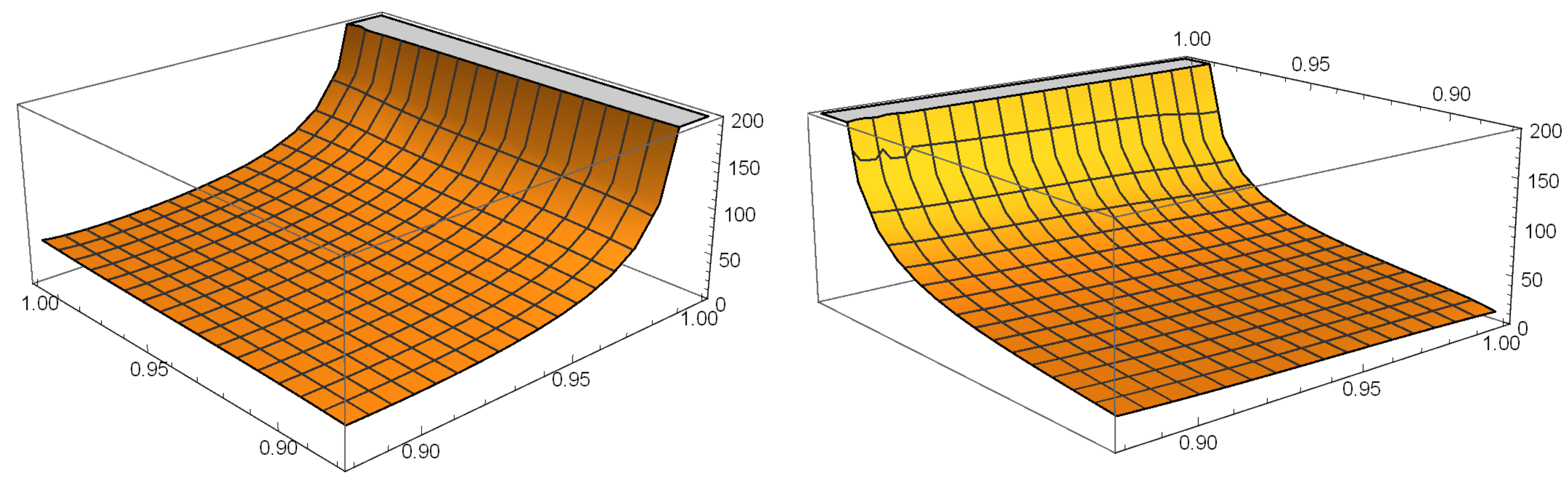
On the contrary, the analysis of the sign of $\partial F_1/\partial k_1$ and $\partial F_{1,2}/\partial k_2$ over the set A is rather involved and we could not perform it exactly. Therefore, we based our argument concerning the existence of the square Q on the numerical evidence given by the plots of their graphs (see Figure 5), for which we used the software Wolfram MATHEMATICA 10.4.1.

References

- Adami, R.; Serra, E.; Tilli, P. Nonlinear dynamics on branched structures and networks. Riv. Mat. Univ. Parma 2017, 8, 109–159. [Google Scholar]
- Cacciapuoti, C.; Finco, D.; Noja, D. Ground state and orbital stability for the NLS equation on a general starlike graph with potentials. Nonlinearity 2017, 30, 3271–3303. [Google Scholar] [CrossRef] [Green Version]
- Noja, D. Nonlinear Schrödinger equation on graphs: recent results and open problems. Philos. Trans. R. Soc. A 2014, 372, 20130002. [Google Scholar] [CrossRef] [PubMed]
- Gnutzmann, S.; Waltner, D. Stationary waves on nonlinear quantum graphs. I. General framework and canonical perturbation theory, Phys. Rev. E 2016, 93, 032204. [Google Scholar] [PubMed]
- Gnutzmann, S.; Waltner, D. Stationary waves on nonlinear quantum graphs. II. Application of canonical perturbation theory in basic graph structures. Phys. Rev. E 2016, 94, 062216. [Google Scholar] [CrossRef] [PubMed]
- Marzuola, J.; Pelinovsky, D.E. Ground states on the dumbbell graph. Appl. Math. Res. Express 2016, 1, 98–145. [Google Scholar] [CrossRef]
- Pelinovsky, D.E.; Schneider, G. Bifurcations of standing localized waves on periodic graphs. Ann. Henri Poincaré 2017, 18, 1185. [Google Scholar] [CrossRef]
- Sobirov, Z.; Matrasulov, D.U.; Sabirov, K.K.; Sawada, S.; Nakamura, K. Integrable nonlinear Schrödinger equation on simple networks: Connection formula at vertices. Phys. Rev. E 2010, 81, 066602. [Google Scholar] [CrossRef] [PubMed] [Green Version]
- Sabirov, K.K.; Sobirov, Z.A.; Babajanov, D.; Matrasulov, D.U. Stationary nonlinear Schrödinger equation on simplest graphs. Phys. Lett. A 2013, 377, 860–865. [Google Scholar] [CrossRef]
- Adami, R.; Cacciapuoti, C.; Finco, D.; Noja, D. Stable standing waves for a NLS on star graphs as local minimizers of the constrained energy. J. Differ. Equ. 2016, 260, 7397–7415. [Google Scholar] [CrossRef] [Green Version]
- Adami, R.; Serra, E.; Tilli, P. NLS ground states on Graphs. Calc. Var. Partial Differ. Equ. 2015, 54, 743–761. [Google Scholar] [CrossRef]
- Adami, R.; Serra, E.; Tilli, P. Threshold phenomena and existence results for NLS ground states on metric graphs. J. Funct. Anal. 2016, 271, 201–223. [Google Scholar] [CrossRef]
- Adami, R.; Serra, E.; Tilli, P. Negative Energy Ground States for the L2-Critical NLSE on Metric Graphs. Comm. Math. Phys. 2017, 352, 387–406. [Google Scholar] [CrossRef]
- Berkolaiko, G.; Kuchment, P. Introduction to Quantum Graphs; Mathematical Surveys and Monographs 186; American Mathematical Society: Providence, RI, USA, 2013. [Google Scholar]
- Noja, D.; Rolando, S.; Secchi, S. Standing waves for the NLS on the double–bridge graph and a rational-irrational dichotomy. J. Differ. Equ. 2019, 451, 147–178. [Google Scholar] [CrossRef]
- Adami, R.; Serra, E.; Tilli, P. Multiple positive bound states for the subcritical NLS equation on metric graphs. Calc. Var. Partial Differ. Equ. 2019, 58. [Google Scholar] [CrossRef]
- Cacciapuoti, C.; Finco, D.; Noja, D. Topology-induced bifurcations for the nonlinear Schrödinger equation on the tadpole graph. Phys. Rev. E 2015, 91, 013206. [Google Scholar] [CrossRef] [PubMed]
- Noja, D.; Pelinovsky, D.; Shaikhova, G. Bifurcation and stability of standing waves in the nonlinear Schrödinger equation on the tadpole graph. Nonlinearity 2015, 28, 2343–2378. [Google Scholar] [CrossRef]
- Lawden, D.F. Elliptic Functions and Applications; Springer: New York, NY, USA, 1989. [Google Scholar]
- Olver, F.W.J.; Lozier, D.W.; Boisvert, R.F.; Clark, C.W. NIST Handbook of Mathematical Functions; Cambridge University Press: New York, NY, USA, 2010. [Google Scholar]
- Niven, I. Diophantine Approximations; Interscience Tracts in Pure and Applied Mathematics No. 14; Interscience Publishers, Wiley & Sons: New York, NY, USA, 1963. [Google Scholar]
Figure 1.
The double-bridge graph.
Figure 2.
Bifurcation diagram for with coprime.
Figure 3.
The appearance of each of the sequences and for .
Figure 4.
The set A. The point and the straight lines of the boundary are not included.
Figure 5.
The functions and over the square with .
© 2019 by the authors. Licensee MDPI, Basel, Switzerland. This article is an open access article distributed under the terms and conditions of the Creative Commons Attribution (CC BY) license (http://creativecommons.org/licenses/by/4.0/).
Share and Cite
MDPI and ACS Style
Noja, D.; Rolando, S.; Secchi, S. A Note on Sign-Changing Solutions to the NLS on the Double-Bridge Graph. Symmetry 2019, 11, 161. https://doi.org/10.3390/sym11020161
AMA Style
Noja D, Rolando S, Secchi S. A Note on Sign-Changing Solutions to the NLS on the Double-Bridge Graph. Symmetry. 2019; 11(2):161. https://doi.org/10.3390/sym11020161
Chicago/Turabian StyleNoja, Diego, Sergio Rolando, and Simone Secchi. 2019. "A Note on Sign-Changing Solutions to the NLS on the Double-Bridge Graph" Symmetry 11, no. 2: 161. https://doi.org/10.3390/sym11020161
Note that from the first issue of 2016, this journal uses article numbers instead of page numbers. See further details here.