Balanced Truncation Model Order Reduction in Limited Frequency and Time Intervals for Discrete-Time Commensurate Fractional-Order Systems

Abstract

In this paper we investigate an implementation of new model order reduction techniques to linear time-invariant discrete-time commensurate fractional-order state space systems to obtain lower dimensional fractional-order models. Since the models of physical systems correctly approximate the physical phenomena of the modeled systems for restricted time and frequency ranges only, a special attention is given to time- and frequency-limited balanced truncation and frequency-weighted methods. Mathematical formulas for calculation of the time- and frequency-limited, as well as frequency-weighted controllability and observability Gramians, are extended to fractional-order systems. An instructive simulation experiment corroborates the potential of the introduced methodology.

1. Introduction

In the field of modeling and simulation of fractional-order systems there are two different approaches to application of model order reduction (MOR) techniques: (1) Approximation of fractional-order systems by high integer-order models and their reduction to the low integer-order ones, and (2) reduction of the fractional-order systems without changing the class of the model, i.e., the reduced model is also the fractional-order one.

The first approach can be implemented by either determination of the fractional-order derivative/difference approximators involved in a fractional-order system [1,2] or by selection of integer-order approximators to the whole fractional-order systems [3,4,5,6,7,8]. In both approaches, a very high integer-order model is usually obtained, which is not effective from the computational point of view due to large memory requirements and long simulation times. For these reasons, classical model reduction techniques can be used to reduce integer-order model dimensions [8,9,10]. Therefore, the term MOR for fractional-order systems is usually related to order reduction of integer-order approximators to fractional-order systems.

This paper tackles the issue of MOR for commensurate fractional-order systems where a final result of using the MOR technique is the fractional-order model of lower dimensions. This issue has not been systematically studied and only a few approaches for reduction of continuous-time fractional-order systems have been published [11,12,13,14].

The classical Balanced Truncation (BT) method introduced for classical integer-order systems has been extended to discrete-time fractional-order systems [15]. The reduction paradigms used by the BT method enforce an accurate approximation for the whole range of frequencies. However, models of physical systems, e.g., models for mechanical, electrical and biological systems, characterize a certain adequacy scope, determined by the frequency range, for which the models correctly approximate the physical phenomena of the modeled systems. Likewise, when the reduced model is used to carry out a simulation in the determined time interval, an appropriate approximation accuracy of the output signal $y(t)$ is required only for t lower than a specified final time of simulation. For these reasons, the reduction aims to determine such a reduced model which is particularly accurate in the given frequency range $[{\omega }_{min},{\omega }_{max}]$ and/or time interval $[t_{min},t_{max}]$. Such an approach allows for larger errors outside these specified intervals, without negative impact on the usefulness of the obtained reduced model. The time and frequency boundaries can be applied either by using frequency- and time-limited controllability and observability Gramians [16,17,18,19] or by frequency-weighted functions connected to the model which are the subject to the reduction process [20,21,22,23,24,25,26]. In this paper, we focus on the generalization of such approaches to reduction and an accurate approximation in given frequency and time intervals for the discrete-time commensurate fractional-order systems.

The remainder of this paper is structured as follows. A description of fractional-order state space systems considered in the paper is introduced in Section 2. Section 3 includes fundamentals of the MOR concept, in particular for the BT method. Section 4 contains the main result of the paper concerning definitions of controllability and observability Gramians in the time- and frequency-domains for fractional-order systems. Numerical examples of Section 5 illustrate the use of the introduced Gramians in the model reduction process. The paper is completed with the conclusion section.

2. System Representation

Consider a linear discrete-time commensurate fractional-order (DTCFO) state space system $G=\{A_f,B,C,D\}$ described by

$$\begin{array}{cc}\hfill {\Delta }^{\alpha }x(k+1)& =A_{f}x(k)+Bu(k),x(0)=x_0\hfill \\ \hfill y(k)& =Cx(k)+Du(k)\hfill \end{array}$$

(1)

where $k=0,1,\cdots$, is the discrete time, $x(k)\in {\Re }^n$ is the state vector, $u(k)$ and $y(k)$ are the input and output signals, respectively. Matrices $A_f\in {\Re }^{n\times n}$, $B\in {\Re }^{n\times n_u}$, $C\in {\Re }^{n_y\times n}$, $D\in {\Re }^{n_y\times n_u}$ describe the system properties, with $n_u$ and $n_y$ being the numbers of inputs and outputs, respectively. ${\Delta }^{\alpha }x(k+1)$ defines the fractional-order difference of order $\alpha \in (0,2)$ which can be represented by the Grünwald-Letnikov fractional difference ([27], ch. 3.5)

$${\Delta }^{\alpha }x(k+1)=\sum _{j=0}^{k+1}{(-1)}^j\left(\genfrac{}{}{0pt}{}{\alpha }{j}\right)x(k-j+1)k=0,1,\cdots$$

(2)

with

$$\left(\genfrac{}{}{0pt}{}{\alpha }{j}\right)=\left\{\begin{array}{cc}1& j=0\hfill \\ \frac{\alpha (\alpha -1)\dots (\alpha -j+1)}{j!}& j>0\hfill \end{array}\right.$$

Assuming the zero initial condition, that is ${\Delta }^{\alpha }x(0)=0$, the $\mathcal{Z}$-transform of the system (1) is given by

$$\begin{array}{cc}\hfill w(z)X(z)& =A_{f}X(z)+BU(z)\hfill \\ \hfill Y(z)& =CX(z)+DU(z)\hfill \end{array}$$

(3)

where $w(z)$ is the $\mathcal{Z}$-transform of the “forward-shifted” fractional-order difference

$$w(z)=z{(1-z^{-1})}^{\alpha }=\sum _{j=0}^{k+1}{(-1)}^j\left(\genfrac{}{}{0pt}{}{\alpha }{j}\right)z^{-j+1}$$

(4)

Remark 1.

The above formulation can be extended to discretized models of continuous time systems. In the case of use of the forward-shifted Euler discretization operator ([27], ch. 3.5) we have

$$s^{\alpha }\approx \frac{1}{h^{\alpha }}w(z)$$

(5)

where $s^{\alpha }$ is the Laplace transform of the fractional-order derivative and h is the sampling period. Discretized models of continuous-time fractional-order systems

$$\begin{array}{cc}\hfill {\Delta }^{\alpha }x(t+h)& =h^{\alpha }{\overline{A}}_{f}x(t)+h^{\alpha }\overline{B}u(t),x(0)=x_0\hfill \\ \hfill y(t)& =Cx(t)+Du(t)\hfill \end{array}$$

(6)

where $t=kh$, can simply be transferred to the system (1) by using the following substitutions

$$A_f\to h^{\alpha }{\overline{A}}_{f}B\to h^{\alpha }\overline{B}$$

(7)

Implementation of the Grünwald–Letnikov difference (2) results in increasing computational burden at each time step, which finally becomes computationally infeasible. Therefore, in practical implementations, finite-length expansions are used, for instance finite fractional difference [6,8] ([28], ch. 7)

$${\Delta }^{\alpha }x(k+1)\approx \sum _{j=0}^L{(-1)}^j\left(\genfrac{}{}{0pt}{}{\alpha }{j}\right)x(k-j+1)k=0,1,\cdots$$

(8)

with $x(l)=0\forall l<0$ and L being the implementation length.

It is worth emphasizing that precise approximation of the Grünwald–Letnikov difference with the finite fractional difference needs a very high length L [6].

3. Model Order Reduction

Let us shift now to the MOR problem for the DTCFO system (1). The fractional-order MOR issue aims towards finding a DTCFO model $\tilde{G}$ with reduced dimension $r<n$

$$\begin{array}{cc}\hfill {\Delta }^{\alpha }\tilde{x}(k+1)& ={\tilde{A}}_f\tilde{x}(k)+\tilde{B}u(k),\tilde{x}(0)={\tilde{x}}_0\hfill \\ \hfill \tilde{y}(k)& =\tilde{C}\tilde{x}(k)+\tilde{D}u(k)\hfill \end{array}$$

(9)

where ${\tilde{A}}_f\in {\Re }^{r\times r}$, $\tilde{B}\in {\Re }^{r\times n_u}$, $\tilde{C}\in {\Re }^{n_y\times r}$, $\tilde{D}\in {\Re }^{n_y\times n_u}$, $\tilde{x}(k)\in {\Re }^r$ are such that the approximation errors both in the time domain $\parallel y(k)-\tilde{y}(k)\parallel$ and in the frequency domain $\parallel G(z)-\tilde{G}(z)\parallel$ are small for the chosen norm $\parallel ·\parallel$.

In this paper, we concentrate on the BT technique, which is based on the concept of the balanced model realization [29,30], ([31], ch. 7.1). In order to arrive at the balanced system, the linear state transformation $x\to Tx$ is applied to diagonalize the controllability P and observability Q Gramians of the system

$$TP{T}^T={(T^T)}^{-1}Q{T}^{-1}=\mathrm{diag}\left({\sigma }_1,\dots ,{\sigma }_n\right)$$

(10)

where ${\sigma }_i$, $i=1,\dots ,n$, are the square roots of the eigenvalues for the product of P and Q, which are called the Hankel singular values (HSV). The magnitude of HSV classifies a degree of reachability and observability of states in the system. On this basis, reduction eliminates states corresponding to small values ${\sigma }_i$, which means that they have a weak impact on the system properties. The balanced model is obtained by applying transformation matrices in the following way:

$$T{A}_f{T}^{-1}=\left[\begin{array}{cc}{\tilde{A}}_f& {\tilde{A}}_{12}\\ {\tilde{A}}_{21}& {\tilde{A}}_{22}\end{array}\right],TB=\left[\begin{array}{c}\tilde{B}\\ {\tilde{B}}_2\end{array}\right],C{T}^{-1}=\left[\begin{array}{cc}\tilde{C}& {\tilde{C}}_2\end{array}\right],\tilde{D}=D$$

(11)

The order r can be selected on the basis of an approximation error of the reduced system. For the BT method, the ${\mathcal{H}}_{\infty }$ norm of the approximation error is upper bounded as follows [30], ([31], ch. 7.2):

$${∥G(z)-\tilde{G}(z)∥}_{{\mathcal{H}}_{\infty }}\le 2\sum _{j=r+1}^n{\sigma }_j$$

(12)

Calculation of the transformation matrix T is not a unique operation. The exemplary algorithms can be found in References [23,30] ([31], ch. 7.3), [32].

The BT reduction method enforces an accurate approximation for all times $t\in (0,\infty )$ and frequencies $\omega \in \Re$. If it is necessary to determine a model (9) which is particularly accurate in a given frequency range $[{\omega }_{min},{\omega }_{max}]$ and/or time interval $[k_{min},k_{max}]$, then frequency- or time-limited controllability and observability Gramians can be used to calculate the transformation matrix T instead of infinite ones. Higher model accuracy can be obtained now, especially when the optimal values of the parameters of the weighting functions and frequency-/time-intervals are used [33].

4. Controllability and Observability Gramians for Discrete-Time Fractional-Order Systems

In this section, the definitions of controllability and observability Gramians both in the time- and frequency-domains are recalled. Based on the definitions for integer-order systems, the Gramian generalizations to fractional-order systems are derived here.

4.1. Gramians in the Time Domain

The definition of the controllability Gramian is connected to the minimal energy required for the transfer of the system from the zero initial state $x(0)=0$ to the final state $x(k)=x_p$, whereas the observability Gramian is defined with relation to the energy generated by the nonzero initial state $x(0)=x_0$ with the zero input signal $u(k)=0$. For asymptotically stable systems, the infinite controllability and observability Gramians are respectively defined as

$$P=\sum _{k=0}^{\infty }\xi (k){\xi }^T(k),Q=\sum _{k=0}^{\infty }{\eta }^T(k)\eta (k)$$

(13)

where $\xi (k)$ is the state of the discrete-time system resulting from the input in the form of the Kronecker delta, and $\eta (k)$ is the output of the system produced by the nonzero initial conditions and the zero input signal.

For asymptotically stable integer-order systems, we obtain the well-known formulas for the controllability and observability Gramians, respectively:

$$P=\sum _{i=0}^{\infty }{A}^{i}B{B}^T{\left(A^T\right)}^i,Q=\sum _{i=0}^{\infty }{\left(A^T\right)}^i{C}^{T}C{A}^i$$

(14)

where $A=A_f+I$. Finally, the Gramians P and Q are the solutions to the discrete-time Lyapunov equations, respectively, are

$$AP{A}^T-P=-B{B}^T,A^{T}QA-Q=-C^{T}C.$$

(15)

Based on definitions (13), it is easy to formulate the generalized form of the controllability and observability Gramians for the fractional-order systems.

Lemma 1.

Consider an asymptotically stable discrete-time commensurate fractional-order state space system (1), with the Grünwald–Letnikov fractional-order difference (2). Then the controllability and observability Gramians at finite time $k_L<\infty$ are as follows

$$P(k_L)=\sum _{k=1}^{k_L}\varphi (k-1)B{B}^T{\varphi }^T(k-1),Q(k_L)=\sum _{k=0}^{k_L}{\varphi }^T(k)C^{T}C\varphi (k)$$

(16)

where $\varphi (k)$, $k=0,1,\dots$, are calculated as

$$\varphi (k)=\left\{\begin{array}{cc}I& k=0\hfill \\ (A_f+\alpha I)\varphi (k-1)-{\displaystyle \sum _{j=2}^k}{(-1)}^j\left(\genfrac{}{}{0pt}{}{\alpha }{j}\right)\varphi (k-j)& k>0\hfill \end{array}\right.$$

Proof. 

The state space equations of the system as in Equation (1) can be rewritten as ([27], ch. 3.5)

$$\begin{array}{cc}\hfill x(k+1)& =(A_f+\alpha I)x(k)-\sum _{i=2}^{k+1}{(-1)}^i\left(\genfrac{}{}{0pt}{}{\alpha }{i}\right)x(k+1-i)+Bu(k)\hfill \\ \hfill y(k)& =Cx(k)+Du(k)\hfill \end{array}$$

(17)

The state response for the DTCFO system (17), with the zero initial condition and the Kronecker delta input signal, is as follows:

$$\xi (k)=\left\{\begin{array}{cc}0& k=0\hfill \\ B& k=1\hfill \\ (A_f+\alpha I)\xi (k-1)-{\displaystyle \sum _{j=2}^k}{(-1)}^j\left(\genfrac{}{}{0pt}{}{\alpha }{j}\right)\xi (k-j)& k>1\hfill \end{array}\right.$$

(18)

The output response for the DTCFO system (17), with the nonzero initial condition $x(0)=x_0$ and the zero input signal, is now

$$y(k)=\eta (k)x(0)$$

(19)

where

$$\eta (k)=\left\{\begin{array}{cc}C& k=0\hfill \\ C\left((A_f+\alpha I)x(k-1)-{\displaystyle \sum _{j=2}^k}{(-1)}^j\left(\genfrac{}{}{0pt}{}{\alpha }{j}\right)x(k-j))\right)& k>0\hfill \end{array}\right.$$

(20)

The responses (18) and (20) immediately result in Equation (16), which completes the proof.  □

Remark 2.

As mentioned before, both the minimal energy required for the transfer of the system from the zero initial state to $x(k)=x_p$ and the energy generated by the nonzero initial state are obtained for $k_L\to \infty$. Implementation of Equation (16) in order to calculate controllability and observability Gramians implies the infinite number of elements $\varphi (k)$. Furthermore each of $\varphi (k)$ requires the determination of the Grünwald–Letnikov difference calculated from 0 to $k+1$, which is computationally infeasible. Therefore, in contrast to integer-order systems for which the solution of Equation (13) can be determined by solving Lyapunov Equation (15), the Gramians for the fractional-order systems can be calculated for the finite length only.

If the response of the reduced model (9) is expected to match the original fractional-order model (1) in some interval $[k_1,k_2]$, then the balancing of the model can be executed on the basis of the Gramians calculated within this restricted time interval. As the controllability and observability Gramians for the asymptotically stable systems are positive definite, then it can be shown that

$$P(k_2)\ge P(k_1)Q(k_2)\ge Q(k_1)\mathrm{for}{k}_2\ge k_1$$

(21)

Therefore, the time-limited Gramians are also positive definite, and within the restricted time interval $[k_1,k_2]$ they can be calculated as follows:

$$P(k_1,k_2)=P(k_2)-P(k_1),Q(k_1,k_2)=Q(k_2)-Q(k_1)$$

(22)

where $P(k)$ and $Q(k)$ are given from Equation (16).

4.2. Gramians in the Frequency Domain

In addition to the definition (13) given in the time domain, the Gramians can also be expressed in the frequency domain. The connection can be made on the basis of the Plancherel’s theorem, which states that the integral of the inner product of two functions in the time domain is equal to the integral of their frequency spectrum. In particular, for the asymptotically stable discrete-time integer-order systems, applying the Plancherel’s theorem to Equation (14) yields ([31], ch. 4.3)

$$\begin{array}{cc}\hfill P& =\frac{1}{2\pi }{\int }_0^{2\pi }{\left(e^{j\theta }I-A\right)}^{-1}B{B}^T{\left((e^{-j\theta }I-A^T\right)}^{-1}d\theta \hfill \\ \hfill Q& =\frac{1}{2\pi }{\int }_0^{2\pi }{\left(e^{-j\theta }I-A^T\right)}^{-1}{C}^{T}C{\left(e^{j\theta }I-A\right)}^{-1}d\theta \hfill \end{array}$$

(23)

Based on definitions (23), it is easy to formulate the generalized form of the controllability and observability Gramians for the fractional-order systems.

Lemma 2.

Consider an asymptotically stable discrete-time commensurate fractional-order state space system (1), with the Grünwald–Letnikov fractional-order difference (2). Then the infinite controllability and observability Gramians of the fractional-order system are respectively given as

$$\begin{array}{c}\hfill P=\frac{1}{2\pi }{\int }_{-\pi }^{+\pi }{\left(w(z)I-A_f\right)}^{-1}B{B}^T{\left(w^{\ast }(z)I-A_f^T\right)}^{-1}d\theta \\ \hfill Q=\frac{1}{2\pi }{\int }_{-\pi }^{+\pi }{\left(w^{\ast }(z)I-A_f^T\right)}^{-1}{C}^{T}C{\left(w(z)I-A_f\right)}^{-1}d\theta \end{array}$$

(24)

where $w(z)$ is as in Equation (4), with $z=e^{i\theta }$, $\theta \in [-\pi ,\pi ]$, and * denotes the complex conjugate transpose.

Proof. 

For continuous-time fractional-order systems referred to in Remark 1, the input-to-state map becomes ${(s^{\alpha }I-{\overline{A}}_f)}^{-1}\overline{B}$, while the state-to-output map is $C{(s^{\alpha }I-{\overline{A}}_f)}^{-1}$. Then the controllability and observability Gramians are as follows:

$$\begin{array}{c}\hfill P=\frac{1}{2\pi }{\int }_{-\infty }^{\infty }{\left(s^{\alpha }I-{\overline{A}}_f\right)}^{-1}\overline{B}{\overline{B}}^T{\left({(s^{\alpha })}^{\ast }I-{\overline{A}}_f^T\right)}^{-1}d\omega \\ \hfill Q=\frac{1}{2\pi }{\int }_{-\infty }^{\infty }{\left({(s^{\alpha })}^{\ast }I-{\overline{A}}_f^T\right)}^{-1}{C}^{T}C{\left(s^{\alpha }I-{\overline{A}}_f\right)}^{-1}d\omega \end{array}$$

(25)

where $s=i\omega$, $\omega \in (-\infty ,\infty )$. Using the forward-shifted Euler discretization operator as referred to in Remark 1 results immediately in (24), which completes the proof.  □

If the response of the reduced model is expected to match the full fractional-order model output within a restricted frequency range, then the balancing of the model can be executed on the basis of the Gramians calculated for that specific interval. Similarly, as for time-limited Gramians, the frequency-limited Gramians in restricted frequency interval $[{\Theta }_1,{\Theta }_2]$ can be calculated as follows:

$$P({\Theta }_1,{\Theta }_2)=P({\Theta }_2)-P({\Theta }_1),Q({\Theta }_1,{\Theta }_2)=Q({\Theta }_2)-Q({\Theta }_1)$$

(26)

where $P(\Theta )$ and $Q(\Theta )$ are given as

$$\begin{array}{c}\hfill P(\Theta )=\frac{1}{2\pi }{\int }_{-\Theta }^{+\Theta }{\left(w(z)I-A_f\right)}^{-1}B{B}^T{\left(w^{\ast }(z)I-A_f^T\right)}^{-1}d\theta \\ \hfill Q(\Theta )=\frac{1}{2\pi }{\int }_{-\Theta }^{+\Theta }{\left(w^{\ast }(z)I-A_f^T\right)}^{-1}{C}^{T}C{\left(w(z)I-A_f\right)}^{-1}d\theta \end{array}$$

(27)

4.3. Frequency Weighted Gramians

The required approximation accuracy in the given frequency interval $[{\Theta }_1,{\Theta }_2]$ can also be achieved by implementation of the frequency weighting functions in a form of the external systems connected to the inputs and/or outputs of the full fractional-order model ([31], ch. 7.6). Such an approach, called Frequency Weighted (FW) method, is a generalization to the BT method designed for asymptotically stable models with asymptotically stable input and output weighting functions with minimal realizations.

Consider an asymptotically stable discrete-time integer- or fractional-order LTI MIMO state space system as an input weighting function $H_i=\{A_i,B_i,C_i,D_i\}$

$$\begin{array}{cc}\hfill {\Delta }^{{\alpha }_i}{x}_i(k+1)& =A_i{x}_i(k)+B_i{u}_i(k),\hfill \\ \hfill y_i(k)& =C_i{x}_i(k)+D_i{u}_i(k)\hfill \end{array}$$

(28)

and as an output weighting function $H_o=\{A_o,B_o,C_o,D_o\}$

$$\begin{array}{cc}\hfill {\Delta }^{{\alpha }_o}{x}_o(k+1)& =A_o{x}_o(k)+B_o{u}_o(k),\hfill \\ \hfill y_o(k)& =C_o{x}_o(k)+D_o{u}_o(k)\hfill \end{array}$$

(29)

of orders $n_i$ and $n_o$, respectively. Assuming that no pole-zero cancellations occur during the design of the augmented systems $G{H}_i$ and $H_{o}G$, we arrive at [22,25], ([31], ch. 7.6)

$$\begin{array}{c}\hfill G{H}_i& =\left[\begin{array}{cc}{\tilde{A}}_i& {\tilde{B}}_i\\ {\tilde{C}}_i& {\tilde{D}}_i\end{array}\right]=\left[\begin{array}{ccc}{A}_f& B{C}_i& B{D}_i\\ 0& A_i& B_i\\ C& D{C}_i& D{D}_i\end{array}\right]\hfill \\ \hfill H_{o}G& =\left[\begin{array}{cc}{\tilde{A}}_o& {\tilde{B}}_o\\ {\tilde{C}}_o& {\tilde{D}}_o\end{array}\right]=\left[\begin{array}{ccc}{A}_f& 0& B\\ B_{o}C& A_o& B_{o}D\\ D_{o}C& C_o& D_{o}D\end{array}\right]\hfill \end{array}$$

(30)

It is well known that the frequency weighted controllability and observability Gramians are computed on the basis of the system connected to the input weight $G{H}_i$ and to the output weight $H_{o}G$, respectively.

Lemma 3.

Consider asymptotically stable augmented systems $G{H}_i$ and $H_{o}G$ as in Equation (30) consisting of asymptotically stable discrete-time commensurate fractional-order state space system (1), with the Grünwald–Letnikov fractional-order difference (2) and the weighting functions as in Equations (28) and (29). The controllability and observability Gramians of such systems at finite time $k_L<\infty$ are as follows:

$$P_i(k_L)=\sum _{k=1}^{k_L}{\varphi }_i(k-1){\tilde{B}}_i{\tilde{B}}_i^T{\varphi }_i^T(k-1),Q_o(k_L)=\sum _{k=0}^{k_L}{\varphi }_o^T(k){\tilde{C}}_o^T{\tilde{C}}_o{\varphi }_o(k)$$

(31)

where ${\varphi }_i(k)$, ${\varphi }_o(k)$, $k=0,1,\dots$, are calculated in a recurrent way:

$$\begin{array}{c}\hfill {\varphi }_i(k)=\left\{\begin{array}{cc}I& k=0\hfill \\ \left({\tilde{A}}_i+{\tilde{\alpha }}_i\right){\varphi }_i(k-1)-\sum _{j=2}^k{\psi }_i(j){\varphi }_i(k-j)& k>0\hfill \end{array}\right.\\ \hfill {\varphi }_o(k)=\left\{\begin{array}{cc}I& k=0\hfill \\ \left({\tilde{A}}_o+{\tilde{\alpha }}_o\right){\varphi }_o(k-1)-\sum _{j=2}^k{\psi }_o(j){\varphi }_o(k-j)& k>0\hfill \end{array}\right.\end{array}$$

with ${\tilde{\alpha }}_i=diag(\underset{n}{\underbrace{\alpha ,\cdots ,\alpha }},\underset{n_i}{\underbrace{{\alpha }_i,\cdots ,{\alpha }_i}})$, ${\tilde{\alpha }}_o=diag(\underset{n}{\underbrace{\alpha ,\cdots ,\alpha }},\underset{n_o}{\underbrace{{\alpha }_o,\cdots ,{\alpha }_o}})$ and

$$\begin{array}{c}\hfill {\psi }_i(j)={(-1)}^{j}diag\left(\underset{n}{\underbrace{\left(\genfrac{}{}{0pt}{}{\alpha }{j}\right),\cdots ,\left(\genfrac{}{}{0pt}{}{\alpha }{j}\right)}},\underset{n_i}{\underbrace{\left(\genfrac{}{}{0pt}{}{{\alpha }_i}{j}\right),\cdots ,\left(\genfrac{}{}{0pt}{}{{\alpha }_i}{j}\right)}}\right)\\ \hfill {\psi }_o(j)={(-1)}^{j}diag\left(\underset{n}{\underbrace{\left(\genfrac{}{}{0pt}{}{\alpha }{j}\right),\cdots ,\left(\genfrac{}{}{0pt}{}{\alpha }{j}\right)}},\underset{n_o}{\underbrace{\left(\genfrac{}{}{0pt}{}{{\alpha }_o}{j}\right),\cdots ,\left(\genfrac{}{}{0pt}{}{{\alpha }_o}{j}\right)}}\right)\end{array}$$

Proof. 

The proof directly stems from proof for Lemma 1 with substitution of the system matrices by the matrices of the augmented systems $G{H}_i$ and $H_{o}G$.  □

Note that the application of the weighting functions influences the order of the controllability $P_i$ and observability $Q_o$ Gramians for the augmented systems. Therefore, they are partitioned into two-by-two blocks, so that the dimension of the $P_{11}\in {\Re }^{n\times n}$ and $Q_{11}\in {\Re }^{n\times n}$ are the same as the state matrix $A_f$

$$P_i=\left[\begin{array}{cc}{P}_{11}& P_{12}\\ P_{12}^T& P_{22}\end{array}\right],Q_o=\left[\begin{array}{cc}{Q}_{11}& Q_{12}\\ Q_{12}^T& Q_{22}\end{array}\right]$$

(32)

Finally, the frequency-weighted controllability $\tilde{P}$ and observability $\tilde{Q}$ Gramians of dimensions $n\times n$ can be assumed as [20]

$$\tilde{P}=P_{11},\tilde{Q}=Q_{11}$$

(33)

The proposed solution, despite its simplicity, may lead to the instability of the reduced model in case of two-sided weighting. Therefore, several modifications to this approach have been proposed to cope with this problem [21,22,23,24,25].

The frequency-weighted Gramians as in Equation (33) can also be defined in the frequency domain. Given that the input-to-state map and the state-to-output map of the fractional-order system are modified by the connected weighting functions, it is possible to generalize the definitions of the infinite controllability and observability Gramians for the fractional-order system (Lemma 2) to the frequency-weighted Gramians.

Lemma 4.

Consider asymptotically stable augmented systems $G{H}_i$ and $H_{o}G$ as in Equation (30), consisting of asymptotically stable discrete-time commensurate fractional-order state space system (1), with the Grünwald–Letnikov fractional-order difference (2) and the weighting functions as in Equations (28) and (29). Then the frequency-weighted controllability $\tilde{P}$ and observability $\tilde{Q}$ Gramians are defined as

$$\begin{array}{cc}\hfill \tilde{P}& =\frac{1}{2\pi }{\int }_{-\pi }^{\pi }{\left(w(z)I-A_f\right)}^{-1}B{H}_i\left(w_i(z)\right)H_i^T\left(w_i^{\ast }(z)\right)B^T{\left(w^{\ast }(z)I-A_f^T\right)}^{-1}d\theta \hfill \\ \hfill \tilde{Q}& =\frac{1}{2\pi }{\int }_{-\pi }^{\pi }{\left(w^{\ast }(z)I-A_f^T\right)}^{-1}{C}^T{H}_o^T\left(w_o^{\ast }(z)\right)H_o\left(w_o(z)\right)C{\left(w(z)I-A_f\right)}^{-1}d\theta \hfill \end{array}$$

(34)

where $H_i\left(w_i(z)\right)=D_i+C_i{(w_i(z)I-A_i)}^{-1}{B}_i$, $H_o\left(w_o(z)\right)=D_o+C_o{(w_o(z)I-A_o)}^{-1}{B}_o$ and$w(z)=z{(1-z^{-1})}^{\alpha }$, $w_i(z)=z{(1-z^{-1})}^{{\alpha }_i}$, $w_o(z)=z{(1-z^{-1})}^{{\alpha }_o}$, with $z=e^{i\theta }$, $\theta \in [-\pi ,\pi ]$.

Proof. 

Given that the input-to-state map for the augmented system $G{H}_i$ and the state-to-output map for $H_{o}G$ become ${\left({\tilde{w}}_i(z)-{\tilde{A}}_i\right)}^{-1}{\tilde{B}}_i$ and ${\tilde{C}}_o{\left({\tilde{w}}_o(z)-{\tilde{A}}_o\right)}^{-1}$, where ${\tilde{w}}_i(z)=\mathrm{diag}\left(\underset{n}{\underbrace{w(z),\cdots ,w(z)}},\underset{n_i}{\underbrace{w_i(z),\cdots ,w_i(z)}}\right)$ and ${\tilde{w}}_o(z)=\mathrm{diag}\left(\underset{n}{\underbrace{w(z),\cdots ,w(z)}},\underset{n_o}{\underbrace{w_o(z),\cdots ,w_o(z)}}\right)$, respectively. The $\tilde{P}$ and $\tilde{Q}$ are the submatrices of the Gramians for the augmented systems (32) partitioned into two-by-two blocks. Therefore, the proof for the frequency-weighted controllability Gramian follows by noticing that

$$\begin{array}{c}\left(\begin{array}{cc}I& 0\end{array}\right){\left(\left[\begin{array}{cc}w(z)I& 0\\ 0& w_i(z)I\end{array}\right]-\left[\begin{array}{cc}{A}_f& B{C}_i\\ 0& A_i\end{array}\right]\right)}^{-1}\left[\begin{array}{c}B{D}_i\\ B_i\end{array}\right]=\hfill \\ \left(\begin{array}{cc}I& 0\end{array}\right){\left[\begin{array}{cc}w(z)I-A_f& -B{C}_i\\ 0& w_i(z)I-A_i\end{array}\right]}^{-1}\left[\begin{array}{c}B{D}_i\\ B_i\end{array}\right]=\hfill \\ \left(\begin{array}{cc}I& 0\end{array}\right)\left[\begin{array}{cc}{(w(z)I-A_f)}^{-1}& {(w(z)I-A_f)}^{-1}B{C}_i{(w_i(z)I-A_i)}^{-1}\\ 0& {(w_i(z)I-A_i)}^{-1}\end{array}\right]\left[\begin{array}{c}B{D}_i\\ B_i\end{array}\right]=\hfill \\ {(w(z)I-A_f)}^{-1}B(D_i+C_i{(w_i(z)I-A_i)}^{-1}{B}_i)={(w(z)I-A_f)}^{-1}B{H}_i(w_i(z))\hfill \end{array}$$

while for the frequency-weighted observability Gramian,

$$\begin{array}{c}\left[\begin{array}{cc}{D}_{o}C& C_o\end{array}\right]{\left(\left[\begin{array}{cc}w(z)I& 0\\ 0& w_o(z)I\end{array}\right]-\left[\begin{array}{cc}{A}_f& 0\\ B_{o}C& A_o\end{array}\right]\right)}^{-1}\left(\begin{array}{c}I\\ 0\end{array}\right)=\hfill \\ \left[\begin{array}{cc}{D}_{o}C& C_o\end{array}\right]{\left[\begin{array}{cc}w(z)I-A_f& 0\\ -B_{o}C& w_o(z)I-A_o\end{array}\right]}^{-1}\left(\begin{array}{c}I\\ 0\end{array}\right)=\hfill \\ \left[\begin{array}{cc}{D}_{o}C& C_o\end{array}\right]\left[\begin{array}{cc}{(w(z)I-A_f)}^{-1}& 0\\ {(w_o(z)I-A_o)}^{-1}{B}_{o}C{(w(z)I-A_f)}^{-1}& {(w_o(z)I-A_o)}^{-1}\end{array}\right]\left(\begin{array}{c}I\\ 0\end{array}\right)=\hfill \\ (D_o+C_o{(w_o(z)I-A_o)}^{-1}{B}_o){(w(z)I-A_f)}^{-1}B=H_o(w_o(z)){(w(z)I-A_f)}^{-1}B\hfill \end{array}$$

Therefore, the frequency-weighted Gramians are the blocks $P_{11}$ and $Q_{11}$ of the controllability $P_i$ and observability $Q_o$ Gramians for the augmented systems, respectively, which completes the proof.  □

Remark 3.

It is important to note that Lemmas 1 to 4 introduce various definitions of controllability and observability Gramians. However, the calculations of the Gramians directly from the above definitions for large-scale DTCFO systems are computationally demanding. In particular, time-domain Gramian definitions as in Lemma 1 and 3 are infeasible for large-scale systems due to the requirement of calculation of the Grünwald–Letnikov difference from 0 to $k+1$. The common practice for integer order systems when $n_u,n_y<<n$ is to compute low-rank approximations of the Gramians such that $P\approx SY{S}^T$ with $S\in {\Re }^{n\times l}$, $Y\in {\Re }^{l\times l}$, $l<<n$. It is motivated by the typical rapid decay of HSV [34,35], which can also be assumed for fractional-order systems. There exists various algorithms for calculating the low-rank Gramian factorizations for integer-order systems [17,19,35,36]. Therefore, future works will be carried out towards the extension of the low-rank approach to increase the efficiency of Gramians calculations for DTCFO systems.

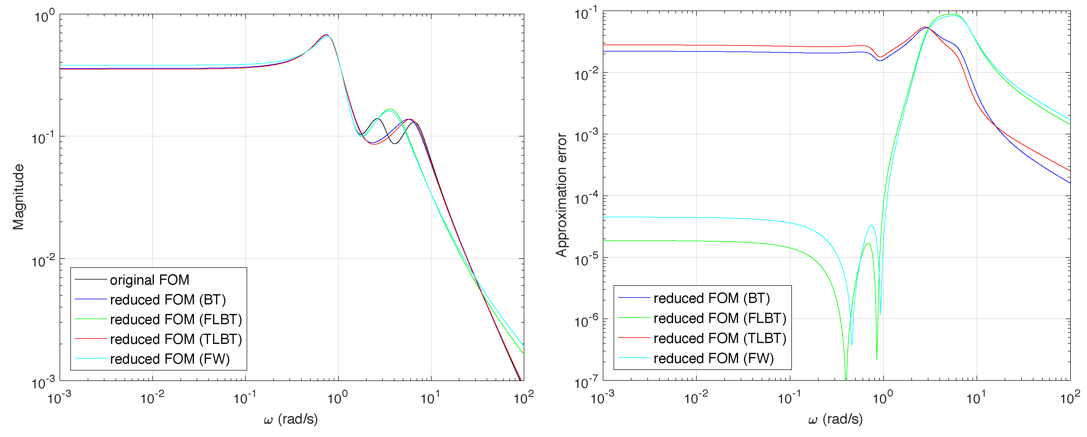
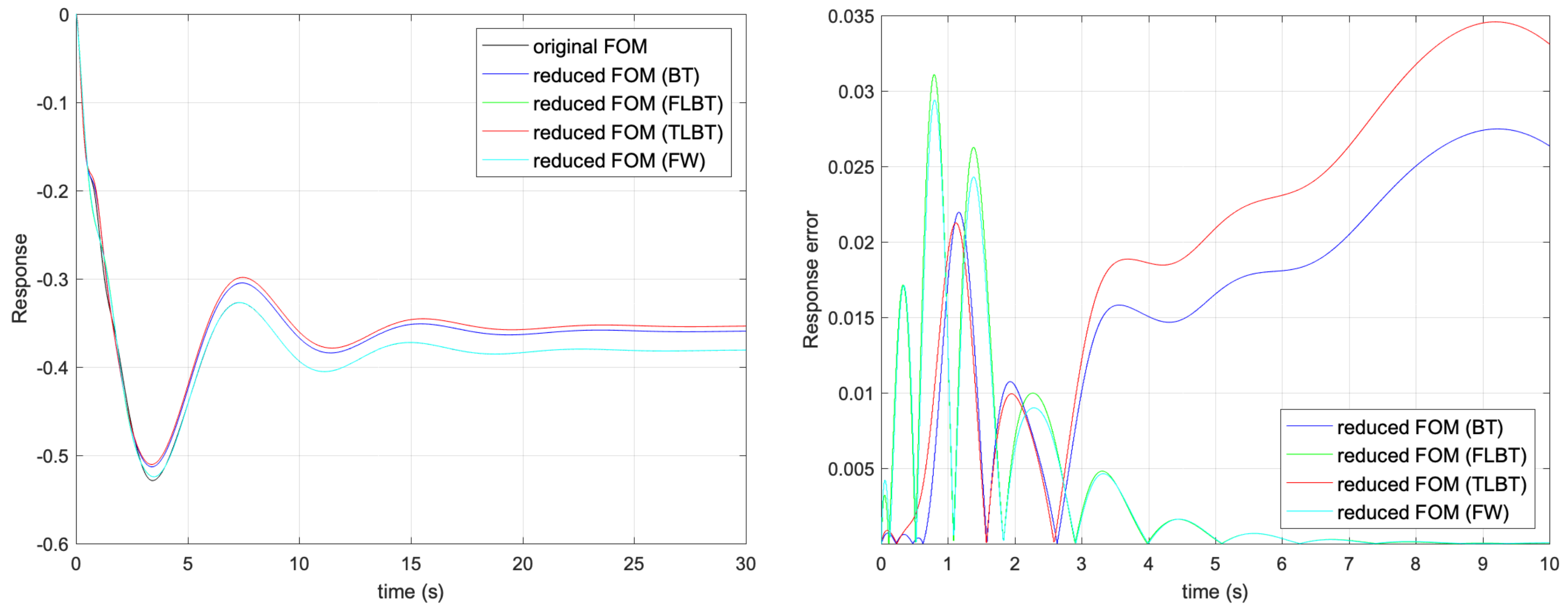
5. Simulation Examples

In this section, examples of model order reduction for a fractional-order system are presented. All reduced models were obtained by using the BT method with the Gramians calculated within various time- and frequency-intervals, as well as with different frequency-weighted functions. In particular, to calculate transformation matrix T the following Gramians are selected: (1) indefinite Gramians defined in the frequency domain as in Equation (24) - denoted as the BT, (2) frequency-limited Gramians as in Equation (26), denoted as the FLBT, (3) time-limited Gramians as in Equation (16), denoted as the TLBT, (4) frequency-weighted Gramians as in Equation (34), denoted as the FW. The examined discrete-time fractional-order model is an extension of the continuous-time model for a simple mechanical system presented in [16] and (moderate) large-scale dynamical system of order 1006 as in [36].

Example 1.

Consider the DTCFO state space system (6) with the sampling period $h=0.01$, fractional order $\alpha =0.85$ and

$$\left[\begin{array}{cc}{\overline{A}}_f& \overline{B}\\ C& D\end{array}\right]=\left[\begin{array}{ccccccc}0& 0& 0& 1& 0& 0& 0\\ 0& 0& 0& 0& 1& 0& 0\\ 0& 0& 0& 0& 0& 1& 0\\ -5.4545& 4.5455& 0& -0.0545& 0.0455& 0& 0.0909\\ 10& -21& 11& 0.1& -0.21& 0.11& 0.4\\ 0& 5.5& -6.5& 0& 0.055& -0.065& -0.5\\ 2& -2& 3& 0& 0& 0& 0\end{array}\right]$$

Model order reduction is performed from the original six states variables to the reduced four ones. Frequency responses for the full fractional-order system and the reduced models in addition to approximation errors are depicted in Figure 1. Figure 2 shows step responses and their approximation errors for the same models. It is clearly visible that the reduction based on infinite and time-limited Gramians for the time interval $t\in \left[0,10\right]$ (s) cannot properly approximate the low-frequency properties of the system. For this reason, in order to improve the approximation for low frequencies, the frequency-interval for frequency-limited Gramians is chosen as $\Theta \in [0,0.01]$ (rad/s). For the same purpose, the low-pass Butterworth filter of order $n_f=5$ and cut-off frequency ${\omega }_f=0.01$ (rad/s) is selected as a frequency weighted function.

Table 1. Frequency and step approximation errors for the reduced models.

	$\mathbf{DCE}$	${\mathit{MSE}}_{\mathit{\omega }}$	${\mathcal{H}}_{\mathbf{\infty }}$	${\mathit{MSE}}_{\mathit{t}}$
BT	$22.2\times {10}^{-3}$	$4.58\times {10}^{-4}$	$53.0\times {10}^{-3}$	$4.62\times {10}^{-4}$
FLBT	$1.88\times {10}^{-5}$	$2.68\times {10}^{-10}$	$88.8\times {10}^{-3}$	$6.37\times {10}^{-6}$
TLBT	$28.1\times {10}^{-3}$	$7.33\times {10}^{-4}$	$54.9\times {10}^{-3}$	$7.40\times {10}^{-4}$
FW	$4.52\times {10}^{-5}$	$1.42\times {10}^{-9}$	$83.7\times {10}^{-3}$	$5.60\times {10}^{-6}$

presents approximation errors for the considered models, where $DCE$ is the steady state approximation error, $MS{E}_{\omega }$ is the mean square approximation error for the frequency responses in the frequency range $\omega \in [{10}^{-3},1]$ (rad/s), ${\mathcal{H}}_{\infty }$ is the norm approximation error and $MS{E}_t$ is the mean square error for system step response in the discrete-time range $t\in [0,100]$ (s).

Figure 3 presents frequency responses and approximation errors for the reduced models obtained in order to improve the quality of approximation for high frequencies. In particular, the third resonance frequency $\omega =6.5$ (rad/s) is considered. Figure 4 shows the impulse responses and their approximation errors for the same models. For this purpose, the time interval $t\in [0,0.1]$ (s) and frequency interval $\Theta \in [0.1,100\pi ]$ (rad/s) are selected for time- and frequency-limited Gramians. Similarly, the frequency weighted function is chosen in a form of a high-pass Butterworth filter of order $n_f=5$ and cut-off frequency ${\omega }_f=0.1$ (rad/s).

Table 2. Frequency and impulse approximation errors for the reduced models.

	${\mathit{MSE}}_{\mathit{\omega }}$	${\mathcal{H}}_{\mathbf{\infty }}$	${\mathit{MSE}}_{\mathit{t}}$
BT	$2.54\times {10}^{-4}$	$0.053$	$9.21\times {10}^{-8}$
FLBT	$3.46\times {10}^{-5}$	$0.538$	$3.23\times {10}^{-8}$
TLBT	$3.68\times {10}^{-5}$	$0.385$	$5.05\times {10}^{-14}$
FW	$4.31\times {10}^{-5}$	$0.539$	$2.24\times {10}^{-8}$

presents approximation errors for the analyzed models, in terms of $MS{E}_{\omega }$ for $\omega >3$ (rad/s), ${\mathcal{H}}_{\infty }$-norm and $MS{E}_t$ for system impulse responses within $t\in [0,1]$ (s).

Example 2.

Consider the system as in reference [36] with fractional-order $\alpha =0.95$ which is discretized using the sampling period $h=0.002$. The calculation of controllability and observability Gramians in the time domain is very computationally demanding for systems of order $n=1006$. Therefore, the reduced models obtained by using only the BT, FLBT and FW methods are compared. All reduced models are of order $r=6$. Frequency responses for the full fractional-order system and the reduced models as well as approximation errors are presented in Figure 5. Like in Example 1, it is clearly visible that the reduction based on the infinite Gramians cannot properly approximate the low-frequency properties of the system. For this reason, the frequency-interval for frequency-limited Gramians and frequency weighting functions are chosen the same as in Example 1. In

Table 3. Frequency and step approximation errors for the reduced models.

	$\mathit{DCE}$	${\mathit{MSE}}_{\mathit{\omega }}$	${\mathcal{H}}_{\mathbf{\infty }}$
BT	$5.538$	$29.93$	$5.538$
FLBT	$4.94\times {10}^{-4}$	$1.90\times {10}^{-7}$	$11.12$
FW	$6.30\times {10}^{-4}$	$3.14\times {10}^{-7}$	$11.35$

, approximation errors are listed for the analyzed models, in terms of $DCE$, $MS{E}_{\omega }$ and ${\mathcal{H}}_{\infty }$-norm.

The Matlab scripts used to compute the presented results can be obtained from Supplementary Materials.

6. Conclusions

This paper presents new results in BT model order reduction in limited time- and frequency- intervals for DTCFO systems. The main contribution of the paper is an introduction of new definitions for controllability and observability Gramians for the fractional-order systems both in the time and frequency domains. These results enable new implementations of the Gramians in the balanced truncation model order reduction method in limited time and frequency intervals as well as in the frequency weighted reduction method. As a result of the reduction process, accurate low-dimension fractional-order approximators in given frequency and/or time intervals can be calculated. Simulation examples confirm the effectiveness of the introduced methodology for order reduction of DTCFO systems.

References

1. Ferdi, Y. Computation of Fractional Order Derivative and Integral via Power Series Expansion and Signal Modelling. Nonlinear Dyn. 2006, 46, 1–15. [Google Scholar] [CrossRef]
2. Dhabale, A.S.; Dive, R.; Aware, M.V.; Das, S. A New Method for Getting Rational Approximation for Fractional Order Differintegrals. Asian J. Control 2015, 17, 2143–2152. [Google Scholar] [CrossRef]
3. Vinagre, B.M.; Podlubny, I.; Hernandez, A.; Feliu, V. Some approximations of fractional order operators used in control theory and applications. Fractional Calculus Appl. Anal. 2000, 3, 231–248. [Google Scholar]
4. Xue, D.; Zhao, C.; Chen, Y. A Modified Approximation Method of Fractional Order System. In Proceedings of the 2006 International Conference on Mechatronics and Automation, Luoyang, China, 25–28 June 2006; pp. 1043–1048. [Google Scholar]
5. Dzieliński, A.; Sierociuk, D. Stability of Discrete Fractional Order State-space Systems. J. Vib. Control 2008, 14, 1543–1556. [Google Scholar] [CrossRef]
6. Stanisławski, R.; Latawiec, K.J. Fractional-order discrete-time Laguerre filters—A new tool for modeling and stability analysis of fractional-order LTI SISO systems. Discrete Dyn. Nat. Soc. 2016, 2016, 1–9. [Google Scholar] [CrossRef]
7. Du, B.; Wei, Y.; Liang, S.; Wang, Y. Rational approximation of fractional order systems by vector fitting method. Int. J. Control Autom. Syst. 2017, 15, 186–195. [Google Scholar] [CrossRef]
8. Stanisławski, R.; Rydel, M.; Latawiec, K.J. Modeling of discrete-time fractional-order state space systems using the balanced truncation method. J. Franklin Inst. 2017, 354, 3008–3020. [Google Scholar] [CrossRef]
9. Krajewski, W.; Viaro, U. A method for the integer-order approximation of fractional-order systems. J. Franklin Inst. 2014, 351, 555–564. [Google Scholar] [CrossRef]
10. Rydel, M. New integer-order approximations of discrete-time non-commensurate fractional-order systems using the cross Gramian. Adv. Comput. Math. 2018. [Google Scholar] [CrossRef]
11. Tavakoli-Kakhki, M.; Haeri, M. Model reduction in commensurate fractional-order linear systems. Proc. Inst. Mech. Eng. Part I J. Syst. Control Eng. 2009, 223, 493–505. [Google Scholar] [CrossRef]
12. Garrappa, R.; Maione, G. Model order reduction on Krylov subspaces for fractional linear systems. IFAC Proc. Volumes 2013, 46, 143–148. [Google Scholar] [CrossRef]
13. Shen, J.; Lam, J. H Model Reduction for Positive Fractional Order Systems. Asian J. Control 2014, 16, 441–450. [Google Scholar] [CrossRef]
14. Jiang, Y.L.; Xiao, Z.H. Arnoldi-based model reduction for fractional order linear systems. Int. J. Syst. Sci. 2015, 46, 1411–1420. [Google Scholar] [CrossRef]
15. Rydel, M.; Stanisławski, R.; Latawiec, K.J.; Gałek, M. Model order reduction of commensurate linear discrete-time fractional-order systems. IFAC PapersOnLine 2018, 51, 536–541. [Google Scholar] [CrossRef]
16. Gawronski, W.; Juang, J. Model reduction in limited time and frequency intervals. Int. J. Syst. Sci. 1990, 21, 349–376. [Google Scholar] [CrossRef]
17. Benner, P.; Kürschner, P.; Saak, J. Frequency-Limited Balanced Truncation with Low-Rank Approximations. SIAM J. Sci. Comput. 2016, 38, A471–A499. [Google Scholar] [CrossRef]
18. Zulfiqar, U.; Imran, M.; Ghafoor, A.; Liaquat, M. A New Frequency-Limited Interval Gramians-Based Model Order Reduction Technique. IEEE Trans. Circuits Syst. Express Briefs 2017, 64, 680–684. [Google Scholar] [CrossRef]
19. Kürschner, P. Balanced truncation model order reduction in limited time intervals for large systems. Adv. Comput. Math. 2018, 44, 1821–1844. [Google Scholar] [CrossRef]
20. Enns, D. Model reduction with balanced realizations: An error bound and frequency weighted generalization. In Proceedings of the 23rd IEEE Conference on Decision and Control, Las Vegas, NV, USA, 12–14 December 1984; pp. 127–132. [Google Scholar]
21. Lin, C.; Chiu, T. Model reduction via frequency weighted balanced realization. Theory Adv. Technol. 1992, 8, 341–451. [Google Scholar]
22. Wang, G.; Sreeram, V.; Liu, W.Q. A new frequency-weighted balanced truncation method and an error bound. IEEE Trans. Autom. Control 1999, 44, 1734–1737. [Google Scholar] [CrossRef]
23. Varga, A.; Anderson, B. Accuracy-enhancing methods for balancing-related frequency-weighted model and controller reduction. Automatica 2003, 39, 919–927. [Google Scholar] [CrossRef]
24. Sreeram, V.; Sahlan, S. Improved results on frequency-weighted balanced truncation and error bounds. Int. J. Robust Nonlin. 2012, 22, 1195–1211. [Google Scholar] [CrossRef]
25. Imran, M.; Ghafoor, A.; Sreeram, V. A frequency weighted model order reduction technique and error bounds. Automatica 2014, 50, 3304–3309. [Google Scholar] [CrossRef]
26. Rydel, M.; Stanisławski, R. A new frequency weighted Fourier-based method for model order reduction. Automatica 2018, 88, 107–112. [Google Scholar] [CrossRef]
27. Monje, C.; Chen, Y.; Vinagre, B.; Xue, D.; Feliu-Batlle, V. Fractional-order Systems and Controls: Fundamentals and Applications; Series on Advances in Industrial Control; Springer: London, UK, 2010. [Google Scholar]
28. Podlubny, I. Fractional Differential Equations; Academic Press: Orlando, FL, USA, 1999. [Google Scholar]
29. Moore, B. Principal component analysis in linear systems: controllability, observability and model reduction. IEEE Trans. Autom. Control 1981, AC–26, 17–32. [Google Scholar] [CrossRef]
30. Safonov, M.G.; Chiang, R.Y. A Schur Method for Balanced-Truncation Model Reduction. IEEE Trans. Autom. Control 1989, 34, 729–733. [Google Scholar] [CrossRef]
31. Antoulas, A. Approximation of Large-Scale Dynamical System; SIAM: Philadelphia, PA, USA, 2005. [Google Scholar]
32. Laub, A.; Heath, M.; Paige, C.; Ward, R. Computation of system balancing transformations and other applications of simultaneous diagonalization algorithms. IEEE Trans. Autom. Control 1987, 32, 115–122. [Google Scholar] [CrossRef]
33. Rydel, M.; Stanisławski, W. Selection of reduction parameters for complex plant MIMO LTI models using the evolutionary algorithm. Math. Comput. Simul 2017, 140, 94–106. [Google Scholar] [CrossRef]
34. Penzl, T. Eigenvalue decay bounds for solutions of Lyapunov equations: The symmetric case. Syst. Control Lett. 2000, 40, 139–144. [Google Scholar] [CrossRef]
35. Sadkane, M. A low-rank Krylov squared Smith method for large-scale discrete-time Lyapunov equations. Linear Algebra Appl. 2012, 436, 2807–2827. [Google Scholar] [CrossRef]
36. Penzl, T. Algorithms for Model Reduction of Large Dynamical Systems. Linear Algebra Appl. 2006, 415, 322–343. [Google Scholar] [CrossRef]
Figure 1. (left) Frequency responses for full- and reduced-order models and (right) approximation errors.
Symmetry 11 00258 g001
Figure 2. (left) Step responses for full- and reduced-order models and (right) approximation errors.
Symmetry 11 00258 g002
Figure 3. (left) Frequency responses for full- and reduced-order models and (right) approximation errors.
Symmetry 11 00258 g003
Figure 4. (left) Impulse responses for full- and reduced-order models and (right) approximation errors.
Symmetry 11 00258 g004
Figure 5. (left) Frequency responses for full- and reduced-order models and (right) approximation errors.
Symmetry 11 00258 g005