Laplace Adomian Decomposition Method for Multi Dimensional Time Fractional Model of Navier-Stokes Equation


1
Department of Mechanical Engineering, Sarhad University of Science and Information Technology, Peshawar, Pakistan
2
Department of Mathematics, Abdul Wali khan University, Mardan, Pakistan
*
Author to whom correspondence should be addressed.
Symmetry 2019, 11(2), 149; https://doi.org/10.3390/sym11020149
Submission received: 8 January 2019
/
Revised: 22 January 2019
/
Accepted: 23 January 2019
/
Published: 29 January 2019
(This article belongs to the Special Issue Fractional Differential Equations: Theory, Methods and Applications)
Abstract
:In this research paper, a hybrid method called Laplace Adomian Decomposition Method (LADM) is used for the analytical solution of the system of time fractional Navier-Stokes equation. The solution of this system can be obtained with the help of Maple software, which provide LADM algorithm for the given problem. Moreover, the results of the proposed method are compared with the exact solution of the problems, which has confirmed, that as the terms of the series increases the approximate solutions are convergent to the exact solution of each problem. The accuracy of the method is examined with help of some examples. The LADM, results have shown that, the proposed method has higher rate of convergence as compare to ADM and HPM.
1. Introduction
In engineering and natural sciences many problems are modeled by linear and non linear parabolic and hyperbolic partial differential equations. For these classical partial differential equations LADM can be used effectively with initial as well as boundary conditions. The present method was initially used by Suheil-A-khuri for the solution of ordinary differential equations [1]. It is slightly difficult to find the exact solutions of non linear differential equations, due to which the combination of two powerful methods, laplace transform and Adomian Decomposition Method called LADM has been used to find the exact solutions of non linear differential equations. The analytical solution of the well known non linear fractional diffusion and wave equations by using LADM are presented in [2,3].
Adomian Decomposition Method (ADM) was first introduced by Gorge Adomian in 1980. It was used very effectively on a wide range of physical models of partial differential equations, such as Burger’s equation is a non linear PDE of second order, which have many applications in sciences and technology. The numerical solutions of three dimensional Burger’s equation and Riccati differential equations by using LADM have been discussed in [4,5]. LADM is also used for the numerical solution of a special mathematical model for vector born diseases [6]. Delay differential equation have a vital role in the field of biology and economics has been solved by LADM [7,8]. Nonlinear Volterra integral and integro-differential equation solving for Modification LADM [9].
Fractional calculus is a branch of mathematical analysis which can be used in modeling to define derivatives and integrations of fractional order. The fractional calculus is considered an old topic, which is started from some observations of G.W. Leibniz (1695, 1697), and L. Euler (1730). After this, fractional calculus has gained much interest of the researchers towards this subject. This including the contributions of well known mathematicians such as P.S. Laplace (1812), J.B.J. Fourier (1822), N.H. Abel (1823–1826), J. Liouville (1832–1873). Although it is considered an old topic, but for the last few decade, fractional calculus is launched as an important topic by the scientists and researchers [10,11].
The Navier-Stokes equation is known as Newton second Law for fluid substance, has been derived in 1822 by Claude Louis Navier and Gabriel Stokes. Navier-Stokes equation is an important model to describe many physical phenomena in applied sciences. This model have the capacity of modelling weather, ocean current, water flow in pipes and air flow around a wing. A very special case was considered, which has established the relationship between pressure and external forces acting on the fluid to the responses of fluid flow [12]. The Navier-Stock equation is also used to derive the connection between viscous fluid with rigid bodies and considered a best tool in the field of thermo- hydraulics, meteorology, petroleum industry, plasma physics and technology [13].
Several mathematicians have applied different techniques for the solution of Navier-Stock equation. Among these methods, Kumar et al. have implemented modified Laplace decomposition method for the analytical solution of fractional Navier-Stokes equation [14] coupled method is the combination of He-Laplace transform (HLT) and Fractional Complex Transform (FCT) is used to solve Navier-Stock equation [15]. Fractional Reduced Differential Transformation Method (FRDM) is also implemented for the numerical solution of time fractional Navier-Stock equation [16], see also [17].
2. Definitions and Preliminaries Concepts
In this unit, among few definitions of fractional calculus, presented in the article due to Riemann Liouville, Grunwald Letnikov, Caputo, etc., first folks simple descriptions and introductions are reconsidered, which we want to comprehend our education.
Definition 1.
The fractional integral of Riemann Liouville of the direction is defined by
where Γ denote the gamma function define by,
In this study, Caputo et al. [18] suggested a revise fractional derivative operator in order to overcome inconsistency measured in Riemann Liouville derivative [19,20]. The above mathematical statement described Caputo fractional derivative operator of initial and boundary condition for fractional as well as integer order derivative.
Definition 2.
The Caputo definition of fractional derivative of order β is given by the following mathematical expression
for , , , ,.
Hence, we require the subsequent properties given in next Lemma.
Lemma 1.
If with and with then
In this study, Caputo fractional derivative operator is reasonable because other fractional derivative operators have certain disadvantages. Further information about fractional derivatives, are found in [20].
Definition 3.
The Laplace transform of is defined by
where s can be either real or complex.
Definition 4.
The Laplace transform in term of convolution is given by
where , define the convolution between and ,
The Laplace transform of fractional derivative is given by
where is the Laplace transform of .
Definition 5.
The Mittag-Leffler function for is defined by the following subsequent series
3. Laplace Adomian Decomposition Method
In this unit, we present, Laplace Adomian decomposition method for solving, multi dimensional Naiver-Stokes equation written in an operator form
with initial conditions
Applying the Laplace transform to (1), we have
and using the differentiation property of Laplace transform, we get
Adomian solutions are
and the nonlinear terms are define by the infinite series of Adomian polynomials,
using LADM solutions in Equation (4), we get
Applying the linearity of the Laplace transform,
For and
Next applying the inverse Laplace transform, we can calculate , and . In specific cases the exact result in the closed form can also be achieve.
Example 1.
Consider time-fractional order of two-dimensional Navier-Stock equation with as,
with initial conditions
Applying the Laplace transform to (12), we have
The LADM solution for example (1) is
when , then LADM solution is
Example 2.
The study of time fractional of order two dimensional Naiver-Stokes Equation (12) with initial conditions
Taking Laplace transform of (12)
Applying the inverse Laplace transform,
The LADM solution for example (2) is
when , then LADM solution is
The exact result of usual Navier-Stokes problem for the velocity profile. The activities of velocity profile of the Navier-Stokes problem is shown for and 0.5 in Figure 4 correspondingly.
Example 3.
The study time fractional order three dimensional Navier-Stokes Equation (3.1) by = 0, with initial conditions
Taking Laplace transform of (1),
Applying the inverse Laplace transform,
The LADM solution for example (3) is
when , then LADM solution is
4. Description of Figures
Figure 1 is consists of two graphs namely Graph 1 and Graph 2. Graph 1 and Graph 2 represents the velocity profile and of the Navier-Stokes equation respectively in example 3.1 at .
Figure 2 is consists of two graphs namely Graph 3 and Graph 4. Graph 3 and Graph 4 represents the velocity profile and of the Navier-Stokes equation respectively in example 3.1 at .
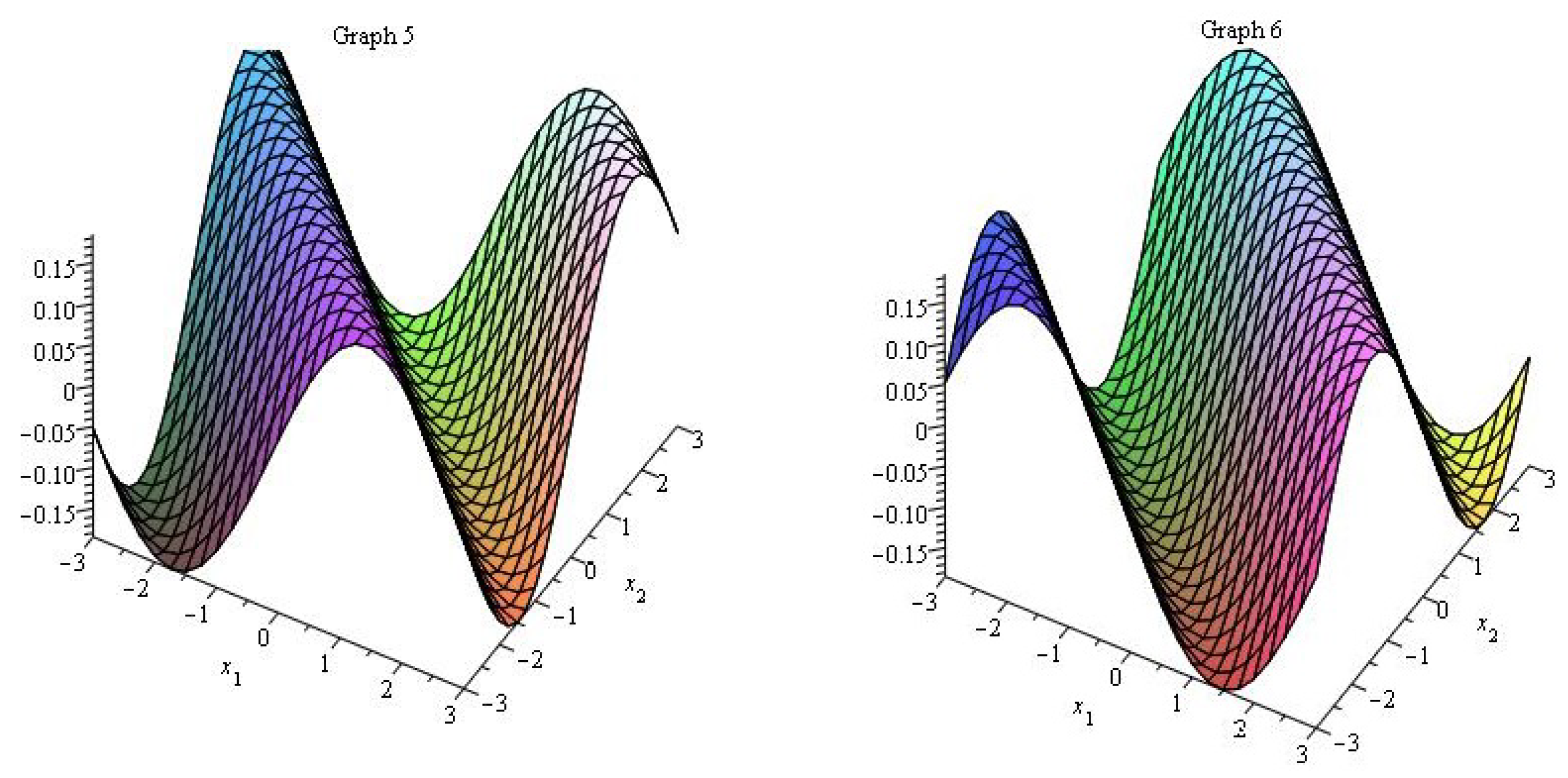
Figure 3 is consists of two graphs namely Graph 5 and Graph 6. Graph 5 and Graph 6 represents the velocity profile and of the Navier-Stokes equation respectively in example 3.1 at .
Similarly in example 3.2, the plot of two velocity profiles and for the Navier-Stoke equation are represented by Graph 7 and Graph 9 at and Graph 8 and Graph 10 at respectively.
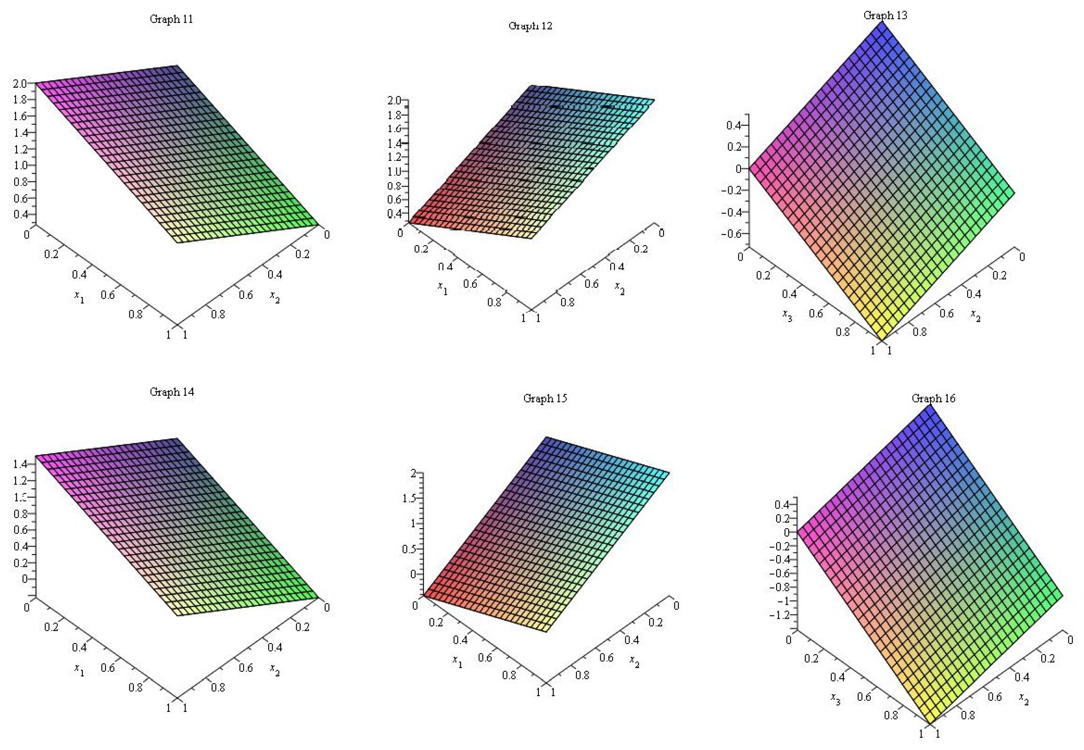
Also, in example 3.3, the plot of three velocity profiles , and for the Navier-Stoke equation are represented by Graph 11, Graph 12 and Graph 13 at and Graph 14, Graph 15 and Graph 16 at respectively.
5. Conclusions
In this paper, Laplace Adomian decomposition technique is assumed for the time-fractional classical Navier-Stokes solution of with given initial conditions. The analytical solution is given in for the power series for the given problem. The solution of the above three problems has shown, that the rate of convergence of the present method is overlapping or high than ADM and HAM. Moreover LADM have minimum calculations, simplifications as compared to ADM [12] and HPM [6].
Author Contributions
The authors have equally contributed to accomplish this research work.
Funding
Sarhad University of Science and Information Technology, Peshawar, Pakistan.
Conflicts of Interest
The authors have no conflict of interest.
References
- Khuri, S. A Laplace decomposition algorithm applied to a class of nonlinear differential equations. J. Appl. Math. 2001, 1, 141–155. [Google Scholar] [CrossRef] [Green Version]
- Ahmed, H.; Bahgat, M.; Zaki, M. Numerical approaches to system of fractional partial differential equations. J. Egypt. Math. Soc. 2017, 25, 141–150. [Google Scholar] [CrossRef]
- Jafari, H.; Khalique, C.; Nazari, M. Application of the Laplace decomposition method for solving linear and nonlinear fractional diffusion wave equations. Appl. Math. Lett. 2011, 24, 1799–1805. [Google Scholar] [CrossRef]
- Ahmad Alhendi, F.; Alderremy, A. Numerical Solutions of Three-Dimensional Coupled Burgers’ Equations by Using Some Numerical Methods. J. Appl. Math. Phys. 2016, 4, 2011–2030. [Google Scholar] [CrossRef]
- Mishra, V.; Rani, D. Newton-Raphson based modified Laplace Adomian decomposition method for solving quadratic Riccati differential equations. In Proceedings of the 4th International Conference on Advancements in Engineering & Technology, Punjab, India, 18–19 March 2016; Volume 57. [Google Scholar]
- Haq, F.; Shah, K.; Khan, A.; Shahzad, M.; Rahman, G. Numerical Solution of Fractional Order Epidemic Model of a Vector Born Disease by Laplace Adomian Decomposition Method. Punjab Univ. J. Math. 2017, 49, 13–22. [Google Scholar]
- Qasim, A.F.; AL-Rawi, E.S. Adomian Decomposition Method with Modified Bernstein Polynomials for Solving Ordinary and Partial Differential Equations. J. Appl. Math. 2018. [Google Scholar] [CrossRef]
- Yousef, H.M.; Ismail, A.M. Application of the Laplace Adomian decomposition method for solution system of delay differential equations with initial value problem. In AIP Conference Proceedings; AIP Publishing: Melville, NY, USA, 2018; Volume 1974, p. 020038. [Google Scholar]
- Rani, D.; Mishra, V. Modification of Laplace Adomian decomposition method for solving nonlinear Volterra integral and integro-differential equations based on Newton Raphson formula. Eur. J. Pure Appl. Math. 2018, 11, 202–214. [Google Scholar] [CrossRef]
- Birajdar, G. Numerical Solution of Time Fractional Navier-Stokes Equation by Discrete Adomian decomposition method. Nonlinear Eng. 2014, 3, 21–26. [Google Scholar] [CrossRef]
- Carpinteri, A.; Mainardi, F. (Eds.) Fractals and Fractional Calculus in Continuum Mechanics; Springer: Berlin, Germany, 2014; Volume 378. [Google Scholar]
- Momani, S.; Odibat, Z. Analytical solution of a time-fractional Navier–Stokes equation by Adomian decomposition method. Appl. Math. Comput. 2006, 177, 488–494. [Google Scholar] [CrossRef]
- Zhou, Y.; Peng, L. Weak solutions of the time-fractional Navier-Stokes equations and optimal control. Comput. Math. Appl. 2017, 73, 1016–1027. [Google Scholar] [CrossRef]
- Kumar, S.; Kumar, D.; Abbasbandy, S.; Rashidi, M. Analytical solution of fractional Navier-Stokes equation by using modified Laplace decomposition method. Ain Shams Eng. J. 2014, 5, 569–574. [Google Scholar] [CrossRef]
- Edeki, S.O.; Akinlabi, G.O. Coupled Method for Solving Time-Fractional Navier-Stokes Equation. Int. J. Circuits Syst. Signal Process. 2018, 12, 27–34. [Google Scholar]
- Singh, B.; Kumar, P. FRDTM for numerical simulation of multi-dimensional, time-fractional model of Navier-Stokes equation. Ain Shams Eng. J. 2016, 9, 827–834. [Google Scholar] [CrossRef]
- Ganji, Z.; Ganji, D.; Ganji, A.; Rostamian, M. Analytical solution of time-fractional Navier-Stokes equation in polar coordinate by homotopy perturbation method. Numer. Methods Part. Differ. Equ. 2010, 26, 117–124. [Google Scholar] [CrossRef]
- Hilfer, R. Applications of Fractional Calculus in Physics; World Science Publishing: River Edge, NJ, USA, 2000. [Google Scholar]
- Miller, K.S.; Ross, B. An Introduction to the Fractional Calculus and Fractional Differential Equations. 1993. Available online: http://www.citeulike.org/group/14583/article/4204050 (accessed on 29 January 2019).
- Podlubny, I. Fractional Differential Equations: An Introduction to Fractional Derivatives, Fractional Differential Equations, to Methods of Their Solution and Some of Their Applications; Elsevier: Amsterdam, The Netherlands, 1998; Volume 198. [Google Scholar]
Figure 1.
For example 1, the velocity profiles of NS equation at .

Figure 2.
For example 1, the velocity profiles of NS equation at = 0.5, q = 0, = 0.5, t = 3.

Figure 3.
For example 2, the velocity profiles of NS equation at = 0.5, q = 0, = 0.5, t = 0.05.
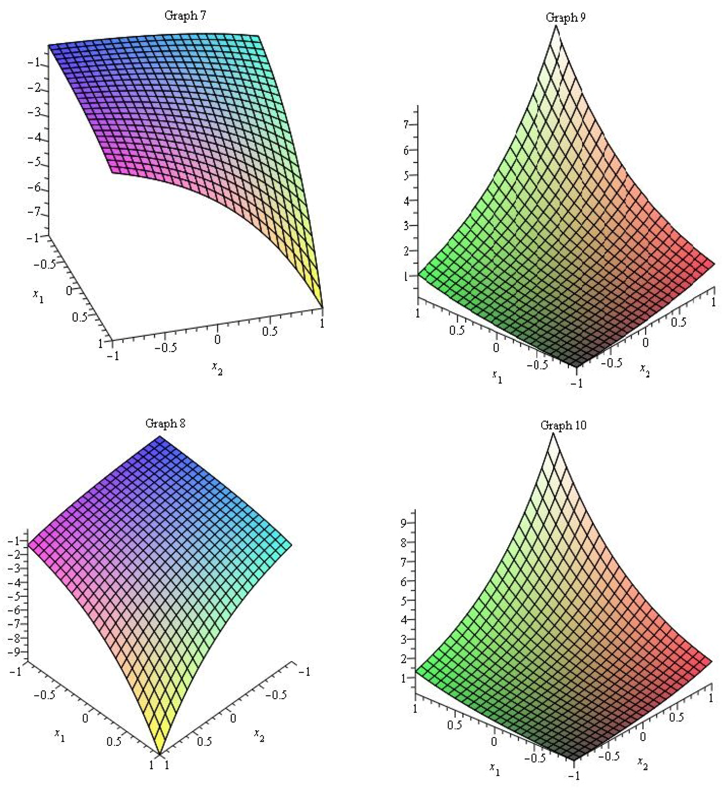
Figure 4.
For example 3, the velocity profiles of NS equation at = 0.5, = 0.5, t = 0.1.
© 2019 by the authors. Licensee MDPI, Basel, Switzerland. This article is an open access article distributed under the terms and conditions of the Creative Commons Attribution (CC BY) license (http://creativecommons.org/licenses/by/4.0/).
Share and Cite
MDPI and ACS Style
Mahmood, S.; Shah, R.; khan, H.; Arif, M. Laplace Adomian Decomposition Method for Multi Dimensional Time Fractional Model of Navier-Stokes Equation. Symmetry 2019, 11, 149. https://doi.org/10.3390/sym11020149
AMA Style
Mahmood S, Shah R, khan H, Arif M. Laplace Adomian Decomposition Method for Multi Dimensional Time Fractional Model of Navier-Stokes Equation. Symmetry. 2019; 11(2):149. https://doi.org/10.3390/sym11020149
Chicago/Turabian StyleMahmood, Shahid, Rasool Shah, Hassan khan, and Muhammad Arif. 2019. "Laplace Adomian Decomposition Method for Multi Dimensional Time Fractional Model of Navier-Stokes Equation" Symmetry 11, no. 2: 149. https://doi.org/10.3390/sym11020149
Note that from the first issue of 2016, this journal uses article numbers instead of page numbers. See further details here.