Data Source Selection Based on an Improved Greedy Genetic Algorithm

Abstract

The development of information technology has led to a sharp increase in data volume. The tremendous amount of data has become a strategic capital that allows businesses to derive superior market intelligence or improve existing operations. People expect to consolidate and utilize data as much as possible. However, too much data will bring huge integration cost, such as the cost of purchasing and cleaning. Therefore, under the context of limited resources, obtaining more data integration value is our expectation. In addition, the uneven quality of data sources make the multi-source selection task more difficult, and low-quality data sources can seriously affect integration results without the desired quality gain. In this paper, we have studied how to balance data gain and cost in the source selection, specifically, maximizing the gain of data on the premise of a given budget. We proposed an improved greedy genetic algorithm (IGGA) to solve the problem of source selection, and carried out a wide range of experimental evaluations on the real and synthetic dataset. The empirical results show considerable performance in favor of the proposed algorithm in terms of solution quality.

1. Introduction

With the continuous development of information technology, data is always being produced in all fields of modern society at all times, especially in some industries with huge data volume, such as telecommunications, transportation, medical care, securities and so on, which will generate a huge amount of data in a short period of time. To make full use of data resources and improve competitiveness in the field, policymakers need to integrate data resources and increase sources of information for deeper data analysis and mining efforts, which can bring huge benefits. However, there is no such thing as a free lunch. Data collection and integration will be costly before they bring us profit, for instance, currently emerging data platforms include Factual [1], Infochimps [2], Xignite [3], Windows Azure Data Marketplace [4], etc., which require to be paid. Even for a free and open dataset, it takes a lot of time and energy to clean up the data and solve the problem of heterogeneous data conflicts. The costs are high for individuals or companies. Therefore, in the data integration process, it is more common practice to collect data sources with high data quality and wide coverage as much as possible without exceeding the limited budget. Therefore, how to balance data integration cost and maximize integrated revenue are important issues. The existing literatures [5,6,7] have proved that the data source selection is a NP hard problem, which can be summarized as a 0–1 knapsack problem. Currently, various exact algorithms have been proposed to solve the 0–1 knapsack problem, including dynamic programming [8], core algorithms, branch and bound [9], etc. Since the solution space size of the problem is exponential with the problem input scale, these exact algorithms are not suitable for solving the larger 0–1 knapsack problem. Therefore, for the data source selection problem, a special heuristic solution is especially needed to solve the problem of selecting a suitable target source from a large amount of information sources. Heuristics are known to be classified into the following categories; binary particle swarm optimization(BPSO) [10], ant colony algorithm (ACA) [11], genetic algorithms [12], etc.

Along this line of thought, we formalized the problem of source selection as a 0–1 knapsack problem [13] and chose the appropriate solution in all possible combinations. We proposed a gain-cost model driven by data quality and used intelligent approaches to deal with this complex problem, especially with genetic algorithms (GAs). GAs, which are considered robust and efficient [14], have been widely used and are better than the methods of large-scale data analysis [15]. However, the global optimization ability and execution efficiency of genetic algorithms are often not ideal. Literature [16] believes that the reason why the genetic algorithm is not efficient to resample the points visited in the search space, is essentially caused by the randomness of genetic operators (selection, crossover, mutation). In this paper, we make appropriate improvements for these operators, and propose a novel greedy strategy to solve the source selection problem, which makes the performance of the genetic algorithm more efficient.

In short, the key contributions of this paper can be summarized as follows:

• We first summarize several dimensional indicators that affect the quality of data and establish a linear model to estimate the quality score. A gain-cost model driven by integration scores was proposed, which provides the basis for assessing the value of data sources.
• We propose an improved novel greedy genetic algorithm(IGGA). Not only improved genetic operators, but also a novel greedy strategy are proposed, which makes the source selection problem more efficient.
• We have conducted extensive experiments on real and synthetic datasets. A large number of experimental results show that our algorithm is very competitive against the other state-of-the-art intelligent algorithms in terms of performance and problem solving quality.

The remainder of this study is organized as follows. Related source selection methods and genetic algorithm in combinatorial optimization work is covered in Section 2. In Section 3, we present the problem formulation and model of the data source selection, propose the methods of data quality and source coverage estimation, and establish a gain-cost model driven by a comprehensive score. We improve the genetic operator and design an efficient greedy strategy for source selection in Section 4. We evaluate the performance of our algorithms through real and synthetic datasets in Section 5. Section 6 summarizes and discusses future research directions.

2. Related Works

2.1. The Sources Selection Approaches in a Distributed Environment

For the issue of data source selection, some classic methods have been developed. There is a wealth of literature on this topic, and then we present some of the relevant results in this area.

Much work has been done for online data consolidation, especially for source selection of deep network [17,18], but most of the work is just focused on finding the data source for a given query or domain. Such work can be summarized as a document retrieval method. Specifically, the data source is represented as a file connection or sample a document for indexing, and according to the information retrieval technology, the returned documents are classified and sorted according to the similarity of the query keywords. Then the information source is selected. Related researches include [19,20,21,22]. In recent years, people also tried to design intelligent algorithms in the field of information retrieval. Genetic algorithms are widely used to modify document descriptions, user queries, and adapt matching functions. For example [15,23,24]. However, most of these studies did not consider the impact of data source quality on the result of the source selection. Much work [25,26] focused on turning data quality standards into optimization goals for query decisions in every situation and using this information to improve the quality of query results in the data integration process. However, none of them studied the effect of source cost on the selection results. Compared with online data integration, offline data integration is less studied. Dong et al. [5] focused on the marginal revenue standard of data sources to balance data quality and integration cost. In the source selection process, the focus is to select a subset of sources for data integration, so that the overall profit of the selected source is the highest. Although they had done a great number of experimental researches, no further discussion was conducted on large sample datasets.

2.2. Application of a Genetic Algorithm in Combinatorial Optimization

As the size of the problem increases, the search space for combinatorial optimization problem also expands dramatically. Sometimes it is difficult or even impossible to find the exact optimal solution using the enumeration method on current computers. For such complex issues, people have realized that their main energy should focus on seeking the satisfied solution, and genetic algorithm is one of the best tools to find this solution. Practice has proved that the genetic algorithm has been successfully applied in solving source selection problem. Lebib et al. [27] proposed a method based on a genetic algorithm and social tagging to select, with the optimal possible way, data sources to be interrogated. Kumar et al. [28] use a genetic algorithm to select the appropriate search engine for the user query in the meta search engine. Since the user’s information needs are stored in the database of different underlying search engines, the choice of the search engine substantially improves the user’s query efficiency. Abououf et al. [29] address the problem of multi-worker multi-task selection allocation for mobile crowdsourcing, and use genetic algorithms to select the right workers for each task group, looking to maximize the QoS of the task while minimizing the distance traveled.

In addition, genetic algorithm has been applied to solve various NP-hard problems, such as the traveling salesman problem, knapsack problem, packing problem, etc. LarrNaga et al. [30] developed a genetic algorithm with different representations to tackle the travelling salesman problem. Lim et al. [31] borrowed from social monogamy: pair bonding and infidelity at a low probability and explored a pair of genetic algorithms to solve the 0–1 knapsack problem, and achieved better results. Quiroz-Castellanos et al. [32] proposed a method that was referred to the grouping genetic algorithm with controlled gene transmission to solve the bin packing problem.

To our knowledge, very few works address the problem of offline sources selection. The work of [5] is close to our work.

3. Data Source Selection Driven by the Gain-Cost Model

3.1. Problem Definition

Before defining the problem, we need to make some assumptions. We considered integrating from a set of data source S, assuming that the data integration system provided the functions of measuring cost and gain. For the cost, on the one hand, it is related to the cost of purchasing data from a specific source, depending on the pricing mechanism of the data platform. On the other hand, cost is related to data cleansing, or any other foreseen expense in the process of data integration. For such costs, historical data can be used for estimation, and the cost incurred in the data integration process can be obtained. The gain consisted of two factors, one was determined by the quality of the data source, such as the completeness and accuracy of the data, and the other was determined by the coverage [33], i.e., the data source containing the number of entities.

Before we proceed any further, it will be helpful to define a few terms. We first define some features of data source formally. Let $g_i$, $c_i$, $Q_i$, $Co{v}_i$ be the gain, cost, quality score and coverage of i-th data source. $Q_i$, $Co{v}_i$ and $g_i$ are related, and we will give a detailed explanation in the next subsection. Considering the above factors, we use $g_i$ to represent the comprehensive gain of i-th source. Then a set of data source s is given, $G\left(s\right)={\sum }_{i=1}^{\left|s\right|}{g}_i$, $C\left(s\right)={\sum }_{i=1}^{\left|s\right|}{c}_i$. Next we define the problem as follows.

Definition 1.

(Source selection) Let Ω be a set of sources, Ω = $s_1,s_2,\dots ,s_n$, and ${\delta }_c$ be a budget on cost. The source selection problem finds a subset S ⊆ Ω that maximizes $G\left(S\right)$ under constraint $C\left(S\right)$ ≤ ${\delta }_c$, which can be described as follows:

$$\begin{array}{c}MaximizeG\left(s\right)=\sum _{i=1}^{\left|s\right|}{g}_i=\sum _{i=1}^n{g}_i{x}_i\hfill \\ s.t.=\left\{\begin{array}{c}C\left(s\right)=\sum _{i=1}^{\left|s\right|}{c}_i=\sum _{i=1}^n{c}_i{x}_i\le {\delta }_c\hfill \\ x_i=0or1,i=1,2,\dots ,n\hfill \\ \left|s\right|\le n.\hfill \end{array}\right.\hfill \end{array}$$

(1)

The binary decision variable $x_i$ is used to indicate whether data source i is selected. It may be assumed that all gain and cost are positive, and that all cost is smaller than the budget ${\delta }_c$.

3.2. Data Quality and Coverage

In this paper, we considered data quality from multiple aspects. Specifically, we evaluateed quality in three areas, i.e., completeness, redundancy, accuracy, which are denoted by A, B and C respectively. Table 1 [34] contains the metrics we defined for each of the selected quality attributes, reporting names and descriptions and lists the formulas used to calculate them.

Table 1. Metric definitions, description and calculation.

Attributes	Metric	Description	Variables	Formula
Completeness	Proportion of complete cells	Indicates the proportion of complete cells in a dataset. It means the cells that are not empty and have a meaningful value assigned.	$nr$: Number of rows $nc$: Number of columns $ic$: Number of incomplete cells $ncl$: Number of cells	$ncl$ = $nr\ast nc$ $pcc$ = 1−$\frac{ic}{ncl}$
Redundancy	Proportion of duplicate records	Redundancy expresses the proportion of duplicate records in the data source. Since this factor is the cost-indicator, we convert it to the benefit-indicator.	$nr$: Number of rows $red$: Number of duplicate records	$pdc$ = 1−$\frac{red}{nr}$
Accuracy	Proportion of accurate cells	Indicate the proportion cells in a data source that has correct values according to the domain and the type of information of the data source.	$nce$: Number of cells with errors $ncl$: Number of cells	$pac$ = 1−$\frac{nce}{ncl}$

Then, we made a weighted average of these three attributes as follows:

$$\begin{array}{c}Q\left(s_i\right)=\alpha A+\beta B+\gamma C\hfill \\ s.t.\alpha +\beta +\gamma =1,\hfill \end{array}$$

(2)

where $Q\left(s_i\right)$ is the quality score of the data source $s_i$, $\alpha$, $\beta$, $\gamma$ are the weight of each attribute, which can be set by the user.

Definition 2.

(Coverage) Let$s_i$be the selected set of sources to be integrated and count the number of$s_i$containing entities as$|s_i|$. We define the coverage of$s_i$, denoted by$Cov\left(s_i\right)$, as the probability that a random entity from the world Ω. We express this probability as:

$$Cov\left(s_i\right)=\frac{|s_i|}{\mathsf{\Omega }}.$$

(3)

Example 1.

We consider data sets obtained from online bookstores. We hope to collect data on computer science books. At present, there are 894 bookstores offering a total of 1265 computer science books (each bookstore corresponds to one data provider). We pay attention to coverage, i.e., the number of books provided. After inspection, the largest data source provides 1096 books, so the coverage of the data source can be calculated to be 1096/1265 = 0.86.

Next we make some discussions for the comprehensive score of i-th source, denoted by $I\left(s_i\right)$. We analyze both data quality and coverage, and assume that they are independent of each other. The quality of data depends on the completeness, redundancy and accuracy. The coverage of data source $s_i$ is expressed in the data source containing the number of entities. On the one hand, high coverage with near zero quality should have a very low comprehensive score, and on the other hand, very high quality with near zero coverage should also have a very low comprehensive score. Therefore, its comprehensive score will be high only if the quality and coverage are both high, which is consistent with our intuition. Based on the discussions above, the comprehensive score $I\left(s_i\right)$ of i-th source is written as follows:

$$\begin{array}{c}I\left(s_i\right)=Q\left(s_i\right)\times Cov\left(s_i\right)\hfill \end{array}$$

(4)

3.3. Gain-Cost Models

We consider the impact of different gain-cost models on source selection, and adopt the comprehensive score of Section 3.2. Treat quality score and coverage as important gain factors, and establish two gain models.

• Linear gain assumes that the gain grows linearly with a certain composite score metric $I\left(s\right)$ and sets $g\left(s\right)$ = $100I\left(s\right)$
• Step gain assumes that reaching a milestone of quality will significantly increase the gain and set:

  $$g\left(s\right)=\left\{\begin{array}{cc}\hfill 100I\left(s\right)& :0\le I\left(s\right)<0.2\hfill \\ \hfill 100+100\left(I\right(s)-0.2)& :0.2\le I\left(s\right)<0.5\hfill \\ \hfill 150+100\left(I\right(s)-0.5)& :0.5\le I\left(s\right)<0.8\hfill \\ \hfill 200+100\left(I\right(s)-0.8)& :0.8\le I\left(s\right)<1\hfill \end{array}\right.$$

We assign the cost of a source in [5, 20] in two ways:

• Linear costassumes the cost grows lineraly with the $I\left(s\right)$ and applies $c\left(s\right)=15I\left(s\right)+5$;
• Step cost assumes reaching some milestone of $I\left(s\right)$ will significantly increase cost and so applies:

  $$c\left(s\right)=\left\{\begin{array}{cc}\hfill 5& :0\le I\left(s\right)<0.2\hfill \\ \hfill 10& :0.2\le I\left(s\right)<0.5\hfill \\ \hfill 15& :0.5\le I\left(s\right)<0.8\hfill \\ \hfill 20& :0.8\le I\left(s\right)\le 1\hfill \end{array}\right.$$

By randomly combining the above gain and cost models, we obtain the following four gain and cost generation models, summarized in the following Table 2.

Table 2. Gain-cost models.

	Cost	Linear	Step
Gain
Linear		L-L	L-S
Step		S-L	S-S

Meanwhile, we set the budget ${\delta }_c=\lambda {\sum }_{i=1}^{\left|s\right|}c\left(s_i\right)$, and the $\lambda$ is a random real number on $[0.3,0.6]$. In the experiment, we set $\lambda$ as 0.5.

Then we use an example to illustrate the calculational method of data source gain and cost.

Example 2.

Table 3 shows the employee information provided by one data source. First, we calculate the data quality score. According to the calculation method of data quality in Table 1, we can conclude that A is (40 − 4)/40 = 0.9, where the empty element value is four and the redundancy B is 1/5 = 0.2. This is because when the two elements of ID1 and ID9 conflict with each other, we only choose either of them. Since this factor is the cost-indicator, we convert it to the benefit-indicator, i.e., 1 − 0.2 = 0.8. Under the knowledge that the regional codes of Beijing, Shanghai and Guangzhou are 010, 021 and 020, respectively, ID3 and ID6 violate the rules. According to the formula of accuracy, C = (40 − 2)/40 = 0.95. For simplicity, we set three coefficients α, β and γ to 0.3, 0.3 and 0.4, respectively. Thus Q(s) = 0.3A + 0.3B + 0.4C = 0.9 × 0.3 + 0.8 × 0.3 + 0.95 × 0.4 = 0.89. Secondly, we calculate the comprehensive score. Here we only describe one data source. In fact, there will be multiple data sources providing employee information, assuming that all sources can provide a maximum of 10 entities, while Table 3 only provides five entities. The coverage based on Equation (3) can be calculated as 5/10 = 0.5. Thus, the comprehensive score $I\left(s_i\right)=Q\left(s_i\right)\times Cov\left(s_i\right)=0.89\times 0.5=0.445$. Finally, calculate the gain and cost of the data source based on the model provided in Section 3.3. Taking the linear gain-cost model as an example, thus g(s) = 100 × 0.445 = 44.5, c(s) = 15 × 0.445 + 5 = 11.675.

Table 3. Employee information provided by one data source.

ID	Name	Age	Sex	Status	Entry_Time	Salary	City	Area Code
1	Renata	23	F	married	2013/5	50k	Shanghai	021
3	Jeremy	36	—	married	2010/7	95k	Beijing	020
4	Armand	—	F	single	2011/6	—	Beijing	010
6	Leona	46	M	married	—	120k	Guangzhou	021
9	Renata	34	F	married	2013/5	50k	Shanghai	021

4. Improved Greedy Genetic Algorithm (IGGA)

The paper makes improvement for the genetic algorithm in the following three aspects:

4.1. Change the Way of Selection

Genetic algorithms use a variety of selection functions, including level selection, steady state selection, elite retention, and roulette-wheel selection. Some studies have shown that the roulette method is ideal for implementing selection operators and this approach enhances the chances of being suitable for chromosome selection. All solutions are placed on the roulette wheel, and a better solution has a larger portion on the roulette wheel, which provides a fair chance for each solution, and the probability of being selected is proportional to the fitness value, so individuals with higher fitness have a higher probability of survival, a higher chance of being chosen. Assuming that $M_i$ ($i=1,2,\dots ,s$) is a chromosome in a population, z is the population size, and $f\left(M_i\right)$ is the fitness of $M_i$. Fitness is expressed as the gain of the data source in Section 3.3. The selection probability ($Prob$) of each chromosome is calculated by Equation (5). The sum of probabilities from 1 to i is denoted by Equation (6).

$$Pro{b}_i=f\left(M_i\right)/\sum _{i=1}^{z}f\left(M_i\right)$$

(5)

$$Su{m}_i=\sum _{j=1}^{i}Pro{b}_j$$

(6)

Algorithm 1 describes our selection process. In order to preserve the best chromosomes, we improved the selection algorithm. All individuals in the population were ranked in descending order of fitness, with the top 1/4 of the individuals being replicated twice, the middle 2/4 individual being kept, and discarding the last 1/4. In this way, on the one hand, individuals with lower fitness can be directly eliminated, and on the other hand, the proportion of individuals with better fitness can be increased.

Algorithm 1 Selection.

input: All members of population  output: New Selected population 1 Sort all data sources in descending order of fitness; 2 The individual in the top 1/4 is copied twice, the middle 2/4 is kept, the last 1/4 is abandoned and generate a transition population; 3 Generate a random number $R\in$ [0,1]; 4 repeat 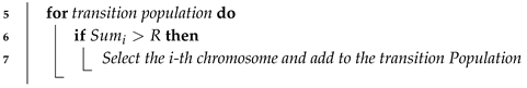8 until create offspring;

4.2. Crossover

Crossover functions were used for generation of new chromosomes. By recombining and distributing the genes on the parental chromosome to generate the children, crossover may bring together the parents’ dominant genes to produce new individuals that are more adaptive and closer to the optimal solution. We used partial-mapped crossover without “duplicates”. Thus, the gene in the generated chromosome must not be repeated. Details are given in Algorithm 2.

Algorithm 2 Crossover.

input: Parents from the current population.  output: Two new children. 1 Let M = ($m_1,m_2,\dots m_k$) and N = ($n_1,n_2\dots n_k$) two parents to crossed; 2 Choose two random number(a,b∣ a<b) on the set {1,2, …k}, two new children $\overline{M}$ and $\overline{N}$ are created according to the following rules: $$\overline{M}=\left\{\begin{array}{c}{n}_{i}if(a<i<b)\hfill \\ m_{i}otherwise\hfill \end{array}\right.\overline{N}=\left\{\begin{array}{c}{m}_{i}if(a<i<b)\hfill \\ n_{i}otherwise\hfill \end{array}\right.$$ 3 Establishing the mapping relationship in segment (a, b), f(M) ↔f(N); 4 Remove, before the cutting point(a) and after the cutting point(b), the data source which are already placed segment (a,b); 5 Put the corresponding data source on the delete location according to the mapping.

Example 3.

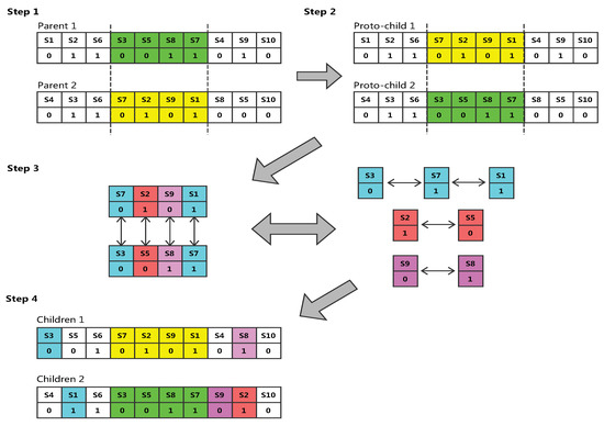
We consider 10 data sources, a flag of 1 indicates that the source was selected, a flag of 0 indicates that the source was not selected. Figure 1 shows an example of crossover.

Figure 1. Crossover operation on two selected chromosomes.

• Step 1. Randomly select the starting and ending positions of several genes in a pair of chromosomes (the two chromosomes are selected for the same position).
• Step 2. Exchange the location of these two sets of genes.
• Step 3. Detect conflict, according to the exchange of two sets of genes to establish a mapping relationship. Taking $S_3-S_7-S_1$ as an example, we can see that there are two genes $S_3$ in proto-child two in the second step, when it is transformed into the gene $S_1$ by the mapping relationship, and so on. Finally, all the conflicting genes are eliminated to ensure that the formation of a new pair of offspring genes without conflict.
• Step 4. Finally get the result.

4.3. Novel Greedy Repair Strategy

In the randomly generated initial population and each generation of genetically derived populations, there will always be some individuals who do not meet the constraints, i.e., the data source cost corresponding to their chromosomes exceeds the budget limit. A novel greedy strategy is proposed, which is named the greedy repair strategy (GRS) and given in Algorithm 3. Before the start of the algorithm, all data sources were sorted in descending order according to the ratio of comprehensive gain and cost, and the subscripts of each item were stored in array A[0⋯n] according to the sorted order. Let $Flag\left[i\right]$ be a boolean array that identifies the state of each data source. When $Flag\left[i\right]$ = 1, the data source was selected and when $Flag\left[i\right]$ = 0, it was not selected. The Algorithm 3 was first introduced in descending order of gain and cost and stored in $A\left[y_i\right]$, then we selected data sources in turn, changed $Flag\left[i\right]$ = 1, and calculated the cumulative gain and cost. It is worth mentioning that our algorithm differed from other traditional greedy algorithms in that when the cumulative cost was greater than our pre-set budget, our algorithm did not stop. Instead, the cost of the currently selected data source was subtracted from the total cost and the identification of the data source was changed to 0. In this way, the previous steps were repeated again if the cumulative cost was less than the budget until all data sources were detected. The final outputs were new chromosomes and total gain, denoted by Y and $Gain\left(Y\right)$, respectively.

Example 4.

To illustrate, we list six data sources to be selected in Table 4 and arranged them in non-ascending order of the gain-cost ratio, assuming that the budget was 100. According to the traditional greedy strategy, after selecting the source $s_3$, the algorithm will stop executing. This is because if the algorithm continues to select $s_4$, the total cost will exceed the budget. Therefore, the traditional greedy algorithm gets the total gain is (90 + 80 + 75 = 245). When using GRS, our algorithm will not stop when it executes to source $s_4$. On the contrary, GRS will skip $s_4$ and continue to evaluate source $s_5$. GRS will continue to execute until the total cost does not exceed the budget. Search for a complete list of alternate data sources. At this time, the result obtained by GRS is (90 + 80 + 75 + 45 + 10 = 300). It can been seen that GRS has an advantage over traditional greedy strategies.

Table 4. Example for greedy repair strategy (GRS).

Source	${\mathit{s}}_1$	${\mathit{s}}_2$	${\mathit{s}}_3$	${\mathit{s}}_4$	${\mathit{s}}_5$	${\mathit{s}}_6$
Flag	1	1	1	0	1	1
The ratio of gain-cost	6	4	3	2	1.5	1
Gain	90	80	75	100	45	10
Cost	15	20	25	50	30	10

Algorithm 3 Greedy repair strategy (GRS).

input: Chromosome S = [$s_1$,$s_2$,…,$s_n$], A[0…n], ${\delta }_c$: cost budget  output: A new chromosome Y = [$y_1$,$y_2$,…,$y_n$], $Gain\left(Y\right)$ 1 $y_i\leftarrow$0, $Flag\left[i\right]\leftarrow$0; 2 $Gain\leftarrow$0, $Cost\leftarrow$0, $i\leftarrow$0; 3 Arrange data sources in descending order of gain-cost ratio; 4 for ($i\lefta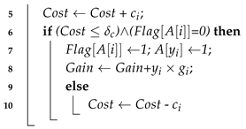rrow$ 1 to n) do 11 return (Y, $Gain\left(Y\right)$)

4.4. Integrate Greedy Strategy into GAs

Based on the above analysis, it can been seen that if GRS is used to optimize the data source selection process, not only can the problem be solved, but also the entire data source can be traversed to make the optimal solution. Next, we integrate GRS into the improved genetic algorithm, which is named IGGA. The detailed pseudocode is given in Algorithm 4.

Algorithm 4 Improved greedy genetic algorithm (IGGA).

input: $S=\{s_1,s_2,\cdots ,s_n\}$,     G = {($g_1$,$g_2$,$g_i$, …, $g_n$)|( 0≤ i ≤ n)},     C = {($c_1$,$c_2$,$c_i$, …, $c_n$)| (0≤ i ≤ n)},     Z, $p_c$, $p_m$, $MaxIt$  output: Optimal solution $S\left(r\right)$, Objective gain value $f\left(S\right(r\left)\right)$ 1 A[0…n]←Descending{$g_i$ / $c_i$ | $g_i$∈ G, $c_i$∈ C, (0 ≤ i ≤ n)}; 2 Generate randomly an initial population of P = {$S_i$(0) | 1 ≤ i ≤ Z}; 3 for i← 1 to Z do 5 Set the number of inner loops r ← 0; 6 while (r ≤ $Ma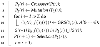xIt$) do 14 return $S\left(r\right)$, $f\left(S\right(r\left)\right)$;

The genetic algorithm based on the above greedy strategy is as follows:

• Step 1. According to the greedy repair strategy, all the selected data sources are non-incrementally sorted according to the ratio of gain and cost.
• Step 2. Use the binary coding method, randomly generate the initial population P, and use the greedy strategy to obtain the initial current optimal solution.
• Step 3. The fitness is calculated for each chromosome in the population P, and if the value corresponding to the chromosome is greater than the current optimal solution, the current solution is replaced.
• Step 4. If the maximum number of iterations is reached, then stop. Otherwise, a crossover operation is performed, and a temporary population $P_1\left(r\right)$ is obtained according to the crossover probability.
• Step 5. With a small probability $p_m$, a certain gene of each chromosome is mutated, and then a temporary population $P_2\left(r\right)$ is generated. Use greedy strategies to repair chromosomes that do not meet the constraints.
• Step 6. Select some chromosomes according to Equation (5) to form a new population $P(r+1)$, and turn to Step 3.

In our algorithm, genetic operations (i.e., selection, crossover, mutation) further explored and utilized more combinations to optimize the objective function, while the greedy repair strategy not only improved the efficiency of the algorithm, but also evaluated whether each candidate data source met the constraints, so as to obtain high-quality solutions.

5. Experimental Design and Result

5.1. Experimental Design

This section will include algorithm parameter settings, and a number of comparative and verification experiment listed below:

• To make the comparison as fair as possible, we discussed the trend of IGGA parameter values under the four gain-cost models and set reasonable values for them.
• We compared the average performance and the stability of IGGA, DGGA [35], BPSO [10] and ACA [11] in a real data set.
• We compared the performance of IGGA and DGGA in the synthetic data set. In addition, we made comparisons with other state-of-the-art intelligent algorithms to verify the efficiency of IGGA.

All experiments were coded in Python under Windows 10 for Education platform on an Intel Core i7 2.8 GHz processor with 8 GB of RAM.

5.1.1. Dataset

We employed both real and synthetic datasets in the experimental evaluations.

We experimented on two data sets, i.e., Book and Flight [36]. The Book contained 894 data sources, which were registered with AbeBooks.com and in 2007 provided information on computer science books. They provided a total of 12,436 books, with ISBNs, names, and authors. The data source coverage provided was from 0.1% to 86%. The Flight collected information of over 1200 flights from 38 sources over a one-month period, together providing more than 27,000 records, each source providing 1.6% to 100% of the flights.

In addition, we used the classic datasets of the 0–1 knapsack problem, which were provided by [37,38]. The size of these datasets was less than 40 problem instances. Here, we called these small-S. Meanwhile, according to the method provided by [37], we also randomly generated eight instance sets ranging from 100 to 1500, which were called large-S.

5.1.2. Parameter Settings

In the experiment, two data sets were applied to four gain-cost models and eight data instances were generated. Since the IGGA is a kind of parameter-sensitive evolutionary algorithm, crossover operation and mutation operation played key roles in the generation of new solutions. Many researches [39] have shown that it is difficult to search forward when the crossover probability $p_c$ is too small, and it is easy to destroy the high fitness structure. When the mutation probability $p_m$ is too low, it is difficult to generate a new gene structure. Conversely, if $p_m$ is too high, GA becomes a simple random search. To further investigate the optimal values of $p_c$ and $p_m$ in IGGA, we solved eight instances by IGGA to determine the values of $p_c$ and $p_m$.

Specifically, we set $p_c$ to (0.1, 0.3, 0.5, 0.7, 0.9), and $p_m$ to (0.01, 0.05, 0.1, 0.3, 0.5, 0.7, 0.9), respectively. As a result, we got a total of 35 different combinations ($p_c$, $p_m$), and an ID was assigned to each combination, which are shown in Table 5. Once the range of parameters was determined, the different combinations of parameters on each gain-cost model was independently calculated 30 times. Finally, we got a performance comparison of IGGA with 35 parameters on the four gain-cost models (in Section 4). According to Figure 2 and Figure 3, it is easy to see that $p_c$ = 0.5 and $p_m$ = 0.01 are the most reasonable choices.

Table 5. The 35 different combinations of crossover and mutation probabilities.

ID	$({\mathit{p}}_{\mathit{c}},{\mathit{p}}_{\mathit{m}})$	ID	$({\mathit{p}}_{\mathit{c}},{\mathit{p}}_{\mathit{m}})$	ID	$({\mathit{p}}_{\mathit{c}},{\mathit{p}}_{\mathit{m}})$	ID	$({\mathit{p}}_{\mathit{c}},{\mathit{p}}_{\mathit{m}})$	ID	$({\mathit{p}}_{\mathit{c}},{\mathit{p}}_{\mathit{m}})$
1	$(0.1,0.01)$	8	$(0.3,0.01)$	15	$(0.5,0.01)$	22	$(0.7,0.01)$	29	$(0.9,0.01)$
2	$(0.1,0.05)$	9	$(0.3,0.05)$	16	$(0.5,0.05)$	23	$(0.7,0.05)$	30	$(0.9,0.05)$
3	$(0.1,0.1)$	10	$(0.3,0.1)$	17	$(0.5,0.1)$	24	$(0.7,0.1)$	31	$(0.9,0.1)$
4	$(0.1,0.3)$	11	$(0.3,0.3)$	18	$(0.5,0.3)$	25	$(0.7,0.3)$	32	$(0.9,0.3)$
5	$(0.1,0.5)$	12	$(0.3,0.5)$	19	$(0.5,0.5)$	26	$(0.7,0.5)$	33	$(0.9,0.5)$
6	$(0.1,0.7)$	13	$(0.3,0.7)$	20	$(0.5,0.7)$	27	$(0.7,0.7)$	34	$(0.9,0.7)$
7	$(0.1,0.9)$	14	$(0.3,0.9)$	21	$(0.5,0.9)$	28	$(0.7,0.9)$	35	$(0.9,0.9)$

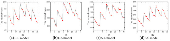
Figure 2. Performance comparison of four gain-cost models with 35 combinations (Book dataset).

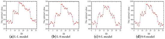
Figure 3. Performance comparison of four gain-cost models with 35 combinations (Flight dataset).

When eight instances are solved with IGGA, DGGA, BPSO, ACA, the population size of all algorithms is set to 30 and the number of iterations is set to 300. In DGGA, uniform crossover operation, directional mutation operation and elite selection strategy are used; the crossover probability $p_c$ = 0.8, and the mutation probability $p_m$ = 0.15. In BPSO, set W = 0.8, $C_1$ = $C_2$ = 1.5. In ACA, the pheromone trace is set to $\alpha$ = 1.0, the heuristic factor $\beta$ =1.0, the volatile factor $\rho$ = 0.7.

5.2. Experimental Results

5.2.1. Performance Comparison of Four Algorithms under Different Gain-Cost Models Using Real Datasets

We used Book and Flight datasets and generated a total of eight instances based on four gain-cost models. IGGA, DGGA, BPSO, ACA were used to obtain the best value, the worst value, the mean value, the standard deviation (S.D), and the time for solving each instance 30 times independently. Time represents the average running time required for each algorithm to solve each instance separately.

As can be seen from Table 6, IGGA achieved the best results in five of the eight instances, DGGA did that in two instances, BPSO achieved the best results on only one instance, while ACA did not. Regarding the average running time, the solution speed of DGGA and IGGA were almost equal, significantly faster than BPSO and ACA. The difference between the speed of the BPSO and ACA was small.

Table 6. Performance comparison of improved greedy genetic algorithm (IGGA), DGGA, BPSO and ACA.

Datasets	Index	Gain	Cost	Algorithm	Best	Mean	Worst	S.D	Time
Book	1	Linear	Linear	IGGA	986.32	963.16	921.41	6.84	2.423
				DGGA	953.16	921.84	886.62	13.89	2.218
				BPSO	911.64	863.71	838.50	14.22	3.135
				ACA	935.55	896.39	865.04	16.49	3.352
	2		Step	IGGA	1092.21	1041.62	989.58	9.58	1.883
				DGGA	967.08	894.21	847.33	11.98	1.684
				BPSO	988.36	918.48	843.24	16.69	2.418
				ACA	1013.14	968.74	921.37	12.99	2.350
	3	Step	Linear	IGGA	2052.45	1988.17	1923.62	8.73	2.045
				DGGA	2037.22	1942.46	1890.54	8.94	1.976
				BPSO	2055.86	1968.04	1904.88	15.83	2.724
				ACA	2011.37	1904.32	1852.56	18.48	2.831
	4		Step	IGGA	1926.05	1868.74	1831.81	7.17	1.928
				DGGA	1902.28	1828.79	1787.03	9.89	1.882
				BPSO	1908.45	1803.86	1762.26	13.92	2.281
				ACA	1895.32	1789.92	1723.04	17.34	2.292
Flight	1	Linear	Linear	IGGA	436.77	417.62	394.17	6.35	0.116
				DGGA	421.21	396.45	376.35	8.06	0.102
				BPSO	413.58	388.39	369.67	11.20	0.185
				ACA	405.18	384.35	374.58	7.47	0.206
	2		Step	IGGA	465.26	437.72	421.28	5.58	0.108
				DGGA	472.16	431.31	415.84	7.92	0.112
				BPSO	442.04	406.46	381.26	10.52	0.168
				ACA	416.37	390.61	373.92	8.96	0.179
	3	Step	Linear	IGGA	1105.54	1062.48	970.14	11.64	0.227
				DGGA	1045.34	991.67	966.38	8.95	0.198
				BPSO	992.32	936.72	893.15	10.40	0.294
				ACA	1019.93	958.61	902.94	13.94	0.315
	4		Step	IGGA	964.15	908.23	870.66	7.88	0.206
				DGGA	972.37	902.52	862.17	10.95	0.192
				BPSO	911.63	858.35	810.81	14.75	0.308
				ACA	902.46	852.58	803.96	15.56	0.336

Since the heuristic algorithm is a random approximation algorithm, to evaluate its performance, we used the $GAP$ metric in [40] to evaluate the average performance statistics of all algorithms. Specifically, $GAP$ represents the relative difference between the best value and the mean value, i.e., $GAP=\frac{|best-mean|}{best}\times 100\%$. It can compare the average performance of all algorithms by fitting curves. If the $GAP$ curve is closer to the abscissa axis, the average performance of the algorithm is better. From Figure 4a,b, it can be seen that among the four algorithms, the average performance of IGGA is the best, because the $GAP$ curve is the closest to the abscissa axis.

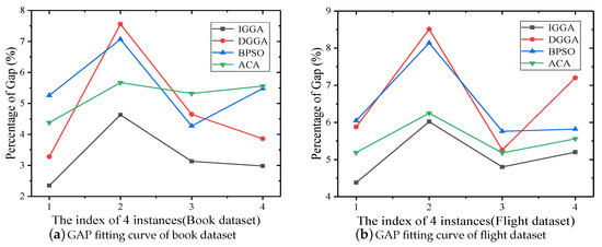
Figure 4. $GAP$ fitting curve of two data sets under four gain-cost models.

Moreover, in order to evaluate the stability of the algorithm, we drew a histogram based on the value of S.D and evaluated the stability of all algorithms by the distribution of the columns. Figure 5a,b show that the stability of IGGA and DGGA was roughly equal in all algorithms, but significantly higher than BPSO and ACA.

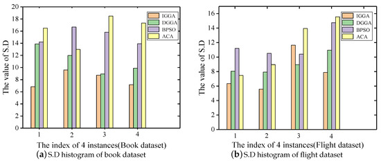
Figure 5. Standard deviation (S.D) histogram of two data sets under four gain-cost models.

5.2.2. Performance Comparison of Algorithms under Different Source Scales Using Synthetic Datasets

To investigate the scalability of the algorithm, we adapted the synthetic dataset, and evaluated the performance of IGGA through extensive experimentation. According to literature [37], we divided the dataset into two parts. The instances labeled 1–12 as small-S, and the instances labeled 13–20 as large-S. The IGGA and DGGA solutions are shown in Table 7.

Table 7. The best value, the worst value, mean optima, and S.D for comparison between IGGA and DGGA.

Algorithm			IGGA				DGGA
ID	Scale	Best	Worst	Mean	S.D	Best	Worst	Mean	S.D
1	10	295	295	295	0	295	288	292.32	1.24
2	20	1024	1024	1024	0	1024	1024	1024	0
3	4	35	35	35	0	35	28	34.58	1.56
4	4	23	23	23	0	23	23	23	0
5	15	481.07	481.07	481.07	0	481.07	438.24	478.57	9.38
6	10	50	50	50	0	50	40	46.8	1.96
7	7	107	107	107	0	107	93	106.2	1.38
8	23	9776	9776	9776	0	9767	9754	9766.32	0.76
9	5	130	130	130	0	130	130	130	0
10	20	1025	1025	1025	0	1025	1025	1025	0
11	30	5786	5380	5765	32.63	5716	5245	5560	54.47
12	40	4994	3857	4903	18.25	4994	3548	3742	35.82
13	100	6983	6854	6938.23	16.92	6879	6781	6857.34	20.57
14	200	10,799	10,677	10,731.22	23.42	10,522	10,282	10,358.73	36.45
15	300	13,368	13,104	13,271.94	54.04	12,566	12,362	12,472.45	75.54
16	500	18,111	17,684	17,878.74	92.34	17,921	17,450	17,743.37	146.08
17	800	37,338	36,892	37,172.17	114.16	35,147	34,741	34,914.81	189.47
18	1000	64,847	64,315	64,533.04	136.37	60,132	58,994	59,628.06	285.26
19	1200	86,399	85,847	86,142.41	88.17	86,003	85,224	85,647.24	352.06
20	1500	101,556	101,214	101,427.26	64.34	98,862	97,938	98,575.67	465.23

The best value, the mean value, the worst value and the S.D were collected for IGGA and DGGA over 30 independent runs, which are tabulated in Table 7.

As can be seen in Table 7, for 12 small scale problem instances, IGGA had an advantage over DGGA, and there were six values superior to DGGA in the mean measure, and no difference for the remaining tests. The problem set appeared to be less challenging as both algorithms were able to reach optima in most of the cases with little difficulties.

If the quality of the IGGA solution was not surprising at the small-scale problem instance; let’s look at the performance of the large-scale problem. For instance 13–20, the IGGA has demonstrated an overwhelming advantage over DGGA. The worst solution discovered by IGGA was even better than the best solution obtained by DGGA, e.g., (14, 15, 17, 18, 20). In addition, in view of stability and consistency in finding optima, the proposed algorithm clearly surpassed DGGA with its smaller standard deviations for all problem instances. In short, IGGA has demonstrated better performance when solving source selection problems than DGGA.

5.2.3. Convergence Analysis

We have chosen two representative instances, (i.e., instance 11 and instance 16), and we also plot the solution quality of the two algorithms, as shown in Figure 6a,b. DGGA converged to local optima very quickly. However, IGGA started off slowly at the early stage of evolution due to the following two reasons. Firstly, the evolutionary process of IGGA needed to sort the ratio of gain and cost according to the early quick sorting algorithm. Secondly, our greedy strategy required traversal of all data sources, all of which required time. After undergoing crossover and mutation operations, GRS further explored other unknown areas to improve performance and generate better solutions. It can be seen that the IGGA solution was more effective than DGGA. This was the same for small-scale instance 11 and large-scale instance 16.

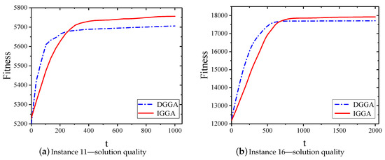
Figure 6. Sample convergence plots for problem instances 11 and 16.

In fact, for large-scale instances, IGGA was not materially impacted by the large gain and cost factors, and we compared the gain-cost ratio, which simplified the problem to a new set of instances. Meanwhile, it was more in line with the demand of the solution in a practical application, so as to obtain a balance between solution quality and convergence rate.

5.2.4. Comparison with Other State-of-the-Art Models

Table 8 shows the experimental comparison of IGGA for 10 small-scale instances with previous research work. Among them, the bold represents the best optimization result, and the dash (—) indicates that the item had not been tested. In this table, we do not list the comparison results of large-scale instances, because the instance problems were randomly generated, and different experiment settings had different instance problem sets. It can be seen that IGGA was highly competitive with the most advanced methods from Table 8. IGGA can find the best value of the problem, except for instance 6, and it is especially worth mentioning that in instance 8, it found a new optimal optimization value.

Table 8. Comparing the experimental results with other state-of-the-art approaches.

ID	Instance	IGGA	MopGA [31]	Harmony Algorithm [37]	AOA [41]
1	10	295	295	295	295
2	20	1024	1024	1024	—
3	4	35	35	35	35
4	4	23	23	23	23
5	15	481.07	481.07	481.07	—
6	10	50	52	50	52
7	7	107	107	107	107
8	23	9776	9767	9767	—
9	5	130	130	130	130
10	20	1025	1025	1025	—

6. Conclusions and Future Work

This paper studies the data source selection problem of maximizing revenue. We used data completeness, redundancy, accuracy and data coverage as evaluation indicators to establish a gain-cost model and proposed an improved greedy genetic algorithm. The selection operation and crossover operation have been improved. Finally, we conducted extensive experimental evaluations on real data set and synthetic data. The results have shown that our algorithm has efficient performance and wide applicability. The proposed method provided a new idea for data source selection.

In the future work, first, we will consider an efficient and comprehensive method to estimate data quality, propose a more complete data quality evaluation system, and select these new measures. The second step is to develop more effective source selection methods. The last is to establish a complex gain-cost model. When the data quality is multidimensional, the revenue model can be more complex.

References

- Factual. Available online: https://www.factual.com/ (accessed on 5 January 2019).
- Infochimps. Available online: http://www.infochimps.com/ (accessed on 5 January 2019).
- Xignite. Available online: http://www.xignite.com/ (accessed on 27 December 2018).
- Microsoft Windows Azure Marketplace. Available online: https://azuremarketplace.microsoft.com/en-us/ (accessed on 8 January 2019).
- Dong, X.L.; Saha, B.; Srivastava, D. Less is More: Selecting Sources Wisely for Integration. Proc. VLDB Endow. 2012, 6, 37–48. [Google Scholar] [CrossRef]
- Rekatsinas, T.; Dong, X.L.; Srivastava, D. Characterizing and Selecting Fresh Data Sources. In Proceedings of the 2014 ACM SIGMOD International Conference on Management of Data (SIGMOD ’14), Snowbird, UT, USA, 22–27 June 2014; pp. 919–930. [Google Scholar]
- Lin, Y.; Wang, H.; Zhang, S.; Li, J.; Gao, H. Efficient Quality-Driven Source Selection from Massive Data Sources. J. Syst. Softw. 2016, 118, 221–233. [Google Scholar] [CrossRef]
- Martello, S.; Pisinger, D.; Toth, P. Dynamic Programming and Strong Bounds for the 0–1 Knapsack Problem. Manag. Sci. 1999, 45, 414–424. [Google Scholar] [CrossRef]
- Martello, S.; Pisinger, D.; Toth, P. New Trends in Exact Algorithms for the 0-1 Knapsack Problem. Eur. J. Oper. Res. 2000, 123, 325–332. [Google Scholar] [CrossRef]
- Chand, J.; Deep, K. A Modified Binary Particle Swarm Optimization for Knapsack Problems. Appl. Math. Comput. 2012, 218, 11042–11061. [Google Scholar]
- He, L.; Huang, Y. Research of ant colony algorithm and the application of 0-1 knapsack. In Proceedings of the 2011 6th International Conference on Computer Science & Education (ICCSE), Singapore, 3–5 August 2011; pp. 464–467. [Google Scholar]
- Goldberg, D.E. Genetic Algorithms in Search, Optimization and Machine Learning; Addison-Wesley: Hoboken, NJ, USA, 1989. [Google Scholar]
- Zhao, J.; Huang, T.; Pang, F.; Liu, Y. Genetic Algorithm Based on Greedy Strategy in the 0-1 Knapsack Problem. In Proceedings of the 2009 Third International Conference on Genetic and Evolutionary Computing, Guilin, China, 14–17 October 2009; pp. 105–107. [Google Scholar]
- Kallel, L.; Naudts, B.; Rogers, A. Theoretical Aspects of Evolutionary Computing; Springer-Verlag: Berlin, Germany, 2013. [Google Scholar]
- Drias, H.; Khennak, I.; Boukhedra, A. A hybrid genetic algorithm for large scale information retrieval. In Proceedings of the 2009 IEEE International Conference on Intelligent Computing and Intelligent Systems, Shanghai, China, 20–22 November 2009; pp. 842–846. [Google Scholar]
- Salomon, R. Improving the Performance of Genetic Algorithms through Derandomization. Softw. Concepts Tools 1997, 18, 175–199. [Google Scholar]
- Balakrishnan, R.; Kambhampati, S. Factal: Integrating Deep Web Based on Trust And relevance. In Proceedings of the 20th International Conference on World Wide Web, WWW 2011, Hyderabad, India, 28 March–1 April 2011; pp. 181–184. [Google Scholar]
- Calì, A.; Straccia, U. Integration of Deepweb Sources: A Distributed Information Retrieval Approach. In Proceedings of the 7th International Conference on Web Intelligence, Mining and Semantics, Amantea, Italy, 19–22 June 2017; pp. 1–4. [Google Scholar]
- Nuray, R.; Can, F. Automatic Ranking of Information Retrieval Systems Using Data Fusion. Inf. Process. Manag. 2006, 42, 595–614. [Google Scholar] [CrossRef]
- Xu, J.; Pottinger, R. Integrating Domain Heterogeneous Data Sources Using Decomposition Aggregation Queries. Inf. Syst. 2014, 39, 80–107. [Google Scholar] [CrossRef]
- Moreno-Schneider, J.; Martínez, P.; Martínez-Fernández, J.L. Combining heterogeneous sources in an interactive multimedia content retrieval model. Expert Syst. Appl. 2017, 69, 201–213. [Google Scholar] [CrossRef]
- Abel, E.; Keane, J.; Paton, N.W.; Fernandes, A.A.A.; Koehler, M.; Konstantinou, N.; Cesar, J.; Rios, C.; Azuan, N.A.; Embury, S.M. User Driven Multi-Criteria Source Selection. Inf. Sci. 2018, 431, 179–199. [Google Scholar] [CrossRef]
- Al Mashagba, E.; Al Mashagba, F.; Nassar, M.O. Query Optimization Using Genetic Algorithms in the Vector Space Model. arXiv, 2011; arXiv:1112.0052. [Google Scholar]
- Araujo, L.; Pérez-Iglesias, J. Training a Classifier for the Selection of Good Query Expansion Terms with a Genetic Algorithm. In Proceedings of the IEEE Congress on Evolutionary Computation, Barcelona, Spain, 18–23 July 2010. [Google Scholar]
- Sun, M.; Dou, H.; Li, Q.; Yan, Z. Quality Estimation of Deep Web Data Sources for Data Fusion. Procedia Eng. 2012, 29, 2347–2354. [Google Scholar] [CrossRef]
- Nguyen, H.Q.; Taniar, D.; Rahayu, J.W.; Nguyen, K. Double-Layered Schema Integration of Heterogeneous XML Sources. J. Syst. Softw. 2011, 84, 63–76. [Google Scholar] [CrossRef]
- Lebib, F.Z.; Mellah, H.; Drias, H. Enhancing Information Source Selection Using a Genetic Algorithm and Social Tagging. Int. J. Inf. Manag. 2017, 37, 741–749. [Google Scholar] [CrossRef]
- Kumar, R.; Singh, S.K.; Kumar, V. A Heuristic Approach for Search Engine Selection in Meta-Search Engine. In Proceedings of the International Conference on Computing, Communication & Automation, Noida, India, 15–16 May 2015; pp. 865–869. [Google Scholar]
- Abououf, M.; Mizouni, R.; Singh, S.; Otrok, H.; Ouali, A. Multi-worker multitask selection framework in mobile crowd sourcing. J. Netw. Comput. Appl. 2019. [Google Scholar] [CrossRef]
- Larr Naga, P.; Kuijpers, C.M.H.; Murga, R.H.; Inza, I.; Dizdarevic, S. Genetic Algorithms for the Travelling Salesman Problem: A Review of Representations and Operators. Artif. Intell. Rev. 1999, 13, 129–170. [Google Scholar] [CrossRef]
- Lim, T.Y.; Al-Betar, M.A.; Khader, A.T. Taming the 0/1 Knapsack Problem with Monogamous Pairs Genetic Algorithm. Expert Syst. Appl. 2016, 54, 241–250. [Google Scholar] [CrossRef]
- Quiroz-Castellanos, M.; Cruz-Reyes, L.; Torres-Jimenez, J.; Claudia Gómez, S.; Huacuja, H.J.F.; Alvim, A.C.F. A Grouping Genetic Algorithm with Controlled Gene Transmission for the Bin Packing Problem. Comput. Oper. Res. 2015, 55, 52–64. [Google Scholar] [CrossRef]
- Sarma, A.D.; Dong, X.L.; Halevy, A. Data Integration with Dependent Sources. In Proceedings of the 14th International Conference on Extending Database Technology, Uppsala, Sweden, 21–24 March 2011. [Google Scholar]
- Vetrò, A.; Canova, L.; Torchiano, M.; Minotas, C.O.; Iemma, R.; Morando, F. Open Data Quality Measurement Framework: Definition and Application to Open Government Data. Gov. Inf. Q. 2016, 33, 325–337. [Google Scholar] [CrossRef]
- Liu, W.; Liu, G. Genetic Algorithm with Directional Mutation Based on Greedy Strategy for Large-Scale 0–1 Knapsack Problems. Int. J. Adv. Comput. Technol 2012, 4, 66–74. [Google Scholar] [CrossRef]
- The Book and Flight datasets. Available online: http://lunadong.com/fusionDataSets.htm (accessed on 13 October 2018).
- Zou, D.; Gao, L.; Li, S.; Wu, J. Solving 0-1 Knapsack Problem by a Novel Global Harmony Search Algorithm. Appl. Soft Comput. J. 2011, 11, 1556–1564. [Google Scholar] [CrossRef]
- Pospichal, P.; Schwarz, J.; Jaros, J. Parallel Genetic Algorithm Solving 0/1 Knapsack Problem Running on the GPU. Mendel 2010, 1, 64–70. [Google Scholar]
- Srinivas, M.; Patnaik, L.M. Adaptive Probabilities of Crossover and Mutation in Genetic Algorithms. IEEE Trans. Syst. Man Cybern. 1994, 24, 656–667. [Google Scholar] [CrossRef]
- He, Y.; Wang, X. Group theory-based optimization algorithm for solving knapsack problems. Knowl.-Based Syst. 2018. [Google Scholar] [CrossRef]
- Zhang, X.; Huang, S.; Hu, Y.; Zhang, Y.; Mahadevan, S.; Deng, Y. Solving 0-1 Knapsack Problems Based on Amoeboid Organism Algorithm. Appl. Math. Comput 2013, 219, 9959–9970. [Google Scholar] [CrossRef]
© 2019 by the authors. Licensee MDPI, Basel, Switzerland. This article is an open access article distributed under the terms and conditions of the Creative Commons Attribution (CC BY) license (http://creativecommons.org/licenses/by/4.0/).