Imaginary Chemical Potential, NJL-Type Model and Confinement–Deconfinement Transition

Abstract

In this review, we present of an overview of several interesting properties of QCD at finite imaginary chemical potential and those applications to exploring the QCD phase diagram. The most important properties of QCD at a finite imaginary chemical potential are the Roberge–Weiss periodicity and the transition. We summarize how these properties play a crucial role in understanding QCD properties at finite temperature and density. This review covers several topics in the investigation of the QCD phase diagram based on the imaginary chemical potential.

1. Introduction

Understanding nonperturbative properties of quantum chromodynamics (QCD) at finite temperature (T) and chemical potential ($\mu$) is one of the important and interesting subjects in the elementary particle, nuclear and hadron physics. The confinement–deconfinement transition and the chiral phase transition are famous examples of the properties. To investigate the non-perturbative features of QCD, the lattice QCD simulation is the powerful and gauge invariant approach, but it has the well-known sign problem at finite real chemical potential, $\mu =({\mu }_{\mathrm{R}},0)$, and thus we cannot perform it exactly in the region. Several methods are proposed so far to circumvent the sign problem, see Ref. [1] as an example, but the applicable regions are still limited in ${\mu }_{\mathrm{R}}/T<1$. It should be noted that there are some attempts to overcome the limitation: famous methods are the complex Langevin method [2,3], the Lefschetz thimble method [4,5,6], the path optimization method [7,8] and so on. However, these methods still have serious problems.

Because of the sign problem, low energy effective models of QCD are widely used to explore the QCD phase diagram. The Nambu–Jona–Lasinio (NJL) model is one of the famous low energy effective models of QCD; it can describe the spontaneous chiral symmetry breaking and also its restoration. However, this model cannot describe another important nonperturbative property of QCD, i.e., the confinement phenomena. In Ref. [9], however, the author introduces the Polyakov loop which becomes the order parameter of the confinement–deconfinement transition in the pure Yang–Mills theory to the NJL model and then the door for discussions of the confinement–deconfinement transition in the QCD effective model has been opened; this model, which can describe the chiral phase transition and the approximated confinement–deconfinement transition, is called the Polyakov-loop extended NJL (PNJL) model. It should be noted that there are some other approaches which can treat these properties such as the Dyson-Schwinger equation, the functional renormalization group and the covariant spectator theory; see Refs. [10,11,12,13].

The Polyakov loop which is related with the gauge invariant holonomy is the order parameter of the spontaneous ${\mathbb{Z}}_3$ (center) symmetry breaking in the pure Yang–Mills theory. The definition of the Polyakov loop is

$$\begin{array}{c}\hfill \mathsf{\Phi }:=\frac{1}{N_{\mathrm{c}}}\mathrm{Tr}L,L=\mathcal{P}exp\left(i{\int }_0^{\beta }d\tau A_4(\tau ,\mathbf{x})\right),\end{array}$$

(1)

where $N_{\mathrm{c}}$ is the number of color, $\beta$ does the inverse temperature ($1/T$) and $\mathcal{P}$ represents the path ordering. The Polyakov loop can be expressed in the pure Yang–Mills theory as $\mathsf{\Phi }\sim e^{-\beta F_q},$ where $F_q$ means the one-quark excitation free energy. Therefore, $\mathsf{\Phi }=0$ means the confined phase because we need the infinite $F_q$ to pick up the single quark from the thermal system. In comparison, we can pick up the single quark from the system when $\mathsf{\Phi }$ is nonzero; it is nothing but the deconfined phase. Of course, the ${\mathbb{Z}}_3$ symmetry is explicitly broken when the dynamical quarks are taken into account in the system and then the relationship between the Polyakov loop and the free energy becomes unclear. However, we are still expecting that the Polyakov loop can represent some parts of the confinement phenomena in the dynamical quark system. Actually, the PNJL model with some modifications can well reproduce states-of-arts lattice QCD data at finite T; for example, see Ref. [14] as an example and also see Refs. [15,16,17,18,19] for some lattice data. Although effective models of QCD can provide us several important and interesting pieces of knowledge, such effective models have large model ambiguities. Thus, quantitative predictions are impossible at present. Particularly, ambiguities become serious at moderate and high density regions because we cannot access the lattice QCD data in the region because of the sign problem. This indicates that we need some more approaches to remove model ambiguities to quantitatively discuss nonperturbative natures of QCD at finite density when we employ the effective models of QCD.

The imaginary chemical potential, $\mu =(0,{\mu }_{\mathrm{I}})$, which may cause readers to feel the strange sound, but this region is the promising laboratory to remove the ambiguities of the effective models of QCD. This region has the following desirable properties:

• Sign problem free,
• Possible analytic continuation process to the real chemical potential,
• Relationship with the real chemical potential region via the canonical ensemble.

These properties open the door to remove the model ambiguities, particularly ambiguities induced from the chemical potential effects. The importance of the imaginary chemical potential region can be understood from the canonical ensemble method [20,21,22,23,24] which is related with list 3; the grand-canonical partition function with $\mu =(0,{\mu }_{\mathrm{R}})$ can be obtained from the grand-canonical partition function with $\mu =(0,{\mu }_{\mathrm{I}})$ via the Fourier transformation and the fugacity expansion [25]. This fact means that the imaginary chemical potential region has almost all of information of the real chemical potential region. Details are explained later.

In addition to the sign problem, the imaginary chemical potential may provide us with important and interesting knowledge about the confinement phenomena: in ordinary understanding of the confinement–deconfinement transition at a finite temperature in QCD, there are no “phase transitions”, i.e., the crossover; there are no singularities in local order-parameters and also the thermodynamic quantities. However, it has been recently discussed in Ref. [26] that the confinement and deconfinement states at zero temperature can be clarified via the topological order [27] and then it is not necessary that the local order-parameter exists and several observable show singular behaviors. The analogy of the topological order has been applied to the thermal QCD by employing the imaginary chemical potential and then it is expected that confinement–deconfinement transition may be determined from the topological viewpoint [28,29,30]. This suggests that the imaginary chemical potential can give us important information of the confinement–deconfinement transition.

This review is organized as follows. In the next section, we explain several important properties of QCD at finite imaginary chemical potential such as the Roberge–Weiss periodicity and the transition. Section 3 discuss what the imaginary chemical potential is. Properties of the NJL-type models are discussed in Section 4. Applications of the imaginary chemical potential to the investigation of the QCD phase diagram are shown in Section 5 and Section 6. Section 7 is devoted to Conclusions.

2. Roberge–Weiss Periodicity and Transition

At finite imaginary chemical potential, there is a special periodicity that is so called Roberge–Weiss (RW) periodicity and a special first-order transition, which is called the RW transition [25]. This periodicity was a model independently proven from the structure of the QCD partition function. The special first-order transition was predicted from the strong coupling QCD and the perturbative one-loop effective potential with a background gauge field. It should be noted that these properties are already checked by using the lattice QCD simulations [31,32,33,34,35,36,37,38,39,40].

For reader’s convenience, we here show the brief glossary for important features of QCD at a finite imaginary chemical potential, which are the main issues in this review:

• Roberge–Weiss (RW) periodicity:
  Special $2\pi k/N_{\mathrm{C}}$ periodicity of the grand-canonical partition function ($\mathcal{Z}$) along the $\theta$-axis where $\theta :={\mu }_{\mathrm{I}}/T$ and $k\in \mathbb{N}$; $\mathcal{Z}(T,\theta )=\mathcal{Z}\left(T,\theta +\frac{2\pi k}{N_c}\right)$. See Section 2.1 for details.
• Roberge–Weiss (RW) transition:
  Special first-order transition which is characterized by the phase of the Polyakov loop and the quark number density appearing at $\theta =(2k-1)\pi /N_{\mathrm{c}}$ above the Roberge–Weiss endpoint temperature. See Section 2.2 for details.
• Trivial and nontrivial ${\mathbb{Z}}_{N_{\mathrm{c}}}$ images:
  Origin of the RW periodicity at high temperature. These are corresponding to minima of the thermodynamic potential characterized by the phase of the Polyakov loop. See Section 2.2.2 for details.
• Spontaneous shift symmetry breaking:
  Symmetry which characterizes the RW transition line. This symmetry is associated from the time reversal or the charge conjugation and ${\mathbb{Z}}_{N_{\mathrm{c}}}$ transformations via the semidirect product (It is first discussed by using the combination of the charge conjugation and ${\mathbb{Z}}_{N_{\mathrm{c}}}$ symmetries in Ref. [41].). In other words, the system symmetry at $\theta =(2k-1)\pi /N_{\mathrm{c}}$ is enhanced. The modified Polyakov-loop then becomes the order-parameter of the spontaneous breaking of this symmetry. See Section 2.4 for details.
• Roberge–Weiss (RW) endpoint:
  Endpoint of the first-order RW transition line. There are possibilities that the endpoint becomes the second-order (trivial scenario) or the first-order (nontrivial scenario) near the physical quark mass. The RW endpoint temperature is denoted by $T_{\mathrm{RW}}$. See Section 2.3 for details.

If readers know the above properties well, the following section can be skipped.

2.1. Roberge–Weiss Periodicity

The QCD grand-canonical partition function is

$$\begin{array}{cc}\hfill \mathcal{Z}(T,\theta )& =\int \mathcal{D}q\mathcal{D}\overline{q}\mathcal{D}{A}_{\mu }exp\left[-\int d^{4}x\left\{\overline{q}(\gamma ·D+m)q+\frac{1}{4g^2}{F}^2-iT\theta (q^{†}q)\right\}\right],\hfill \end{array}$$

(2)

where q is the quark field with $N_f$ flavor and $N_c$ color, $\gamma$ means the gamma matrices, D represents the covariant derivative which includes the gauge field $A_{\mu }$, g means the gauge coupling and $F_{\mu \nu }$ the field strength where some indices are omitted. The gauge fixing and ghost terms are neglected here because they do not affect the following discussions. When we redefine the quark field as

$$\begin{array}{c}\hfill q(\tau ,\mathbf{x})\to e^{i\tau \theta T}q(\tau ,\mathbf{x}),q(\beta ,\mathbf{x})=-e^{i\theta }q(0,\mathbf{x}),\end{array}$$

(3)

the chemical potential disappears from the expression of the grand-canonical partition function, but it appears in the temporal boundary condition of the quark field. After performing the (temporal) twisted gauge transformation (U):

$$\begin{array}{c}\hfill q\to q^{\prime }=Uq,A_{\mu }\to A_{\mu }^{\prime }=U\left(A_{\mu }+i{\partial }_{\mu }\right)U^{-1},\end{array}$$

(4)

with

$$\begin{array}{cc}\hfill A_{\mu }(\beta ,\mathbf{x})& =A_{\mu }(0,\mathbf{x}),U(\beta ,\mathbf{x})=z_{k}U(0,\mathbf{x}),\hfill \end{array}$$

(5)

where $z_k:=exp(i\frac{2\pi k}{N_{\mathrm{c}}})$, the quark field feels the transformation as

$$\begin{array}{c}\hfill q(\beta ,\mathbf{x})=-z_k{e}^{i\theta }q(0,\mathbf{x})=-exp\left[i\left(\frac{2\pi k}{N_{\mathrm{c}}}+\theta \right)\right]q(0,\mathbf{x}).\end{array}$$

(6)

This expression of the boundary condition brings us to the fact that:

$$\begin{array}{cc}\hfill \mathcal{Z}(T,\theta )& =\mathcal{Z}\left(T,\theta +\frac{2\pi k}{N_c}\right).\hfill \end{array}$$

(7)

This periodicity is the RW periodicity and the above explanation is the model independent proof. It should be noted that the gluonic part is invariant under the twisted gauge transformation; it is the origin of the ${\mathbb{Z}}_{N_{\mathrm{c}}}$ symmetry in the pure gauge limit. In other words, the remnant of the ${\mathbb{Z}}_{N_{\mathrm{c}}}$ symmetry in the pure Yang–Mills theory appeared as the RW periodicity in the full QCD.

2.2. Roberge–Weiss Transition

Interestingly, behaviors of the RW periodicity are quite different in the low and high T regions. Then, we can find the special first-order transition along T-axis at $\theta =(2k-1)\pi /N_{\mathrm{c}}$ with sufficiently large T which is the so called Roberge–Weiss transition. Unfortunately, the RW transition is difficult to discuss the model independently and thus we here employ the perturbative calculation and the strong coupling limit of QCD as in Ref. [25]. It should be noted that this transition is confirmed from the lattice QCD simulations [31,32,33,34,35] and also computations of effective models of QCD [42].

From the following two subsections, we can understand that the ${\mathbb{Z}}_{N_{\mathrm{c}}}$ images and the baryonic fugacity play a crucial role for the RW periodicity at high and low T regions, respectively.

2.2.1. RW Periodicity in the Confined Phase

To briefly discuss the confined phase which appears at low T, we here consider the strong coupling limit of QCD with the mean-field approximation [43,44] because it leads us to the confined thermal system. The effective potential of QCD in the strong coupling limit becomes

$$\begin{array}{cc}\hfill {\mathcal{V}}_{\mathrm{SC}}& \sim -Tln\left[\frac{1}{4}cos(N_{\mathrm{c}}\theta )+\cdots \right],\hfill \end{array}$$

(8)

where we only pick up $\mu$-dependent terms because $\mu$-independent terms cannot affect the RW periodicity. Here, we use the analytic continuation from the real to imaginary chemical potentials. The RW periodicity is induced by the factor $cos(N_{\mathrm{c}}\theta )$ in Equation (8); this factor comes from the baryonic fugacity;

$$\begin{array}{cc}\hfill {\xi }_{\mathrm{B}}& =e^{\pm i{N}_{\mathrm{c}}\theta }.\hfill \end{array}$$

(9)

We never obtain the RW transition in this case since there is no origin of the singularity at $\theta =(2k-1)\pi /N_{\mathrm{c}}$. This fact suggests that the absence of the RW transition is a necessary condition for the realization of the confined phase because we need sufficient strength of the single or some color non-singlet combinations of quark excitations to make the singularity. These results can also be obtained from hadronic models: for example, if we use the chiral perturbation theory with the relativistic Virial expansion [45] and that with the finite energy sum rule [46], we cannot obtain the RW transition because the RW periodicity is induced by the baryon fugacity and thus there is no origin of the singularity. Since we cannot have singularities at $\theta =(2k-1)\pi /3$, $\theta$-odd quantities such as the quark number density cannot have nonzero value at $\theta =(2k-1)\pi /3$ and then the phase of the Polyakov-loop which plays a crucial role to clarify the ${\mathbb{Z}}_3$ images at high T are always smooth along the $\theta$-axis. In other words, there is only one ${\mathbb{Z}}_3$ image at low T.

2.2.2. RW Periodicity in the Deconfined Phase

The deconfined phase can be discussed by using the perturbative calculation and thus we here consider the perturbative one-loop effective potential with the background gauge field [47,48]. The RW periodicity in the perturbative one-loop effective potential with the background gauge field is induced by the combination of $g{A}_4/T+\theta$; it contains the single quark excitation and it is related with the quark fugacity

$$\begin{array}{cc}\hfill {\xi }_q& =e^{\pm i(g{A}_4/T+\theta )}.\hfill \end{array}$$

(10)

Below, we set $N_{\mathrm{c}}=3$ because we are interested in QCD.

The perturbative one-loop effective potential was obtained in Refs. [47,48] and the actual form is

$$\begin{array}{cc}\hfill {\mathcal{V}}_{\mathrm{Pert}}& ={\mathcal{V}}_{\mathrm{Pert},\mathrm{f}}+{\mathcal{V}}_{\mathrm{Pert},\mathrm{g}},\hfill \end{array}$$

(11)

with

$$\begin{array}{cc}\hfill {\mathcal{V}}_{\mathrm{Pert},\mathrm{f}}& =\frac{4N_{\mathrm{f}}{T}^2{m}^2}{{\pi }^2}\sum _{i=1}^3\sum _{n=1}^{\infty }\frac{K_2(nm/T)}{n^2}cos\left[2\pi n\right(q_i+\frac{1}{2}+\frac{\theta }{2\pi }\left)\right],\hfill \\ \hfill {\mathcal{V}}_{\mathrm{Pert},\mathrm{g}}& =-\frac{2T^4}{{\pi }^2}\sum _{i,j=1}^3\sum _{n=1}^{\infty }\left(1-\frac{1}{3}{\delta }_{ij}\right)\frac{cos(2n\pi q_{ij})}{n^4},\hfill \end{array}$$

(12)

where m is the quark mass, $q_i$ is defined as $\langle A_4\rangle =2\pi T\varphi$ with $\varphi =\mathrm{diag}(q_1,q_2,q_3)$, $q_{ij}=q_i-q_j$ and $K_2(x)$ means the modified Bessel function of the second kind. The first and second lines of Equation (12) represent the quark and gluon contributions, respectively. The summation over n in the gluonic effective potential can be performed as

$$\begin{array}{cc}\hfill \sum _{n=1}^{\infty }\frac{cos(2\pi nx)}{n^4}& =-\frac{{\pi }^4}{3}{B}_4(x)=-\frac{{\pi }^4}{3}\left[x^4-2x^3+x^2-\frac{1}{30}\right],\hfill \end{array}$$

(13)

where $B_i(x)$ is the i-th order Bernoulli polynomial with $0\le x\le 1$. This effective potential can describe the deconfined phase and can be easily extended to arbitral dimensional systems [49]. Here, we use the Polyakov-gauge, ${\partial }_4{A}_4=0$, and remaining gauge freedoms of the space components is used to make the background gauge field diagonal.

In the present case, we find the cusp of the effective potential and the gap of the quark number density at $\theta =(2k-1)\pi /3$ and then we can find the first-order RW transition; for example, see Figure 1 which is the PNJL model result, but the PNJL model provides us the same behavior of the perturbative effective potential at high T. (For example, see Refs. [42,50] for results of the PNJL model) and Ref. [25] for results of the perturbative one-loop effective potential. It is well known that $\theta$-even quantities such as that the effective potential, the chiral condensate and the entropy density should have the cusp and $\theta$-odd quantities such as the quark number density should have the gap along the $\theta$-axis. This fact can be understood from the co-existence theorem [51]. It should be noted that the singularity is induced by the existence of the ${\mathbb{Z}}_3$ images: It is well known that there are ${\mathbb{Z}}_{N_{\mathrm{c}}}$ images if there is the RW transition along the $\theta$-axis. These images are corresponding to a minimum of the thermodynamic potential. One of them should be the global minima in a certain range of $\theta$, but different minima which is the local minima of the thermodynamic potential in the range can be changed into the global minima in another range of $\theta$. The images can be characterized by the phase of the Polyakov loop: Actually,

• Trivial${\mathbb{Z}}_3$-image:  $\varphi =0$ for $\theta =[-\pi /3,\pi /3]$,
• Nontrivial${\mathbb{Z}}_3$-images:$\varphi =2\pi /3$ for $\theta =[-\pi ,-\pi /3]$, $\varphi =-2\pi /3$ for $\theta =[\pi /3,\pi ]$,

are all possible ${\mathbb{Z}}_{N_{\mathrm{c}}}$ images in the case of $N_{\mathrm{c}}=3$ at sufficiently high T.

2.3. Roberge–Weiss Endpoint

The RW endpoint is the endpoint of the first-order RW transition because the RW transition appears at high T, but it cannot appear at low T. This means that there should be the endpoint at certain T, which is usually denoted by $T_{\mathrm{RW}}$. Since the singularity of the RW transition is the first-order (gap), there is the possibility that the endpoint is the first-order or the second-order. In the heavy quark-mass (m) region, the spontaneous ${\mathbb{Z}}_3$ symmetry breaking still survives and thus the RW endpoint should be the first-order and then the endpoint becomes the triple-point where three first-order lines meet. When the quark mass becomes lighter and lighter, the endpoint starts to show the second-order behavior from certain $m_{\mathrm{c}}$. However, near the physical quark mass regime, the order of the endpoint may depend on the number of flavor. Some lattice QCD simulations indicate that the order of the RW endpoint is changed into the first-order again and then the RW endpoint becomes the triple-point in the two-flavor and three-flavor systems [36,52,53]; there should be another $m_{\mathrm{c}}$ in the system. However, some lattice QCD simulations indicate the second-order RW endpoint even below the physical quark mass in the $2+1$ flavor system [54,55,56].

2.4. Shift Symmetry Breaking

To discuss properties of QCD at finite imaginary chemical potential, the modified Polyakov-loop ($\mathsf{\Psi }$) is very useful. The definition of $\mathsf{\Psi }$ and it conjugate are

$$\begin{array}{cc}\hfill \mathsf{\Psi }& =e^{i\theta }\mathsf{\Phi },\overline{\mathsf{\Psi }}=e^{-i\theta }\overline{\mathsf{\Phi }}.\hfill \end{array}$$

(14)

On the RW transition line at $\theta =(2k-1)\pi /3$, the quark number density and the imaginary part of the modified Polyakov-loop have the nonzero value above $T_{\mathrm{RW}}$ [42]. This transition can be understood from the spontaneous shift symmetry ($({{\mathbb{Z}}_2)}_{\mathrm{shift}}$) breaking. The ${({\mathbb{Z}}_2)}_{\mathrm{shift}}$ symmetry is the invariance under the ${\mathbb{Z}}_2$ transformation associated from the time reversal ($\mathcal{T}$) or the charge conjugation ($\mathcal{C}$) and ${\mathbb{Z}}_3$ transformations via the semidirect product [41,57,58,59], i.e., ${\mathbb{Z}}_2⋊{\mathbb{Z}}_3$.

Actual behavior of the Polyakov loop and the modified Polyakov-loop under the ${({\mathbb{Z}}_2)}_{\mathrm{shift}}$ transformation becomes

$$\begin{array}{cc}\hfill \mathsf{\Phi }& =e^{-i\pi /3}|\mathsf{\Phi }|\underset{{\mathbb{Z}}_3}{\to }{e}^{i\pi /3}|\mathsf{\Phi }|\underset{{\mathbb{Z}}_2}{\to }\mathsf{\Phi }\mathrm{for}\mathrm{low}T,\hfill \\ \hfill \mathsf{\Phi }& =|\mathsf{\Phi }|\underset{{\mathbb{Z}}_3}{\to }{e}^{-i2\pi /3}|\mathsf{\Phi }|\underset{{\mathbb{Z}}_2}{\to }\times \mathsf{\Phi }\mathrm{for}\mathrm{high}T,\hfill \end{array}$$

(15)

at $\theta =\pi /3$, but the imaginary part of the modified Polyakov-loop is transformed as

$$\begin{array}{c}\hfill \mathrm{Im}\mathsf{\Psi }\underset{({{\mathbb{Z}}_2)}_{\mathrm{shift}}}{\to }\times \mathrm{Im}\mathsf{\Psi }\mathrm{for}\mathrm{all}T,\end{array}$$

(16)

where $A\underset{B}{\to }\times C$ means that A is not transformed to C by using B transformation. Therefore, we can use $\mathrm{Im}\mathsf{\Psi }$ as the order parameter to detect the spontaneous $({{\mathbb{Z}}_2)}_{\mathrm{shift}}$ symmetry breaking at $\theta =\pi /3$.

3. Interplay of Imaginary Chemical Potential

It is well known that the imaginary chemical potential region is related with the real chemical potential region via the Fourier transformation and the fugacity expansion [25];

$$\begin{array}{cc}\hfill {\mathcal{Z}}_{\mathrm{C}}(T,Q)& ={\int }_{-\pi }^{\pi }d\theta e^{-iQ\theta }{\mathcal{Z}}_{\mathrm{GC}}(T,\theta ),{\mathcal{Z}}_{\mathrm{GC}}(T,{\mu }_{\mathrm{R}})=\sum _{Q=-\infty }^{\infty }{e}^{Q\frac{{\mu }_{\mathrm{R}}}{T}}{\mathcal{Z}}_{\mathrm{C}}(T,Q),\hfill \end{array}$$

(17)

where ${\mathcal{Z}}_{\mathrm{C}}$ is the canonical partition function, ${\mathcal{Z}}_{\mathrm{GC}}$ means the grand-canonical partition function and Q is the real quark number. This means that the imaginary chemical potential region has the information of the real chemical potential region because the most basic quantity, ${\mathcal{Z}}_{\mathrm{GC}}(T,{\mu }_{\mathrm{R}})$, in the thermal system can be exactly constructed from $\mathcal{Z}(T,{\mu }_{\mathrm{I}})$. Therefore, if we can construct the reliable effective model at finite ${\mu }_{\mathrm{I}}$, it means that such model is also reliable at finite ${\mu }_{\mathrm{R}}$. The error-bar of lattice QCD data affects the error of the effective model at large ${\mu }_{\mathrm{R}}$, but it is controllable in principle. These procedures for the model building of QCD is the so-called imaginary chemical potential matching approach [60]. The actual flow chart of the imaginary chemical potential matching approach is as follows:

• Prepare lattice QCD data for several observables at finite $\theta$.
• Prepare a suitable effective model which reproduces the RW periodicity and the transition.
• Set initial model parameters.
• Calculate observables by using the model and compare them.
• Reset model parameters.

Until we can have a good parameter set that well reproduces the lattice QCD data, we repeat steps 4 and 5.

From the above explanations, the importance of the imaginary chemical potential can be understood. However, the meaning of the imaginary chemical potential is still unclear because it leads us to the pure imaginary quark number density: at finite ${\mu }_{\mathrm{I}}$, we can define the quark number density as

$$\begin{array}{c}\hfill n_q=-\frac{\partial \mathcal{V}}{\partial \mu }=\frac{i}{T}\frac{\partial \mathcal{V}}{\partial \theta },\frac{\partial \mathcal{V}}{\partial \theta }\in \mathbb{R}.\end{array}$$

(18)

Thus, it becomes the pure imaginary and then it seems unphysical. Of course, there should be discussions that this quantity can be interpreted as the quark number density or not because we can interplay it as different valuables as explained below.

3.1. Analytic Continuation

Simplest interpretation of the imaginary chemical potential is the analytic continued value of the real chemical potential. Then, the negative and the positive region of ${\mu }^2$ are corresponding to the imaginary and real chemical potentials, respectively. Based on this interpretation, several investigations of the QCD phase diagram have been done via the analytic continuation method. Details of the method is explained in Section 5.1.

3.2. Boundary Condition of Fermion for the Temporal Direction

There are some more different interpretations of the imaginary chemical potential. The famous one is that the imaginary chemical potential can be converted to the fermion boundary condition for the temporal direction. This can be easily seen from the Matsubara frequency with the arbitral boundary condition as

$$\begin{array}{cc}\hfill {\omega }_n^{\varphi }& =2\pi T(n+\varphi )={\omega }_n+2\pi T{\varphi }^{\prime },\hfill \end{array}$$

(19)

where ${\omega }_n$ is the usual fermion Matsubara frequency, and $\varphi$ is the boundary angle and ${\varphi }^{\prime }=\varphi -1/2$. Therefore, factor $2\pi T{\varphi }^{\prime }$ can be redefined as ${\mu }_{\mathrm{I}}$. In this case, $\partial \mathcal{V}/\partial \mu$ does not have any meaning and then we can be free from the interpretation problem of the pure imaginary quark number density.

This fermion boundary condition can play an important role in the adjoint QCD and also in gauge-Higgs unification models because it causes the Hosotani mechanism. In addition, we can construct the Polyakov-loop like quantity by considering the boundary-angle dependent chiral-condensate. This quantity is the so-called dual quark condensate [61] and its definition is

$$\begin{array}{cc}\hfill {\mathsf{\Sigma }}^{(n)}& =-{\int }_{\pi }^{-\pi }\frac{d\varphi }{2\pi }{e}^{-in\varphi },\sigma (\varphi ),\hfill \end{array}$$

(20)

where n means the winding number. The Polyakov loop is the winding number 1 and thus ${\mathsf{\Sigma }}^{(1)}$ behaves similarly to it. Since the dual quark condensate is constructed from the chiral condensate, this quantity is a good quantity to investigate the correlation between the chiral and deconfinement transitions. There is some analysis of it by using the lattice QCD simulation [61,62,63,64], the Dyson–Schwinger equations [65,66], the PNJL model [67,68,69,70] and so on.

The interesting consequence from the dual quark condensate is that it increases with increasing T also in the NJL model [71,72,73]. The NJL model is the $\mathsf{\Phi }=1$ limit of the PNJL model and thus this behavior is strange because there is no spontaneous ${\mathbb{Z}}_3$ symmetry breaking contribution. This strange behavior in the NJL model was clarified in Ref. [74]. The behavior of the dual quark condensate in NJL model is coming from the chiral transition because the quark mass that is affected by the chiral symmetry breaking directly affects the explicit ${\mathbb{Z}}_3$ symmetry breaking. The same effects coming from the chiral transition should be there in the Polyakov loop and thus different determination of the deconfinement transition without using the Polyakov loop is interesting.

3.3. Aharonov–Bohm Phase

The other interpretation is the Aharonov–Bohm phase [75]. At a finite temperature, the temporal direction is compactified in the imaginary time formalism and then we can insert $U(1)$ flux, $\theta$, to the (fictitious) hole. Because of the Aharonov–Bohm effect, the vector potential $a_4(\theta )=T\theta$ is induced and the appearance form of $a_4$ in the action is exactly the same as the imaginary chemical potential; for example, see Ref. [76]. In this case, $\partial \mathcal{V}/\partial \theta$ becomes the surface current density. In the imaginary time formalism, the time direction becomes the imaginary time direction to introduce the temperature to the system and thus such surface current density is difficult to understand. It may be related with the problem that the ${\mathbb{Z}}_3$ images can be determined in the Minkowski space or not; it remains an open question.

If we obey the above interpretation, we can consider following this interesting scenario. The interpretation from the Aharonov–Bohm phase may have one advantage comparing with some other interpretations because we can use the discussion of the topological order [27]. Applications of the topological order to zero temperature QCD was discussed in Ref. [26]. In Ref. [26], the authors consider the torus $T^3$ at zero temperature. There are three important adiabatic operations:

• $U(1)$ flux insertion to holes of spatial closed loops.
• Exchanging of i-th and $i+1$-th quarks.
• Moving of the quark along loops.

These operations are represented by $U_a$, ${\sigma }_i$ and ${\tau }_i^a$, where a represents the space indices. Commutation relations of ${\sigma }_i$ and ${\tau }_i^a$ are described by the Braid group, and the commutation relations of those with $U_a$ are characterized by the Aharonov–Bohm effect. If the fundamental degree of freedom in the system is quark, the commutation relation becomes non-commutable because of the fractional charge, but it is commutable if hadrons are fundamental degree of freedom in the system. Therefore, if there is only one vacuum in the former case, it is inconsistent with the non-commutability of the operations and thus vacuum degeneracy should be there. The actual degeneracy in the deconfined phase is the $3^3$ for the case of $T^3$ tours system. On the other hand, the confined phase does not have such degeneracy.

In the discussion of Ref. [26], they consider $T^3$ tours and obtain the nontrivial vacuum degeneracy for the deconfined state. On the other hand, we can consider $U(1)$ flux insertion to the hole of the compactified time loop: we are considering the finite T system, but the topological order cannot be well defined in the system because the finite T state is constructed by a superposition of zero T states with a Boltzmann factor. Therefore, we cannot operate above the operations adiabatically. However, the RW periodicity shows the significant difference between them as already explained in Section 2.2.1 and Section 2.2.2. It is induced by the nontrivial appearance of the RW periodicity in the deconfined phase. This may mean that we can clarify the confinement and deconfinement phases from the non-trivial degeneracy of the effective potential and it seems similar with the vacuum degeneracy in the zero temperature system. Thus, we may distinguish two phases from the structure of the periodicity. We may then state that the RW endpoint temperature is the critical temperature of the deconfinement transition; of course, it is still a conjecture. Actually, this definition is perfectly consistent with the definition of the critical temperature of the deconfinement transition by using the susceptibility of the Polyakov loop in the infinite quark mass limit where Polyakov loop is the exact order-parameter of the deconfinement transition.

In the discussion of the topological order, the phase transition can not be described by the order parameter, which is associated with the spontaneous symmetry breaking. At $\theta =(2k-1)\pi /3$, there is the singularity and then the quark number density can has nonzero value above $T_{\mathrm{RW}}$. This suggests that the imaginary part of the quark number density at $\theta =(2k-1)\pi /3$ can be used as the order parameter like a quantity of the deconfinement transition in the above scenario. In Ref. [29], the quark number holonomy has been proposed based on the above discussions. The functional form of the quark number holonomy is defined as

$$\begin{array}{cc}\hfill \mathcal{N}& ={\int }_{-\pi }^{\pi }\mathrm{Im}{\left(\frac{\partial {\tilde{n}}_q}{\partial \theta }\right|}_T)d\theta ,\hfill \end{array}$$

(21)

where ${\tilde{n}}_q$ is a dimensionless quark number density such as $n_q/T^3$. The quark number holonomy can count gapped points of the quark number density in the $-\pi \le \theta \le \pi$ region. Therefore, it is characterized by the nontrivial free-energy degeneracy because the quark number density should have the gap at $\theta =(2k-1)\pi /3$ when the free-energy is non-trivially degenerated.

4. NJL-Type Model at Finite Imaginary Chemical Potential

To discuss the finite density QCD, we cannot perform lattice QCD simulation at present because of the sign problem. Thus, we should employ the effective model. Below, we explain the NJL-type model as the typical QCD effective model that can be used at finite density. The system is set to the two flavor and three color case.

4.1. Nambu–Jona–Lasinio Model

Our starting effective model is the Nambu–Jona–Lasinio (NJL) model and the Lagrangian density of the two-flavor and three-color NJL model in the Euclidean space is

$$\begin{array}{cc}\hfill \mathcal{L}& =\overline{q}({\partial }_{\mu }+m_0)q-G[{(\overline{q}q)}^2+{(\overline{q}i{\gamma }_5\overrightarrow{\tau }q)}^2],\hfill \end{array}$$

(22)

where $m_0$ means the current quark mass and the constant G is the coupling constant of the scalar and pseudo-scalar type four-Fermi interactions. This model is the simplest low-energy effective model of QCD, but this model only has the trivial $2\pi$ periodicity for $\theta$-direction. This fact can be easily seen from the effective potential with the mean-field approximation as

$$\begin{array}{cc}\hfill {\mathcal{V}}_{\mathrm{NJL}}& =-2N_{\mathrm{f}}{N}_{\mathrm{c}}\int \frac{d^{3}p}{{(2\pi )}^3}\left[E_{\mathbf{p}}+Tln\left\{\left(1+e^{-\beta E^{-}}\right)\left(1+e^{-\beta E^{+}}\right)\right\}\right]+G{\sigma }^2,\hfill \end{array}$$

(23)

where $E^{\mp }=E_{\mathbf{p}}\mp \mu$ and $E_{\mathbf{p}}=\sqrt{{\mathbf{p}}^2+M^2}$ with $M=m_0-2G\sigma$. The condensate $\sigma$ is defined as $\sigma \equiv \langle \overline{q}q\rangle$. Because of the exponential factor of the effective potential, we can find the trivial $2\pi$ periodicity when we replace $\mu$ with $i{\mu }_{\mathrm{I}}$.

On the other hand, the Polyakov-loop extended NJL (PNJL) model [9] can overcome this problem as explained in the next subsection. The foundation of the NJL model and also the PNJL model are shown in Ref. [77,78]. In the NJL model and the PNJL model, we can consider some more interactions such as a vector-type interaction. Details of effects of the vector-type interaction which are important for the finite chemical potential have been investigated in the NJL model [79,80] and the PNJL model [81]. Determination of this interaction is very difficult in the usual model construction because the NJL-model parameters are determined at zero chemical potential, but this interaction becomes the density–density interaction in the mean-field approximation. One method to determine it is using the small ${\mu }_{\mathrm{R}}$ information for the quark number density of lattice QCD data [82]. In comparison, the strength of the vector-type interaction can be determined directly via the quark number density in the imaginary chemical potential matching approach; for example, see Ref. [42].

4.2. Polyakov-Loop Extended Nambu–Jona–Lasinio Model

The PNJL model can approximately describe the deconfinement and chiral phase transitions at the same time by introducing non-perturbative effects through the NJL model and Polyakov-loop effective potential [9]. The Lagrangian density of the two-flavor and three-color PNJL model in the Euclidean space is

$$\begin{array}{cc}\hfill \mathcal{L}& =\overline{q}(/D+m_0)q-G[{(\overline{q}q)}^2+{(\overline{q}i{\gamma }_5\overrightarrow{\tau }q)}^2]+{\mathcal{V}}_{\mathrm{PNJL},\mathrm{g}}(\mathsf{\Phi },\overline{\mathsf{\Phi }}),\hfill \end{array}$$

(24)

where the covariant derivative is $D_{\nu }={\partial }_{\nu }-ig{A}_{\nu }{\delta }_{\nu 4}$ and ${\mathcal{V}}_{\mathrm{PNJL},\mathrm{g}}$ expresses the gluonic contribution. The actual form of the effective potential with the mean-field approximation is

$$\begin{array}{cc}\hfill {\mathcal{V}}_{\mathrm{PNJL}}& ={\mathcal{V}}_{\mathrm{PNJL},\mathrm{f}}+{\mathcal{V}}_{\mathrm{PNJL},\mathrm{g}},\hfill \end{array}$$

(25)

where

$$\begin{array}{cc}\hfill {\mathcal{V}}_{\mathrm{PNJL},\mathrm{f}}& =-2N_{\mathrm{f}}\int \frac{d^{3}p}{{(2\pi )}^3}\left[N_{\mathrm{c}}{E}_{\mathbf{p}}+Tln\left(f^{-}{f}^{+}\right)\right]+G{\sigma }^2,\hfill \end{array}$$

(26)

with the Fermi–Dirac distribution functions;

$$\begin{array}{cc}\hfill f^{-}& =1+3(\mathsf{\Phi }+\overline{\mathsf{\Phi }}{e}^{-\beta E^{-}})e^{-\beta E^{-}}+e^{-3\beta E^{-}},f^{+}=1+3(\overline{\mathsf{\Phi }}+\mathsf{\Phi }{e}^{-\beta E^{+}})e^{-\beta E^{+}}+e^{-3\beta E^{+}},\hfill \end{array}$$

(27)

where $\mathsf{\Phi }$ and $\overline{\mathsf{\Phi }}$ are the Polyakov loop and its conjugate. In the PNJL model, the Polyakov loop is defined as ${\displaystyle \mathsf{\Phi }=\frac{1}{3}{\mathrm{tr}}_c{e}^{i\langle A_4\rangle /T}=\frac{1}{3}\sum _{i=1}^3{e}^{i2\pi q_i}}$. In the correct definition of the Polyakov-loop, we should take the expectation value of ${\mathrm{tr}}_c{e}^{i{A}_4/T}$ itself, but this definition is difficult in the PNL model and thus we usually use a gauge variant expectation value to define it. From the Jensen inequality, the model Polyakov-loop provides the upper-bound of the correct Polyakov-loop [83] as $\langle \mathrm{tr}{e}^{ig{A}_4/T}\rangle \le \mathrm{tr}{e}^{ig\langle A_4\rangle /T}$. Therefore, we can use it if we suitably set model parameters to reproduce a scale of the deconfinement transition in the pure gauge limit. Here, we use the logarithmic Polyakov-loop effective potential [84] as the effective model for the gluonic contributions. The functional form is

$$\begin{array}{cc}\hfill \frac{{\mathcal{V}}_{\mathrm{PNJL},\mathrm{g}}}{T^4}& =-\frac{1}{2}a(T)\overline{\mathsf{\Phi }}\mathsf{\Phi }+b(T)ln\left[1-6\overline{\mathsf{\Phi }}\mathsf{\Phi }+4({\overline{\mathsf{\Phi }}}^3+{\mathsf{\Phi }}^3)-3{(\overline{\mathsf{\Phi }}\mathsf{\Phi })}^2\right],\hfill \end{array}$$

(28)

with

$$\begin{array}{cc}\hfill a(T)& =a_0+a_1\left(\frac{T_0}{T}\right)+a_2{\left(\frac{T_0}{T}\right)}^2,b(T)=b_3{\left(\frac{T_0}{T}\right)}^3,\hfill \end{array}$$

(29)

where parameters, $(a_0,a_1,a_2,b_3)$, are shown in Ref. [84]. The remaining parameter $T_0$ is usually fixed as 270 MeV, which is the critical temperature in the pure gauge limit. In the case of full QCD, $T_0$ is determined to reproduce the pseudo-critical temperature of the deconfinement transition at zero $\mu$; there should be the back-reaction of quark contributions to the Polyakov-loop effective potential [85,86]. Here, we use $T_0=270$ MeV because we are interested in the qualitative behavior. We here use the same gauge fixing and path integral formulation of the perturbative one-loop effective potential. In addition, parameters of the NJL part used in this study is employed from Ref. [81].

It should be noted that we can see the importance of the modified Polyakov-loop in the PNJL model because the Fermi–Dirac distribution functions of the PNJL model can be expressed as

$$\begin{array}{cc}\hfill f^{-}& =1+3\mathsf{\Psi }{e}^{-\beta E^{-}}+3\overline{\mathsf{\Psi }}{e}^{-2\beta E^{-}}{e}^{3i\theta }+e^{-2\beta E^{-}}{e}^{3i\theta },\hfill \\ \hfill f^{+}& =1+3\overline{\mathsf{\Psi }}{e}^{-\beta E^{+}}+3\mathsf{\Psi }{e}^{-2\beta E^{+}}{e}^{-3i\theta }+e^{-2\beta E^{+}}{e}^{-3i\theta },\hfill \end{array}$$

(30)

and thus the effective potential of the PNJL model clearly has the RW periodicity because the gluonic part is invariant under the ${\mathbb{Z}}_3$ transformation and the modified Polyakov-loop and the factor $exp(\mp 3i\theta )$ have the RW periodicity by definition.

For reader’s convenience, we here show the $\theta$-dependence of the chiral condensate $\sigma /{\sigma }_0$ and the normalized quark number density $n_q/T^3$ in Figure 1. Since the chiral condensate (the quark number density) can have the $\theta$-even ($\theta$-odd) quantity, it can have the cusp (gap) at $\theta =(2k-1)\pi /3$ in the case with sufficiently large T. The chiral condensate is normalized by using $\sigma$ at $T=\mu =0$.

We can clearly see the RW transition at $T=300$ MeV and then the chiral condensate has the cusp and the quark number density has the gap at $\theta =(2k-1)\pi /3$, but not at low T. Therefore, the PNJL model can reproduce the RW periodicity, RW transition and RW endpoint, automatically and systematically.

Other effective models for the gluonic contributions are the Meisinger–Miller–Ogilvie model [87], the Polynomial-type Polyakov-loop effective model [88,89,90,91], the matrix model for deconfinement transition [92] and the effective potential from the Landau-gauge gluon and ghost propagators [93]. When we suitably set parameters of the models, those effective models can reproduce lattice thermodynamics at zero chemical potential in the same level in principle. It is, however, changed when we consider the heavy quark mass region and we can check and remove the model ambiguity of the gluonic contribution by considering the Columbia plot [94,95]. Particularly, the heavy quark mass region, where critical quark mass ($m_{\mathrm{c}}$) appears, can be used as the laboratory for this purpose because the actual value of $m_{\mathrm{c}}$ strongly depends on the model details [95]; see Section 2.3 for the explanation of $m_{\mathrm{c}}$.

5. Application of Imaginary Chemical Potential to Explore the QCD Phase Diagram

There are several ways to utilize the imaginary chemical potential to investigate the real chemical potential region. Here, we explain three different famous methods, the analytic continuation method, the canonical ensemble method and the Lee–Yang zero analysis as an example. In the explanation of the canonical ensemble method, we also discuss the Polyakov-loop paradox which is the serious problem because it makes the foundation of the method unclear.

5.1. Analytic Continuation Method

In the analytic continuation method, we first generate lattice configurations at each $\theta$ in the range $0\le \theta <\pi /3$. Actually, there is no sign problem and thus we can exactly perform the lattice QCD simulation. After generating the configurations, we calculate some observables which we wish to know at finite ${\mu }_{\mathrm{R}}$. The obtained results are fitted by using analytic functions such as the Polynomial function (F)

$$\begin{array}{cc}\hfill F& =a_0-a_2\left(\frac{{\mu }_{\mathrm{I}}^2}{T^2}\right)+a_4{\left(\frac{{\mu }_{\mathrm{I}}^2}{T^2}\right)}^2-\cdots \to F=a_0+a_2\left(\frac{{\mu }_{\mathrm{R}}^2}{T^2}\right)+a_4{\left(\frac{{\mu }_{\mathrm{R}}^2}{T^2}\right)}^2+\cdots ,\hfill \end{array}$$

(31)

and then we can analytically continue the quantity to the positive ${\mu }^2$ region from the negative ${\mu }^2$ region. Of course, some other functional forms can be used such as the trigonometric functions and the Pade approximation. In some observables, simple oscillation functions based on the Fourier decomposition can work well to fit the lattice QCD data; see Ref. [31,34,96] as an example.

It should be noted that thermodynamic quantities and order parameters are periodic in terms of ${\mu }_{\mathrm{I}}/T$. Unfortunately, we have the first-order RW transition at $\theta =\pi /3$ where the singularity appears and thus it leads the convergence radius to the method. Therefore, we cannot go beyond ${\mu }_{\mathrm{R}}/T=\pi /3$, in principle. In addition, if there are singularities which are induced from the first-order chiral phase transition at finite ${\mu }_{\mathrm{R}}/T<\pi /3$, we cannot go beyond the point. Therefore, this approach is strongly limited from the singularity issue. To see these problems, the Gross–Neveu model is a good laboratory even if it does not have the RW periodicity [97]; we can understand how higher-order terms contribute to the convergence.

5.2. Canonical Ensemble Method

As mentioned above, the imaginary chemical potential has the information of the real chemical potential via the Fourier transformation and the fugacity expansion. Actually, we can construct the canonical partition function ${\mathcal{Z}}_{\mathrm{C}}$ with real quark number Q as

$$\begin{array}{cc}\hfill {\mathcal{Z}}_{\mathrm{C}}(T,Q)& =\frac{1}{2\pi }{\int }_{-\pi }^{\pi }{e}^{-iQ\theta }{\mathcal{Z}}_{\mathrm{GC}}(T,\theta )d\theta ,\hfill \end{array}$$

(32)

and then we can have ${\mathcal{Z}}_{\mathrm{GC}}(T,{\mu }_{\mathrm{R}})$ from ${\mathcal{Z}}_{\mathrm{C}}(T,Q)$ as

$$\begin{array}{cc}\hfill {\mathcal{Z}}_{\mathrm{GC}}(T,{\mu }_{\mathrm{R}})=& \sum _{Q=-\infty }^{\infty }{e}^{Q\frac{{\mu }_{\mathrm{R}}}{T}}{\mathcal{Z}}_{\mathrm{C}}(T,Q).\hfill \end{array}$$

(33)

By using these relations, we can indirectly calculate the real chemical potential region by using the lattice QCD simulation. Unfortunately, the numerical error becomes large when we decrease the temperature and thus it is difficult to reach the low T and high ${\mu }_{\mathrm{R}}$ region.

Since the QCD grand-canonical partition function has the RW periodicity, Equation (32) can be rewritten as

$$\begin{array}{cc}\hfill {\mathcal{Z}}_{\mathrm{C}}(T,Q)& ={\mathcal{Z}}_C^Q\left(T,-\pi ,-\frac{\pi }{3}\right)+{\mathcal{Z}}_C^Q\left(T,-\frac{\pi }{3},\frac{\pi }{3}\right)+{\mathcal{Z}}_C^Q\left(T,\frac{\pi }{3},\pi \right),\hfill \end{array}$$

(34)

where

$$\begin{array}{cc}\hfill {\mathcal{Z}}_C^Q(T,a,b)& =\frac{1}{2\pi }{\int }_a^{b}d\theta e^{-iQ\theta }{\mathcal{Z}}_{\mathrm{GC}}(T,\theta ).\hfill \end{array}$$

(35)

Therefore, ${\mathcal{Z}}_{\mathrm{C}}(T,Q)$ becomes

$$\begin{array}{cc}\hfill {\mathcal{Z}}_{\mathrm{C}}& =\left(1+e^{i\frac{2\pi Q}{3}}+e^{-i\frac{2\pi Q}{3}}\right){\mathcal{Z}}_C^Q\left(T,-\frac{\pi }{3},\frac{\pi }{3}\right)=\{\begin{array}{c}0Q\ne 0\mathrm{mod}3\hfill \\ 3{\mathcal{Z}}_C^Q\left(T,-\frac{\pi }{3},\frac{\pi }{3}\right)Q=0\mathrm{mod}3.\hfill \end{array}\hfill \end{array}$$

(36)

Then, the expectation value of an arbitrary RW periodic operator ($\mathcal{O}$) is given by

$$\begin{array}{cc}\hfill {\langle \mathcal{O}\rangle }_{\mathrm{C}}& =\frac{1}{2\pi }{\int }_{-\pi }^{\pi }d\theta \left(\frac{{\mathcal{Z}}_{\mathrm{GC}}}{{\mathcal{Z}}_{\mathrm{C}}}\right)e^{-iQ\theta }{\langle \mathcal{O}\rangle }_{\mathrm{GC}}=\{\begin{array}{c}\mathrm{undefined}\mathrm{or}\mathrm{finite}Q\ne 0\mathrm{mod}3\hfill \\ \mathrm{can}\mathrm{be}\mathrm{nonzero}Q=0\mathrm{mod}3,\hfill \end{array}\hfill \end{array}$$

(37)

where ${\langle \cdots \rangle }_{\mathrm{GC}}$ means the expectation value directly evaluated from the grand-canonical ensemble and the term “undefined” means that we encounter $0/0$ in the calculation, but it can be defined if we remove the total factor which leads 0 by reducing the fractions to a common denominator because the factor appears in both the denominator and numerator.

The RW periodicity induces the Polyakov-loop paradox in the canonical ensemble method which means that the Polyakov loop becomes exactly zero when we use the canonical ensemble;

$$\begin{array}{cc}\hfill {\langle \mathsf{\Phi }\rangle }_{{\mathrm{GC}}^{\prime }}& =\sum _{Q=-\infty }^{\infty }{e}^{Q\mu /T}\left(\frac{{\mathcal{Z}}_{\mathrm{C}}}{{\mathcal{Z}}_{\mathrm{GC}}}\right){\langle \mathsf{\Phi }\rangle }_{\mathrm{C}}(T,Q)\to \sum _{Q=-\infty }^{\infty }{e}^{B\mu /T}\left(\frac{{\mathcal{Z}}_{\mathrm{C}}}{{\mathcal{Z}}_{\mathrm{GC}}}\right){\langle \mathsf{\Phi }\rangle }_{\mathrm{C}}(T,B),\hfill \end{array}$$

(38)

where we limit the summation of Q by $B=3Q$ to avoid the divergence because of the RW periodicity. The Polyakov loop is not the RW periodic quantity and thus it does not follow Equation (37); it is the origin of the Polyakov-loop paradox. Then, we always obtain ${\langle \mathsf{\Phi }\rangle }_{\mathrm{GC}}^{\prime }=0\ne {\langle \mathsf{\Phi }\rangle }_{\mathrm{GC}}$. Of course, some other RW periodic quantities such as the chiral condensate are not affected by the paradox, but the RW un-periodic quantities such as the Polyakov loop feel the paradox.

Because of the Polyakov-loop paradox, the foundation of the canonical ensemble method seems to be unclear. However, in Ref. [98], the authors resolved the paradox by considering two different approaches; one is the modified Polyakov-loop representation and the other is the trivial ${\mathbb{Z}}_3$-image restriction.

5.2.1. Approach 1: Modified Polyakov-Loop Representation

The modified Polyakov-loop is the RW periodic quantity [42] and thus it can be nonzero in the canonical ensemble method;

$$\begin{array}{c}\hfill {\langle \mathsf{\Psi }\rangle }_{\mathrm{C}}(Q,T)=\frac{1}{2\pi }{\int }_{-\pi }^{\pi }d\theta \left(\frac{{\mathcal{Z}}_{\mathrm{GC}}}{{\mathcal{Z}}_{\mathrm{C}}}\right)e^{-iQ\theta }{\langle \mathsf{\Psi }\rangle }_{\mathrm{GC}}=\{\begin{array}{c}\mathrm{undefined}\mathrm{or}\mathrm{finite}Q\ne 0\mathrm{mod}3\hfill \\ \mathrm{can}\mathrm{be}\mathrm{nonzero}Q=0\mathrm{mod}3.\hfill \end{array}\end{array}$$

(39)

Since we have

$$\begin{array}{c}\hfill \sum _{Q=-\infty }^{\infty }{\langle \mathcal{O}\rangle }_{\mathrm{C}}^{\prime }=\frac{1}{2\pi }\sum _{Q=-\infty }^{\infty }{\int }_{-\pi }^{\pi }d\theta e^{-iQ\theta }{\langle \mathcal{O}\rangle }_{\mathrm{GC}}=\sum _{Q=-\infty }^{\infty }\left(\frac{{\mathcal{Z}}_{\mathrm{C}}}{{\mathcal{Z}}_{\mathrm{GC}}}\right){\langle \mathcal{O}\rangle }_{\mathrm{C}},\end{array}$$

(40)

which is mathematically true because of properties of the Fourier transformation, the Fourier transformation can be evaluated as

$$\begin{array}{cc}\hfill {\langle \mathsf{\Psi }\rangle }^{\prime }(T,Q)& =\frac{1}{2\pi }{\int }_{-\pi }^{\pi }d\theta e^{-iQ\theta }{\langle \mathsf{\Psi }\rangle }_{\mathrm{GC}}=\frac{1}{2\pi }{\int }_{-\pi }^{\pi }d\theta e^{-i(Q-1)\theta }{\langle \mathsf{\Phi }\rangle }_{\mathrm{GC}}.\hfill \end{array}$$

(41)

Therefore, we should have $\langle \mathsf{\Psi }\rangle =\langle \mathsf{\Phi }\rangle$ at ${\mu }_{\mathrm{R}}=0$ by shifting $(Q-1)$ to $Q^{\prime }$ as

$$\begin{array}{c}\hfill {\langle \mathsf{\Phi }\rangle }_{\mathrm{GC}}=\sum _{Q=-\infty }^{\infty }{\langle \mathsf{\Phi }\rangle }^{\prime }(T,Q)=\sum _{Q^{\prime }=-\infty }^{\infty }{\langle \mathsf{\Psi }\rangle }^{\prime }(T,Q)={\langle \mathsf{\Psi }\rangle }_{\mathrm{GC}},\end{array}$$

(42)

when Q and $Q^{\prime }$ run from $-\infty$ to ∞. Therefore, the Polyakov-loop paradox is gone by using the modified Polyakov-loop. This may mean that the modified Polyakov-loop is a more fundamental quantity than the Polyakov loop in the imaginary chemical potential.

5.2.2. Approach 2: Trivial ${\mathbb{Z}}_3$-Image Restriction

This paradox can be evaded by using the modified Polyakov-loop or the restriction of the integral range as $-\pi /3\le \theta \le \pi /3$;

$$\begin{array}{cc}\hfill {\mathcal{Z}}_{\mathrm{C}}(Q)& =\frac{1}{2\pi }{\int }_{-\pi /3}^{\pi /3}{e}^{iQ\theta }{\mathcal{Z}}_{\mathrm{GC}}(\theta )d\theta .\hfill \end{array}$$

(43)

It should be noted that this restricted Fourier transformation can exactly reproduce the non-restricted result and this fact is mathematically justified in Ref. [98]. Since we do not have the total factor appearing in Equation (36) in this restricted integration because the total factor is induced from the existence of the non-trivial ${\mathbb{Z}}_3$-images, these are removed. Therefore, we have

$$\begin{array}{c}\hfill {\langle \mathsf{\Phi }\rangle }_{\mathrm{C}}(Q,T)=\frac{1}{2\pi }{\int }_{-\pi /3}^{\pi /3}d\theta \left(\frac{{\mathcal{Z}}_{\mathrm{GC}}}{{\mathcal{Z}}_{\mathrm{C}}}\right)e^{-iQ\theta }{\langle \mathsf{\Phi }\rangle }_{\mathrm{GC}}=\{\begin{array}{c}\mathrm{can}\mathrm{be}\mathrm{nonzero}Q=0\mathrm{mod}3\hfill \\ \mathrm{can}\mathrm{be}\mathrm{nonzero}Q=0\mathrm{mod}3.\hfill \end{array}\end{array}$$

(44)

From this subsection, we can understand the importance of the RW periodicity and its control because the RW periodicity seriously affects the canonical sectors and then its treatment is crucial, i.e., evading the Polyakov-loop paradox. The imaginary chemical potential is related with the canonical sector and thus it can have lots of information related to the confinement–deconfinement transition because the canonical sectors are expected to have information of the quark excitation modes in the thermal system.

5.3. Lee–Yang Zero Analysis

The analytic continuation and canonical ensemble methods use the imaginary chemical potential as the reference system to investigate the real chemical potential region. In comparison, there is a method which more directly uses the imaginary chemical potential to explore the QCD phase diagram; it is a so-called Lee–Yang zero analysis [99].

In the Lee–Yang zero analysis, we introduce the complex chemical potential (or some other complex values such as the complex temperature) and then we search zeros of the partition function on the complex plane. Then, the canonical approach helps us to treat the complex-valued grand-canonical partition function in QCD. Usually, we can perform the simulation in the finite size system, and zeros cannot appear just on the ${\mu }_{\mathrm{R}}$ axis because standard phase transitions are smeared by the finite size effect, but these can appear on the complex plane. If we enlarge the system size, zeros appearing near the ${\mu }_{\mathrm{R}}$ axis on the complex plane finally appear on the ${\mu }_{\mathrm{R}}$ axis in the continuum limit if there are phase transitions. Therefore, we can clarify the existence of the phase transition from the approaching behavior of zeros to the ${\mu }_{\mathrm{R}}$ axis. Unfortunately, we do not have clear evidence that there are phase transitions at finite ${\mu }_{\mathrm{R}}$ from the Lee–Yang zero analysis yet, but there is clear evidence for the existence of the RW transition at $\theta =(2k-1)\pi /3$ from the lattice QCD simulations [100,101,102].

6. Similarities Measurement

In this section, we discuss the similarity between the PNJL model and QCD as part of this review. As mentioned above, the imaginary chemical potential region can be used as the laboratory to check which effective models can reproduce the lattice QCD data. In this case, it is important to know how similar the effective model and lattice QCD are. The coefficients of the Fourier decomposition [103,104] are promising quantities for this purpose because such coefficient is related with the higher-order cumulants which are expected to be relevant to understand the confinement–deconfinement transition; for example, see Ref. [105,106]. Unfortunately, such Fourier decomposition seems to be numerically difficult at present because we must fit lattice data or the effective model results at the finite imaginary chemical potential, but it needs very accurate numerical data to pick up higher-order components; see Refs. [30,39] as an example.

Instead of using the Fourier decomposition, we here consider the “similarity measurement” which may be another promising quantity for the purpose. When we can convert the quark number density as the probability distribution calculated from the theory and wish to know the similarities with simple oscillation functions which can have the relation with the exciting modes in the thermal system explained later, the similarity measure can play an important role. There are several similarity measures such as the Euclidean distance, Manhattan distance, cosine distance, Jaccard measure, Kullback–Leibler divergence, Jensen–Shannon divergence and so on. Here, we choice the Jensen–Shannon divergence [107] for discrete probability distributions, p and q, defined as

$$\begin{array}{c}{D}_{\mathrm{JS}}(p||q)=\frac{1}{2}\sum _{i=1}^N\left[p_{i}ln\left(\frac{p_i}{M_i}\right)+q_{i}ln\left(\frac{q_i}{M_i}\right)\right],\sum _{i=1}^N{p}_i=\sum _{i=1}^N{q}_i=1\hfill \end{array}$$

(45)

because it has the following useful relations; $D_{\mathrm{JS}}(p||q)=D_{\mathrm{JS}}(q||p),0\le D_{\mathrm{JS}}(p||M)\le ln2$, where $M_i=(p_i+q_i)/2$ and N mean the number of data points. The triangle inequality is not manifested which is one of the essential properties of distance and thus it is called divergence. When the probability distributions are perfectly matched with each other, $D_{\mathrm{JS}}$ becomes exactly zero. In comparison, $D_{\mathrm{JS}}$ becomes $ln2$ which is the asymptotic value when there is no overlap between the probability distributions. In the case with the continuous probability distribution, the summation in Equation (49) is replaced by the integration.

In this section, we wish to pick up the non-trivial quark–gluon dynamics from the oscillating behavior of the quark number density and thus we prepare the probability distribution as a function of $\theta$, $p({\theta }_i)$ with $\{{\theta }_i|0\le {\theta }_i\le \pi /3$}, as

$$\begin{array}{c}\hfill p({\theta }_i)=\frac{1}{{\mathcal{N}}_P}|n_q^{(\mathrm{PNJL})}({\theta }_i)|,\sum _{i=1}^N{p}_i=1,\end{array}$$

(46)

where ${\mathcal{N}}_p$ is the normalization functor and $n_q^{(\mathrm{PNJL})}$ is the quark number density observed on the lattice. We choice the set of reference probability distributions, $q_J({\theta }_i)$, as

$$\begin{array}{cc}\hfill q_J({\theta }_i)& =\frac{1}{{\mathcal{N}}_{q_J}}|sin(J{\theta }_i)|,\sum _{i=1}^N{q}_J({\theta }_i)=1.\hfill \end{array}$$

(47)

${\mathcal{N}}_{q_J}$ is the normalization factor and $J=1,2,3,\cdots$. The functions with $J=1$, 2 and 3 can be considered as the single, double and triple quark like contributions. It should be noted that the imaginary chemical potential does not introduce the additional energy scale to the system when we fix T because $\theta$ can be transformed into the quark temporal boundary condition and does not create the Fermi surface unlike the real chemical potential. In addition, this way has the following desirable properties; we may be free from the renormalization problem on lattice because the absolute value of the quark number density does not matter. It can also be calculated in the finite size system without caring about the finite size effect unlike the quark number holonomy (21), which is always zero without the careful extrapolation to the continuum [29].

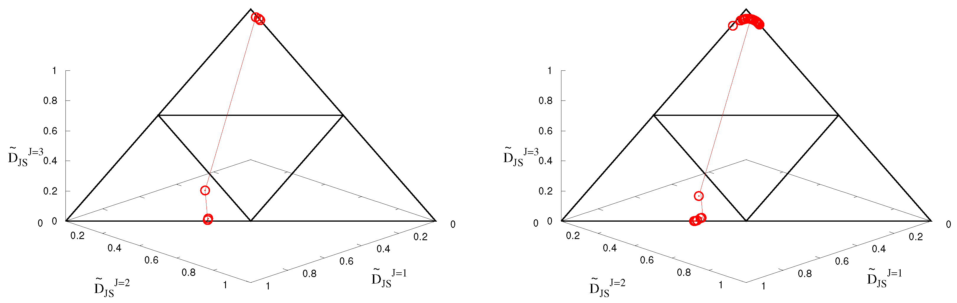
To clearly see the “similarity”, we consider the following normalization; ${\displaystyle {\tilde{D}}_{\mathrm{JS}}^{J=i}=D_{\mathrm{JS}}^{J=i}/\sum _{i=1}^3{D}_{\mathrm{JS}}^{J=i}}$ with $i=1,2,3$. Thus, we can consider 2-simplex which vertexes are ($D_{\mathrm{JS}}^{J=1}$,$D_{\mathrm{JS}}^{J=2}$,$D_{\mathrm{JS}}^{J=3})=(0,1,1),(1,0,1),(0,0,1)$ and then we can trace the ${\tilde{D}}_{\mathrm{JS}}^J$ trajectory on the simplex. The opposite triangle is added as an eye guide in the figure. The right and left panels of Figure 2 show the trajectory on the simplex for lattice data and PNJL model results, respectively.

Data points appearing near the bottom edge are corresponding to the results in the high temperature phase and the data points appearing near the top vertex are the results in the low temperature phase. In both cases, data are well separated; data for low and high T appear around the top vertex and the center of the bottom edge of the 2-simplex, respectively. It indicates that the PNJL model can well reproduce the oscillating modes in lattice QCD data. Then, we can understand the importance of the RW periodicity and also the transition to understand the confinement–deconfinement phenomena. Therefore, the PNJL model can be considered good element assembly to construct the reliable QCD effective model due to the oscillating modes, which directly affect the reliability of the model at finite real chemical potential, existing in the model. Actually, if theory or effective models do not have such oscillating modes, we cannot discuss higher-order cumulants, in principle.

7. Conclusions

In this review, we overview QCD properties at finite imaginary chemical potential and its applications to exploring the QCD phase diagram at a finite real chemical potential. In particular, we explain why the Polyakov-loop extended Nambu–Jona–Lasinio (PNJL) model can be considered as the promising low-energy effective model of QCD.

First, we have explained several important and interesting features of QCD at finite imaginary chemical potential such as the Roberge–Weiss (RW) periodicity and the RW transition based on Ref. [25]. The RW periodicity explains the model independently. In comparison, we employ the strong coupling limit of QCD and the perturbative one-loop effective potential to explain the RW transition. The origin of the RW periodicity is different in the low and high temperature phases; this difference induces the first-order RW transition where the phase of the Polyakov loop and the quark number density have the gap. To understand the RW transition, the spontaneous shift symmetry braking plays a crucial role and then the modified Polyakov-loop is treated as the order-parameter of the symmetry breaking.

In Section 3, it is shown that there is a possibility that we can approach the confinement–deconfinement nature based on several non-trivial interpretations of the imaginary chemical potential such as the temporal fermion boundary angle and the Aharonov–Bohm phase. Based on the interpretations, we have explained why the dual quark-condensate and the quark number holonomy can be considered as the (quantum) order parameter or the indicator of the confinement–deconfinement transition. In addition, we have shown the strategy of the imaginary chemical potential matching approach which combines the low-energy effective model of QCD and the lattice QCD data at finite imaginary chemical potential.

The possible low-energy QCD effective model which can be used in the imaginary chemical potential region has been discussed in Section 4. We have explained why the simple Nambu–Jona–Lasinio (NJL) model can not reproduce the RW periodicity, while the Polyakov-loop extended Nambu–Jona–Lasinio (PNJL) model can. Because of this fact, the PNJL model is the promising low-energy effective model of QCD. Some theoretical problems and confusing points of the PNJL model are also explained. For example, the reason why the model Polyakov-loop cannot be matched with the correct Polyakov-loop is shown. In addition, the detailed reason why the PNJL model has the RW periodicity is explained from the viewpoint of the modified Polyakov-loop; the Fermi–Dirac distribution function of the PNJL model can be expressed by using the modified Polyakov-loop.

In Section 5, we have summarized some approaches to attack the QCD phase diagram at finite real chemical potential via the imaginary chemical potential region; the analytic continuation method, the canonical ensemble method and Lee–Yang zero analysis are explained. Particularly, we show a detailed discussion on the Polyakov-loop paradox appearing in the canonical ensemble method which is important to ensure the foundation of the method. Then, we can see that the usefulness of the modified Polyakov-loop and also the removal of the nontrivial ${\mathbb{Z}}_3$-images from the the canonical ensemble.

Finally, the similarity measure has been discussed to see how the PNJL model and the lattice QCD simulation provide the similar oscillating behavior at finite imaginary chemical potential. Actually, we employ the Jensen–Shannon divergence to measure the similarity. From the results, we can understand that the PNJL model can be used as a promising prime-field to model the QCD properties.

References

- De Forcrand, P. Simulating QCD at finite density. PoS 2009, LAT2009, 010. [Google Scholar]
- Parisi, G.; Wu, Y.S. Perturbation Theory Without Gauge Fixing. Sci. Sin. 1981, 24, 483. [Google Scholar]
- Parisi, G. On complex probabilities. Phys. Lett. 1983, B131, 393–395. [Google Scholar] [CrossRef]
- Witten, E. Analytic Continuation Of Chern-Simons Theory. AMS/IP Stud. Adv. Math. 2011, 50, 347–446. [Google Scholar]
- Cristoforetti, M.; Di Renzo, F.; Scorzato, L. New approach to the sign problem in quantum field theories: High density QCD on a Lefschetz thimble. Phys. Rev. 2012, D86, 074506. [Google Scholar] [CrossRef]
- Fujii, H.; Honda, D.; Kato, M.; Kikukawa, Y.; Komatsu, S.; Sano, T. Hybrid Monte Carlo on Lefschetz thimbles—A study of the residual sign problem. JHEP 2013, 1310, 147. [Google Scholar] [CrossRef]
- Mori, Y.; Kashiwa, K.; Ohnishi, A. Toward solving the sign problem with path optimization method. Phys. Rev. 2017, D96, 111501. [Google Scholar] [CrossRef]
- Mori, Y.; Kashiwa, K.; Ohnishi, A. Application of a neural network to the sign problem via the path optimization method. PTEP 2018, 2018, 023B04. [Google Scholar] [CrossRef]
- Fukushima, K. Chiral effective model with the Polyakov loop. Phys. Lett. 2004, B591, 277–284. [Google Scholar] [CrossRef]
- Haas, L.M.; Braun, J.; Pawlowski, J.M. On the QCD phase diagram at finite chemical potential. AIP Conf. Proc. 2011, 1343, 459–461. [Google Scholar] [CrossRef]
- Biernat, E.P.; Gross, F.; Peña, T.; Stadler, A. Confinement, quark mass functions, and spontaneous chiral symmetry breaking in Minkowski space. Phys. Rev. 2014, D89, 016005. [Google Scholar] [CrossRef]
- Fischer, C.S. QCD at finite temperature and chemical potential from Dyson–Schwinger equations. Prog. Part. Nucl. Phys. 2019, 105, 1–60. [Google Scholar] [CrossRef]
- Biernat, E.P.; Gross, F.; Peña, M.T.; Stadler, A.; Leitão, S. Quark mass function from a one-gluon-exchange-type interaction in Minkowski space. Phys. Rev. 2018, D98, 114033. [Google Scholar] [CrossRef]
- Miyahara, A.; Torigoe, Y.; Kouno, H.; Yahiro, M. Equation of state and transition temperatures in the quark-hadron hybrid model. Phys. Rev. 2016, D94, 016003. [Google Scholar] [CrossRef]
- Gasser, J.; Leutwyler, H. Light Quarks at Low Temperatures. Phys. Lett. 1987, B184, 83–88. [Google Scholar] [CrossRef]
- Allton, C.; Doring, M.; Ejiri, S.; Hands, S.; Kaczmarek, O.; Karsch, F.; Laermann, E.; Redlich, K. Thermodynamics of two flavor QCD to sixth order in quark chemical potential. Phys. Rev. 2005, D71, 054508. [Google Scholar] [CrossRef]
- Borsanyi, S.; Fodor, Z.; Hoelbling, C.; Katz, S.D.; Krieg, S.; Ratti, C.; Szabo, K.K. Is there still any Tc mystery in lattice QCD? Results with physical masses in the continuum limit III. JHEP 2010, 9, 073. [Google Scholar] [CrossRef]
- Borsanyi, S.; Fodor, Z.; Katz, S.D.; Krieg, S.; Ratti, C.; Szabo, K. Fluctuations of conserved charges at finite temperature from lattice QCD. JHEP 2012, 01, 138. [Google Scholar] [CrossRef]
- Borsanyi, S.; Endrodi, G.; Fodor, Z.; Katz, S.D.; Krieg, S.; Ratti, C.; Szabo, K.K. QCD equation of state at nonzero chemical potential: Continuum results with physical quark masses at order mu2. JHEP 2012, 8, 053. [Google Scholar] [CrossRef]
- Hasenfratz, A.; Toussaint, D. Canonical ensembles and nonzero density quantum chromodynamics. Nucl. Phys. 1992, B371, 539–549. [Google Scholar] [CrossRef]
- Alexandru, A.; Faber, M.; Horvath, I.; Liu, K.F. Lattice QCD at finite density via a new canonical approach. Phys. Rev. 2005, D72, 114513. [Google Scholar] [CrossRef]
- Kratochvila, S.; de Forcrand, P. QCD at zero baryon density and the Polyakov loop paradox. Phys. Rev. 2006, D73, 114512. [Google Scholar] [CrossRef]
- De Forcrand, P.; Kratochvila, S. Finite density QCD with a canonical approach. Nucl. Phys. Proc. Suppl. 2006, 153, 62–67. [Google Scholar] [CrossRef] [Green Version]
- Li, A.; Alexandru, A.; Liu, K.F.; Meng, X. Finite density phase transition of QCD with Nf = 4 and Nf = 2 using canonical ensemble method. Phys. Rev. 2010, D82, 054502. [Google Scholar] [CrossRef]
- Roberge, A.; Weiss, N. Gauge Theories With Imaginary Chemical Potential and the Phases of QCD. Nucl. Phys. 1986, B275, 734. [Google Scholar] [CrossRef]
- Sato, M. Topological discrete algebra, ground state degeneracy, and quark confinement in QCD. Phys. Rev. 2008, D77, 045013. [Google Scholar] [CrossRef]
- Wen, X.G. Topological Order in Rigid States. Int. J. Mod. Phys. 1990, B4, 239. [Google Scholar] [CrossRef]
- Kashiwa, K.; Ohnishi, A. Topological feature and phase structure of QCD at complex chemical potential. Phys. Lett. 2015, B750, 282–286. [Google Scholar] [CrossRef]
- Kashiwa, K.; Ohnishi, A. Quark number holonomy and confinement-deconfinement transition. Phys. Rev. 2016, D93, 116002. [Google Scholar] [CrossRef]
- Kashiwa, K.; Ohnishi, A. Topological deconfinement transition in QCD at finite isospin density. Phys. Lett. 2017, B772, 669–674. [Google Scholar] [CrossRef]
- D’Elia, M.; Lombardo, M.P. Finite density QCD via imaginary chemical potential. Phys. Rev. 2003, D67, 014505. [Google Scholar] [CrossRef]
- De Forcrand, P.; Philipsen, O. The QCD phase diagram for small densities from imaginary chemical potential. Nucl. Phys. 2002, B642, 290–306. [Google Scholar] [CrossRef]
- De Forcrand, P.; Philipsen, O. The QCD phase diagram for three degenerate flavors and small baryon density. Nucl. Phys. 2003, B673, 170–186. [Google Scholar] [CrossRef]
- D’Elia, M.; Lombardo, M.P. QCD thermodynamics from an imaginary mu(B): Results on the four flavor lattice model. Phys. Rev. 2004, D70, 074509. [Google Scholar] [CrossRef]
- Chen, H.S.; Luo, X.Q. Phase diagram of QCD at finite temperature and chemical potential from lattice simulations with dynamical Wilson quarks. Phys. Rev. 2005, D72, 034504. [Google Scholar] [CrossRef]
- Bonati, C.; Cossu, G.; D’Elia, M.; Sanfilippo, F. The Roberge-Weiss endpoint in Nf = 2 QCD. Phys. Rev. 2011, D83, 054505. [Google Scholar] [CrossRef]
- Nagata, K.; Nakamura, A. Imaginary Chemical Potential Approach for the Pseudo-Critical Line in the QCD Phase Diagram with Clover-Improved Wilson Fermions. Phys. Rev. 2011, D83, 114507. [Google Scholar] [CrossRef]
- Bonati, C.; de Forcrand, P.; D’Elia, M.; Philipsen, O.; Sanfilippo, F. Chiral phase transition in two-flavor QCD from an imaginary chemical potential. Phys. Rev. 2014, D90, 074030. [Google Scholar] [CrossRef]
- Takahashi, J.; Kouno, H.; Yahiro, M. Quark number densities at imaginary chemical potential in Nf = 2 lattice QCD with Wilson fermions and its model analyses. Phys. Rev. 2015, D91, 014501. [Google Scholar] [CrossRef]
- Doi, T.M.; Kashiwa, K. Dirac-mode expansion of quark number density and its implications of the confinement-deconfinement transition. arXiv 2017, arXiv:1706.00614. [Google Scholar]
- Kashiwa, K.; Sasaki, T.; Kouno, H.; Yahiro, M. Two-color QCD at imaginary chemical potential and its impact on real chemical potential. Phys. Rev. 2013, D87, 016015. [Google Scholar] [CrossRef]
- Sakai, Y.; Kashiwa, K.; Kouno, H.; Yahiro, M. Polyakov loop extended NJL model with imaginary chemical potential. Phys. Rev. 2008, D77, 051901. [Google Scholar] [CrossRef]
- Nishida, Y. Phase structures of strong coupling lattice QCD with finite baryon and isospin density. Phys. Rev. 2004, D69, 094501. [Google Scholar] [CrossRef]
- Kawamoto, N.; Miura, K.; Ohnishi, A.; Ohnuma, T. Phase diagram at finite temperature and quark density in the strong coupling limit of lattice QCD for color SU(3). Phys. Rev. 2007, D75, 014502. [Google Scholar] [CrossRef]
- Garcia Martin, R.; Pelaez, J. Chiral condensate thermal evolution at finite baryon chemical potential within Chiral Perturbation Theory. Phys. Rev. 2006, D74, 096003. [Google Scholar] [CrossRef]
- Ayala, A.; Bashir, A.; Dominguez, C.; Gutierrez, E.; Loewe, M.; Raya, A. QCD phase diagram from finite energy sum rules. Phys. Rev. 2011, D84, 056004. [Google Scholar] [CrossRef]
- Gross, D.J.; Pisarski, R.D.; Yaffe, L.G. QCD and Instantons at Finite Temperature. Rev. Mod. Phys. 1981, 53, 43. [Google Scholar] [CrossRef]
- Weiss, N. The Effective Potential for the Order Parameter of Gauge Theories at Finite Temperature. Phys. Rev. 1981, D24, 475. [Google Scholar] [CrossRef]
- Sakamoto, M.; Takenaga, K. On Gauge Symmetry Breaking via Euclidean Time Component of Gauge Fields. Phys. Rev. 2007, D76, 085016. [Google Scholar] [CrossRef]
- Kouno, H.; Sakai, Y.; Kashiwa, K.; Yahiro, M. Roberge-Weiss phase transition and its endpoint. J. Phys. 2009, G36, 115010. [Google Scholar] [CrossRef]
- Kashiwa, K.; Yahiro, M.; Kouno, H.; Matsuzaki, M.; Sakai, Y. Correlations among discontinuities in the QCD phase diagram. J. Phys. 2009, G36, 105001. [Google Scholar] [CrossRef]
- De Forcrand, P.; Philipsen, O. Constraining the QCD phase diagram by tricritical lines at imaginary chemical potential. Phys. Rev. Lett. 2010, 105, 152001. [Google Scholar] [CrossRef] [PubMed]
- D’Elia, M.; Sanfilippo, F. The Order of the Roberge-Weiss endpoint (finite size transition) in QCD. Phys. Rev. 2009, D80, 111501. [Google Scholar] [CrossRef]
- Bonati, C.; D’Elia, M.; Mariti, M.; Mesiti, M.; Negro, F.; Sanfilippo, F. Roberge-Weiss endpoint at the physical point of Nf = 2 + 1 QCD. Phys. Rev. 2016, D93, 074504. [Google Scholar] [CrossRef]
- Bonati, C.; Calore, E.; D’Elia, M.; Mesiti, M.; Negro, F.; Sanfilippo, F.; Schifano, S.F.; Silvi, G.; Tripiccione, R. Roberge-Weiss endpoint and chiral symmetry restoration in Nf = 2 + 1 QCD. Phys. Rev. 2019, D99, 014502. [Google Scholar] [CrossRef]
- Goswami, J.; Karsch, F.; Lahiri, A.; Schmidt, C. QCD phase diagram for finite imaginary chemical potential with HISQ fermions. arXiv 2018, arXiv:1811.02494. [Google Scholar]
- Shimizu, H.; Yonekura, K. Anomaly constraints on deconfinement and chiral phase transition. Phys. Rev. 2018, D97, 105011. [Google Scholar] [CrossRef]
- Kikuchi, Y. ’t Hooft Anomaly, Global Inconsistency, and Some of Their Applications. Ph.D. Thesis, Kyoto University, Kyoto, Japan, 2018. [Google Scholar]
- Nishimura, H.; Tanizaki, Y. High-temperature domain walls of QCD with imaginary chemical potentials. arXiv 2019, arXiv:1903.04014. [Google Scholar]
- Kashiwa, K.; Matsuzaki, M.; Kouno, H.; Sakai, Y.; Yahiro, M. Meson mass at real and imaginary chemical potentials. Phys. Rev. 2009, D79, 076008. [Google Scholar] [CrossRef]
- Bilgici, E.; Bruckmann, F.; Gattringer, C.; Hagen, C. Dual quark condensate and dressed Polyakov loops. Phys. Rev. 2008, D77, 094007. [Google Scholar] [CrossRef]
- Bilgici, E.; Bruckmann, F.; Danzer, J.; Gattringer, C.; Hagen, C.; Ilgenfritz, E.M.; Maas, A. Fermionic boundary conditions and the finite temperature transition of QCD. Few Body Syst. 2010, 47, 125–135. [Google Scholar] [CrossRef]
- Bilgici, E. Signatures of Confinement and Chiral Symmetry Breaking In Spectral Quantities of Lattice Dirac Operators. Ph.D. Thesis, University of Graz, Graz, Austria, 2009. [Google Scholar]
- Bruckmann, F.; Endrodi, G. Dressed Wilson loops as dual condensates in response to magnetic and electric fields. Phys. Rev. 2011, D84, 074506. [Google Scholar] [CrossRef]
- Fischer, C.S. Deconfinement phase transition and the quark condensate. Phys. Rev. Lett. 2009, 103, 052003. [Google Scholar] [CrossRef]
- Fischer, C.S.; Mueller, J.A. Chiral and deconfinement transition from Dyson-Schwinger equations. Phys. Rev. 2009, D80, 074029. [Google Scholar] [CrossRef]
- Kashiwa, K.; Kouno, H.; Yahiro, M. Dual quark condensate in the Polyakov-loop extended NJL model. Phys. Rev. 2009, D80, 117901. [Google Scholar] [CrossRef]
- Gatto, R.; Ruggieri, M. Dressed Polyakov loop and phase diagram of hot quark matter under magnetic field. Phys. Rev. 2010, D82, 054027. [Google Scholar] [CrossRef]
- Zhang, Z.; Miao, Q. Dual condensates at finite isospin chemical potential. Phys. Lett. B 2015, 753, 670–676. [Google Scholar] [CrossRef]
- Zhang, Z.; Lu, H. Dual meson condensates in the Polyakov-loop extended linear sigma model. arXiv 2017, arXiv:1705.09953. [Google Scholar]
- Xu, F.; Mao, H.; Mukherjee, T.K.; Huang, M. Dressed Polyakov loop and flavor dependent phase transitions. Phys. Rev. 2011, D84, 074009. [Google Scholar] [CrossRef]
- Sasagawa, S.; Tanaka, H. The separation of the chiral and deconfinement phase transitions in the curved space-time. Prog. Theor. Phys. 2012, 128, 925–939. [Google Scholar] [CrossRef]
- Flachi, A. Deconfinement transition and Black Holes. Phys. Rev. 2013, D88, 041501. [Google Scholar] [CrossRef]
- Benič, S. Physical interpretation of the dressed Polyakov loop in the Nambu-Jona-Lasinio model. Phys. Rev. 2013, D88, 077501. [Google Scholar] [CrossRef]
- Aharonov, Y.; Bohm, D. Significance of electromagnetic potentials in the quantum theory. Phys. Rev. 1959, 115, 485–491. [Google Scholar] [CrossRef]
- Huang, S.; Schreiber, B. Statistical mechanics of relativistic anyon-like systems. Nucl. Phys. B 1994, 426, 644–660. [Google Scholar] [CrossRef]
- Kondo, K.I. Toward a first-principle derivation of confinement and chiral-symmetry-breaking crossover transitions in QCD. Phys. Rev. 2010, D82, 065024. [Google Scholar] [CrossRef]
- Kashiwa, K.; Hell, T.; Weise, W. Nonlocal Polyakov-Nambu-Jona-Lasinio model and imaginary chemical potential. Phys. Rev. 2011, D84, 056010. [Google Scholar] [CrossRef]
- Kitazawa, M.; Koide, T.; Kunihiro, T.; Nemoto, Y. Chiral and color superconducting phase transitions with vector interaction in a simple model. Prog. Theor. Phys. 2002, 108, 929–951. [Google Scholar] [CrossRef]
- Kashiwa, K.; Kouno, H.; Sakaguchi, T.; Matsuzaki, M.; Yahiro, M. Chiral phase transition in an extended NJL model with higher-order multi-quark interactions. Phys. Lett. 2007, B647, 446–451. [Google Scholar] [CrossRef]
- Kashiwa, K.; Kouno, H.; Matsuzaki, M.; Yahiro, M. Critical endpoint in the Polyakov-loop extended NJL model. Phys. Lett. 2008, B662, 26–32. [Google Scholar] [CrossRef]
- Sugano, J.; Takahashi, J.; Ishii, M.; Kouno, H.; Yahiro, M. Determination of the strength of the vector-type four-quark interaction in the entanglement Polyakov-loop extended Nambu-Jona-Lasinio model. Phys. Rev. 2014, D90, 037901. [Google Scholar] [CrossRef]
- Braun, J.; Gies, H.; Pawlowski, J.M. Quark Confinement from Color Confinement. Phys. Lett. 2010, B684, 262–267. [Google Scholar] [CrossRef]
- Roessner, S.; Ratti, C.; Weise, W. Polyakov loop, diquarks and the two-flavour phase diagram. Phys. Rev. 2007, D75, 034007. [Google Scholar] [CrossRef]
- Schaefer, B.J.; Pawlowski, J.M.; Wambach, J. The Phase Structure of the Polyakov—Quark-Meson Model. Phys. Rev. 2007, D76, 074023. [Google Scholar] [CrossRef]
- Haas, L.M.; Stiele, R.; Braun, J.; Pawlowski, J.M.; Schaffner-Bielich, J. Improved Polyakov-loop potential for effective models from functional calculations. Phys. Rev. 2013, D87, 076004. [Google Scholar] [CrossRef]
- Meisinger, P.N.; Miller, T.R.; Ogilvie, M.C. Phenomenological equations of state for the quark gluon plasma. Phys. Rev. 2002, D65, 034009. [Google Scholar] [CrossRef]
- Pisarski, R.D. Why the quark gluon plasma isn’t a plasma. In Proceedings of the Strong and Electroweak Matter Meeting (SEWM), Marseille, France, 13–17 June 2000; pp. 107–117. [Google Scholar] [CrossRef]
- Dumitru, A.; Pisarski, R.D. Degrees of freedom and the deconfining phase transition. Phys. Lett. 2002, B525, 95–100. [Google Scholar] [CrossRef]
- Scavenius, O.; Dumitru, A.; Lenaghan, J.T. The K/pi ratio from condensed Polyakov loops. Phys. Rev. 2002, C66, 034903. [Google Scholar] [CrossRef]
- Ratti, C.; Thaler, M.A.; Weise, W. Phases of QCD: Lattice thermodynamics and a field theoretical model. Phys. Rev. 2006, D73, 014019. [Google Scholar] [CrossRef]
- Dumitru, A.; Guo, Y.; Hidaka, Y.; Altes, C.P.K.; Pisarski, R.D. How Wide is the Transition to Deconfinement? Phys. Rev. 2011, D83, 034022. [Google Scholar] [CrossRef]
- Fukushima, K.; Kashiwa, K. Polyakov loop and QCD thermodynamics from the gluon and ghost propagators. Phys. Lett. 2013, B723, 360–364. [Google Scholar] [CrossRef]
- Kashiwa, K.; Pisarski, R.D.; Skokov, V.V. Critical endpoint for deconfinement in matrix and other effective models. Phys. Rev. 2012, D85, 114029. [Google Scholar] [CrossRef]
- Kashiwa, K.; Pisarski, R.D. Roberge-Weiss transition and ’t Hooft loops. Phys. Rev. 2013, D87, 096009. [Google Scholar] [CrossRef]
- Bornyakov, V.G.; Boyda, D.L.; Goy, V.A.; Molochkov, A.V.; Nakamura, A.; Nikolaev, A.A.; Zakharov, V.I. New approach to canonical partition functions computation in Nf = 2 lattice QCD at finite baryon density. Phys. Rev. 2017, D95, 094506. [Google Scholar] [CrossRef]
- Karbstein, F.; Thies, M. How to get from imaginary to real chemical potential. Phys. Rev. D 2007, 75, 025003. [Google Scholar] [CrossRef]
- Kouji, K.; Hiroaki, K. Roberge-Weiss periodicity, canonical sector and modified Polyakov-loop. arXiv 2019, arXiv:1903.11737. [Google Scholar]
- Yang, C.N.; Lee, T.D. Statistical theory of equations of state and phase transitions. 1. Theory of condensation. Phys. Rev. 1952, 87, 404–409. [Google Scholar] [CrossRef]
- Nakamura, A.; Nagata, K. Probing QCD phase structure using baryon multiplicity distribution. PTEP 2016, 2016, 033D01. [Google Scholar] [CrossRef]
- Nagata, K.; Kashiwa, K.; Nakamura, A.; Nishigaki, S.M. Lee-Yang zero distribution of high temperature QCD and the Roberge-Weiss phase transition. Phys. Rev. 2015, D91, 094507. [Google Scholar] [CrossRef]
- Wakayama, M.; Borynakov, V.G.; Boyda, D.L.; Goy, V.A.; Iida, H.; Molochkov, A.V.; Nakamura, A.; Zakharov, V.I. Lee-Yang zeros in lattice QCD for searching phase transition points. arXiv 2018, arXiv:1802.02014. [Google Scholar]
- Kashiwa, K.; Ohnishi, A. Investigation of confinement-deconfinement transition via probability distributions. arXiv 2017, arXiv:1712.06220. [Google Scholar]
- Almasi, G.A.; Friman, B.; Morita, K.; Lo, P.M.; Redlich, K. Fourier coefficients of the net-baryon number density and chiral criticality. arXiv 2018, arXiv:1805.04441. [Google Scholar]
- Ejiri, S.; Karsch, F.; Redlich, K. Hadronic fluctuations at the QCD phase transition. Phys. Lett. 2006, B633, 275–282. [Google Scholar] [CrossRef]
- Karsch, F.; Redlich, K. Probing freeze-out conditions in heavy ion collisions with moments of charge fluctuations. Phys. Lett. 2011, B695, 136–142. [Google Scholar] [CrossRef]
- Lin, J. Divergence measures based on the Shannon entropy. IEEE Trans. Inf. Theory 1991, 37, 145–151. [Google Scholar] [CrossRef] [Green Version]
Figure 1.
The -dependence of and . The dotted and solid lines represent the result at and 300 MeV, respectively.
Figure 2.
The right and left panels show the trajectory on the 2-simplex for the PNJL model and the lattice QCD data [39], respectively.
© 2019 by the author. Licensee MDPI, Basel, Switzerland. This article is an open access article distributed under the terms and conditions of the Creative Commons Attribution (CC BY) license (http://creativecommons.org/licenses/by/4.0/).
Share and Cite
MDPI and ACS Style
Kashiwa, K. Imaginary Chemical Potential, NJL-Type Model and Confinement–Deconfinement Transition. Symmetry 2019, 11, 562. https://doi.org/10.3390/sym11040562
AMA Style
Kashiwa K. Imaginary Chemical Potential, NJL-Type Model and Confinement–Deconfinement Transition. Symmetry. 2019; 11(4):562. https://doi.org/10.3390/sym11040562
Chicago/Turabian StyleKashiwa, Kouji. 2019. "Imaginary Chemical Potential, NJL-Type Model and Confinement–Deconfinement Transition" Symmetry 11, no. 4: 562. https://doi.org/10.3390/sym11040562
Note that from the first issue of 2016, this journal uses article numbers instead of page numbers. See further details here.