Power-Law Distribution of Natural Visibility Graphs from Reaction Times Series


1
Fundación para el Fomento de la Investigación Sanitaria y Biomédica de la Comunitat Valenciana (FISABIO-Public Health), 46020-València, Spain
2
Department of Developmental and Educational Psychology, Universitat de València, 46010-València, Spain
3
Instituto Universitario de Matemática Pura y Aplicada, Universitat Politècnica de València, 46022-València, Spain
*
Author to whom correspondence should be addressed.
Symmetry 2019, 11(4), 563; https://doi.org/10.3390/sym11040563
Submission received: 1 March 2019
/
Revised: 16 April 2019
/
Accepted: 16 April 2019
/
Published: 18 April 2019
(This article belongs to the Special Issue New Trends in Dynamics)
Abstract
:In this study, we analyze the response times of students to yes/no decision tasks from the perspective of network science. We analyze the properties of the natural visibility graphs (NVG) associated with their reaction time series. We observe that the degree distribution of these graphs usually fits a power-law distribution . We study the range in which parameter occurs and the changes of this exponent with respect to the age and gender of the students. In addition to this, we also study the links between the parameter and the parameters of the ex-Gaussian distribution that best fit the response times for each subject.
1. Introduction
1.1. Attention and Reaction Times
Attention is a broad psychological concept, and as a mental construct, it can only be measured indirectly [1] through behaviors such as motor or visual reactions. Attention can be assessed with different instruments: standardized questionnaires, clinical interviews, direct observation of target behaviors, physiological and medical tests, functional magnetic resonance, or through experimental tasks implemented with different software programs, as in references [2,3,4,5,6,7], which is the method used for the present study.
The study of attentional problems is a relevant topic of study in school and clinical settings. Attention deficit/hyperactivity disorder (ADHD) is the most common neurobehavioral disorder in the childhood period. It can profoundly affect the academic performance, well-being, and social interactions of children. The prevalence rate of this disorder is approximately 8% in the normal population [8], and it is higher among children with psychopathological disorders [9]. Further information on attention deficit and hyperactivity disorders can be found in references [10,11,12,13].
In this context, time reaction or response times (RTs) are described as the most accurate measure of perception/attention, decision-making, and other cognitive processes to be considered in clinical and normative settings [14,15,16].
RT recordings (from computerized test batteries developed with the above-mentioned specific software) are an excellent method of assessing attention, including the two main characteristics: speed (measured in milliseconds) and trial/error rate. The analysis of the RT associated with solutions to certain tasks permits us to assess the attention of a subject. It can also help us to find different behavioral pattern differences by age or gender, specifically in visual attention and reaction time of school-aged children [17,18].
1.2. Gender Differences
Differences in ADHD prevalence by sex are well documented. The condition is more frequent in boys than in girls, with ratios that range from 2:1 to 9:1, depending on the subtype and the setting [19,20,21,22]. This is congruent with other studies which have shown that on average males have a higher variance of inattentiveness and hyperactivity/impulsivity than females [23,24].
Furthermore, many previous studies have pointed out gender differences in several psychological domains. A classical meta-analysis was completed by Byrnes, Miller, and Schafer [25] highlighting that several variables, such as biological maturation, self-perceptions, risk perceptions, perceptions of social environment, etc., could explain observed differences of risk taking between genders. More specifically, women may be less effective than men in competitive environments, even if they are able to perform similarly in non-competitive situations [26]. Other authors have studied behaviors in computing tasks [27], pointing out that women shift away from competition while men embrace it. We can see the same gender influence even in scholarly contexts. Girls, either doing poorly or doing well in school, seem to be more vulnerable to internal distress than boys [28]. In this regard, even an objective assessment through an unbiased computing task, as we have applied in this study, could be affected by these gender-related psychological differences.
1.3. Mathematical Distribution of RTs
The RTs usually follow an ex-Gaussian distribution [29,30,31]. The fit of the RTs’ distribution to probabilistic functions is usually performed with the figure of merit of maximizing the likelihood function [32]. Several studies have recently been developed with the goal of setting a correspondence between the three parameters μ, σ, and τ of an ex-Gaussian distribution of RTs derived from performance tests, such as Conners’ continuous performance tests [33], with attention disorders. Of all three parameters, the most interesting one seems to be τ, since it has been assumed to contain a perceptual portion of an RT, the decision component, and it has been recently related to factors associated with attention. For a recent account on the relevance of these three parameters in the diagnosis of ADHD, see references [34,35,36,37,38].
Nevertheless, when fitting to an ex-Gaussian distribution, a loss of information occurs, since the sequential order in which the response times are given by the subject is not considered. Moreover, when the time for responding is exceeded, these items are not usually taken into account in the fit.
1.4. Outline of the Work
In the current study, we followed a radically different approach, closer to time series analysis, in which we also provided a simple graphic interpretation of the results provided by natural visibility graphs (NVGs). From this perspective, a univariate time series was mapped into an abstract graph, with the goal of describing the time series in graph-theoretical terms. NVGs permitted us not only to provide a visual description of a given time series but also to connect the time series itself with the degree distribution of the corresponding graph.
We showed that the NVGs’ degree distributions tended to follow a power-law distribution, in the spirit of free-scale networks (see references [39,40]). We also studied the correlations between the power-law fit parameter and the ex-Gaussian parameters of the distribution [41]. The number of commission errors (when the item was responded to on time with an erroneous answer) and omission errors (when the maximum permitted time was reached and there was no answer provided) were also explored. In addition to this, we analyzed the NVG degree distribution of extreme cases when the number of commission errors were out of the expected range. A brief preliminary description of this approach was presented in reference [42].
2. Materials
A total of 130 students ranging from 8 to 12 years of age located in the Valencia Region, Spain, participated in the study: 66 (50.8%) females and 64 (49.2%) males between 8 and 12 years of age (Table 1). The legal authorization of regional education authorities was obtained to develop this research. All children’s parents/tutors signed the informed consent document allowing their child’s participation. A description of the population can be found in Table 1. The median age was 9 years and the interquartile range was 8–10 years.
The students participating in the study took a lexical decision task test of type yes/no, processed using DMDX software on a laptop [5]. The task consisted of the presentation of a set of letters on the laptop screen. The student had to answer whether a letter P appeared or did not appear. A total of 120 of these stimuli were presented to the student. The maximum time permitted to answer each item was set at 2500 milliseconds (ms). If the student did not answer within the time, then a new stimulus was presented to the student.
In addition, a minimum threshold for considering an admissible reaction time was set at 100 ms, answers under this threshold were discarded since they were considered to be unconscious. This task was inspired by an adaptation of the attention tasks for children presented in reference [43].
3. Methods (Natural Visibility Graph)
The NVGs were introduced by Lacasa et al. [44] and they permitted us to give a visual representation of time series in the plane. This approach has been extensively used in different areas such as economics [45,46], linguistics [47], meteorology [48], and seismology [49,50]. Moreover, NVGs have been successfully applied to diagnose Alzheimer’s disease [51,52] and epilepsy [53], as well as to the classification of sleep stages [54].
We briefly outline how to construct an NVG from a time series. First, we considered the response times sequence . Then, we integrated them as follows: , , where is the jth response time and is the mean value. Following this procedure, the integrated response times were within the fractional Brownian motion regime. In this way, NVGs provided more reliable information on the emerging networks by means of quantities like the degree distribution.
The integrated series of time observations are shown in Figure 1. The associated NVG graph, , where is the set of nodes and is the set of edges, was constructed as follows: We associated to each integrated observation a node . Two nodes were connected by an edge in , if and only if, we could connect the points with a segment without finding any other crossing for that segment or any other one. In Figure 1, we illustrate the construction of the graph from a given time series.
NVGs satisfy nice, interesting properties from the point of view of network science [55]. These graphs are connected, undirected, and invariant under affine transformations of the magnitudes observed in the data series, that is to say, they are invariant under rescaling both the horizontal and vertical axes. The distribution of the number of connections of each node of these graphs is strongly linked with the time series properties. For instance, a periodic series in which some finite pattern of times is repeated is represented by a graph whose nodes have the same degrees (a regular graph). In the same way, random series are represented by random graphs. For a detailed description of these properties refer to references [44,56].
Furthermore, there are striking connections between fractal series, scale-free networks, and self-similar networks. As a matter of fact, a stochastic time series is transformed into a scale-free graph whose degree distributions follow a power-law function, , where . Further information regarding these connections can be found in references [39,57,58,59,60].
4. Results
4.1. Description of the RTs
First, we present a brief description of the RT data. Table 2 shows the results by age and sex.
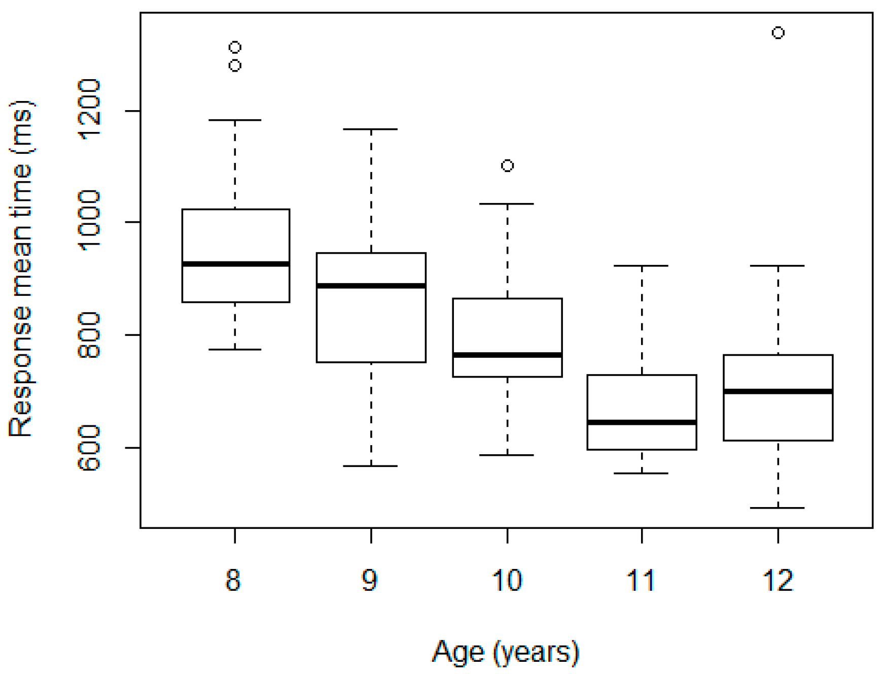
There are no statistically significant differences by sex when exploring the RT means (p-value equal to 0.6226 for the t-test with 95% confidence). The results are presented in Figure 2 and Figure 3. We can see that there are only three and four outliers in each case. These cases will be discussed later in detail.
In contrast, the Kruskal-Wallis test revealed statistically significant differences by age (p-value of 5.27 × 10⁻¹⁰). Specifically, there were differences for ages between 8 and 9 years, 9 and 10 years, and 10 and 11 years, but not between 11 and 12 years, according to the Wilcoxon test. We repeated the test after eliminating the outlier in the 12-year-old group and the result did not vary. These results are consistent with the findings on how reaction times evolve with age [38,61,62,63,64]. A linear model was adjusted taking the logarithm of RT mean as the dependent variable, and age and sex as the fixed-effect factors, obtaining the same results: significant differences across ages 8 and 9 years (10% less RT mean, p-value = 0.01); 9 and 10 years (8% less, p-value = 0.05); 10 and 11 years (15% less, p-value < 0.01); and not between sexes (p-value for sex 0.82).
4.2. Power-Law Distribution of the NVGs’ Degrees
Once we computed the degree distribution of each NVG, we fit each one of these distributions to a power-law, following the procedure described in reference [41]. For this fit, the relevant values are α, the exponent of the power-law, and , the lower bound from which the power-law fit is performed. The use of is necessary since the fitting of empirical data to a power-law is always performed from this value onwards. We estimate this value by , the value that makes it such that for all , the probability distribution of the empirical data and the best-fit power-law model are as close as possible.
In order to compute the distance between these pairs of distributions, we chose the Kolmogorov-Smirnov (K-S) statistic, which is defined as the maximum distance between the two following cumulative distribution functions (CDFs):
- (a)
- , which is the CDF of the empirical data;
- (b)
- , which is the CDF for the power-law fit.
In other words, this distance is computed as . Then, is the value of that minimizes .
For computational purposes, the power-law is considered as where is the Hurwitz zeta function. Then, is computed in order to maximize the likelihood function For specific details, we refer readers to reference [41].
To explore the goodness-of-fit, we generated a large number of power-law-distributed datasets using as α and those values obtained from the distribution that best fits the observed data. Each generated dataset was fitted to a power-law distribution, and the K-S statistic was computed with respect to its own model. Then, we counted for the fraction of time that the K-S statistic was larger than the value of the empirical data. The p-value of the goodness-of-fit was estimated as the fraction of the time that the K-S statistic was larger than that obtained for the observed data. For additional details, we again refer readers to reference [41].
We point out that the p-values should be interpreted with caution, especially if we are dealing with very few data, as larger p-values do not indicate that the power-law is the most appropriate distribution for our data. The correct interpretation is that it is difficult to discard the power-law when we have few data. In our case, we accepted the power-law distribution for 75% of the students. A summary of the values of the parameter α of the power-law can be found in Table 3.
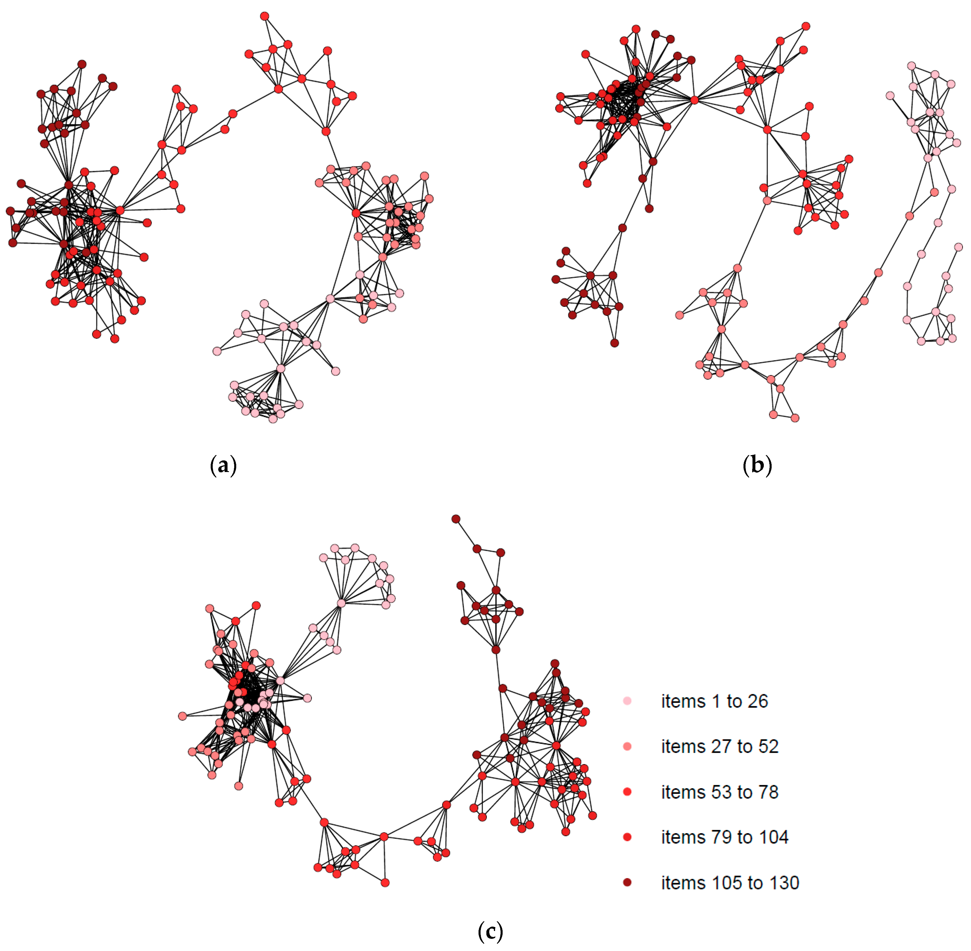
To illustrate the fitting of the degree distribution of NVGs to a power-law distribution, we visualize the NVGs associated with students who did not have omission or commission errors (participants 39, 77, 103) in Figure 4 and Figure 5.
In order to study the NVGs’ complexity, we analyzed the Shannon entropy of the NVGs’ degree distributions. Here, it is defined as the expected value of the information content of the variable, that is, the probability that a node of an NVG has degree . This was initially considered in this setting by Lacasa et al. [65]. More precisely, it is defined as , where is the number of nodes of each graph, and is the probability that the node has degree . The entropy results are summarized in Table 4.
There is no association between the Shannon entropy of the degree distribution and the RT means (Spearman correlation of −0.03). In contrast, there is a strong association between the NVGs’ mean degree and the Shannon entropy (Spearman correlation of 0.991).
It is worth mentioning that when analyzing the NVGs’ mean degree, we did not find any statistically significant differences either by sex (p-value = 0.748 for the Wilcoxon test) or by age (p-value of 0.8022 for the Kruskal-Wallis test). The results are presented in Figure 6 and Figure 7.
Moreover, a linear model including age, sex, and their interaction as predictors and the logarithm of the NVG’s mean degree as response variable was adjusted to corroborate this affirmation. The obtained p-values were 0.530, 0.591, and 0.618 for age, sex, and their interaction, respectively.
4.3. Comparison Between the Power-Law and the Ex-Gaussian Distribution Parameters
Because of the importance of ex-Gaussian distributions in RT analyses, we studied whether there is a relation between NVG complexity and the three parameters that characterize an ex-Gaussian distribution. These parameters represent the mean of the quick responses (), the standard deviation of the quick responses (), and the variability of the slow responses (). It should be noted that there is a strong association between the RT mean and (Spearman correlation of 0.846) and between the RT mean and (Spearman correlation of 0.720). There is also a weaker link between the RT mean and (Spearman correlation of 0.575). The ex-Gaussian parameters for the fitting of the RT frequency distribution were calculated by maximum likelihood as indicated in reference [32]. A summary of the results is presented in Table 5.
The α parameter from the power-law fit and the μ and σ parameters are negatively, not statistically significantly correlated, with Spearman correlation coefficients of −0.062 and −0.042, respectively. However, there was a stronger positive association, although not statistically significant, between α and the τ parameter (0.079).
Returning to the aforementioned cases, the results of students 39, 77, and 103 are representative for what is expected of an RT distribution, since their RTs’ frequencies follow ex-Gaussian distributions in each case (see Figure 8). Despite these participants not committing errors in their answers, they did not need the longest times to respond. Participants 77 and 103 were faster than participant 39 but were older (i.e., 11 years old versus 8 years old).
All parameters, , , , and were positively correlated with the RT mean with correlation coefficients 0.017, 0.768, 0.571, and 0.811, respectively, when response times equal to 2500 ms were not taken into account. However, no association was found when comparing the RT mean with α (Spearman correlation coefficient of 0.017). A linear model was fitted to assess those results obtaining no significant association between the RT mean and α (p-value = 0.140) and between the RT mean and σ (p-value = 0.055).
We found non-remarkable Spearman correlations of the NVG mean degree with (−0.196), (−0.026), (−0.072), and (−0.02). On the other hand, as expected, negative Spearman correlations were also detected between the Shannon entropy and all fitting parameters: (−0.185), (−0.041), (−0.074), and (−0.021).
Finally, three different generalized linear models were adjusted to study the association between , , , and and the number of errors of omission, errors of commission, and hits.
On the one hand, we obtained a significant association between τ and the number of errors of omission. The number of errors of omission increases as long as increases (when increases by 1 unit, omission errors increase 0.7%).
On the other hand, the number of commission errors decreases while μ increases (when μ increases by 1 unit, commission errors decrease 0.2%) and increases while and increase (when σ increases by 1 unit, commission errors increase 0.6%, and when increases by 1 unit, these errors increase 0.3%). These effects remain after adjusting for age and sex. No other significant results were obtained for the other parameters. Finally, the number of hits increases while increases (0.2% more for every increment of by 1 unit), however, the number of hits decreases as and increase (0.5% less when increases by 1 unit, and 0.4% less when increases by 1 unit). All the described effects remain after adjusting the respective models for age and sex.
4.4. Particular Cases
In order to see how each parameter works, we also analyzed in detail the most extreme cases, the parameters of which are presented in Table 6 and Table 7:
Participant 89 was the slowest despite being 12 years old. The and parameters for this participant were the highest among those of all selected participants, and in contrast was the smallest. Participant 120 was the student who committed more errors than the rest. This participant had the lowest value of and the highest of . Finally, participant 84 was the fastest one. The entropy value for this participant was the lowest, as were the and parameters. In the following sections, we compare them graphically. We compare their NVGs, their fit to the power-law of the degree distribution, and their fit to ex-Gaussian distributions in Figure 9, Figure 10, Figure 11 and Figure 12.
5. Discussion and Conclusions
We showed that the degree distribution of the NVG associated with one of these series usually follows a power-law distribution of the form , with . With such an approach, the order in which the items are answered is preserved, in contrast with fitting to an ex-Gaussian distribution of the histogram of the response time frequencies.
Moreover, we also analyzed the correlations between the aforementioned parameter α obtained through a power-law and the ex-Gaussian parameters , , and . We observed that the parameter is weakly negatively correlated with μ and σ and weakly positively correlated with . Stronger correlations were found between the mean response time and the and parameters, and those results were corroborated through a linear model fit. In particular, these connections can be noticed when studying participant 89, the slowest one, with the finding that in this case, the parameter was the highest among the participants. We also see these connections when studying participant 84, the fastest one, with the finding that their parameter was the lowest one. Other potential approaches can be made based on the use of high-order statistical techniques, for example, in references [66,67].
Participants tend to respond faster as age increases from 8 to 11 years, with no differences between sexes as the linear regression revealed. The same pattern is repeated when looking at the standard deviations of the RTs. Males responded faster, but not significantly differently than females, and with higher RT variability. No differences were detected between sex or age when comparing NVGs’ mean degrees.
The number of omission errors increases as increases. The number of commission errors decreases while increases, and it increases while and do. These effects can be seen when studying participant 120, the participant with the largest number of commission errors, the lowest α, and the highest σ. The number of hits increases as increases and decreases while σ and τ increase. In all these cases, the effects are still noticed after considering participants’ age and sex.
An exploratory analysis was performed to detect outliers or influential observations among participants. Before carrying out the complete analysis, we removed two participants from our dataset as they gave no response to almost all items. Finally, we considered 130 participants from 8 to 12 years, however, numbers were reduced when dividing the group by sex and/or age.
Although statistically significant differences were found across age groups, no relevant differences were observed when comparing boys and girls. This fact may be due to the small sample size, which in observational studies such as this one may result in weak statistical significances like those seen here. The obtained results require careful interpretation and should be confirmed with larger sample sizes.
Finally, only one task related to attention was employed to study differences among participants. A wider variety of tasks performed in a larger size sample would provide more robust conclusions. Moreover, such results may be combined in order to provide techniques to dissociate students that may be suffering an attention disorder that should be later clinically confirmed.
Author Contributions
Conceptualization, E.N.-P. and J.A.C.; methodology, J.A.C., A.M.-I., and E.N.-P.; software, A.M.-I., J.A.C.; validation, J.A.C., A.M.-I., and E.N.-P.; formal analysis, A.M.-I. and J.A.C.; investigation, E.N.-P., J.A.C., and A.M.-I.; resources, E.N.-P. and J.A.C.; data curation, E.N.-P.; writing—original draft preparation, A.M.-I.; writing—review and editing, E.N.-P., J.A.C., and A.M.-I.; visualization, J.A.C., A.M.-I., and E.N.-P.; supervision, J.A.C.; project administration, J.A.C.; funding acquisition, J.A.C.
Funding
JAC was partial funded by MEC, grant number 2016-75963-P.
Acknowledgments
The authors acknowledge all the participants and their families.
Conflicts of Interest
The authors declare no conflict of interest.
References
- Spikman, J.; Zomeren, E.V. The Handbook of Clinical Neuropsychology; Gurd, J., Kischka, U., Marshal, J., Eds.; Oxford University Press: Oxford, UK, 2010; pp. 81–96. [Google Scholar]
- Hart, H.; Radua, J.; Nakao, T.; Mataix-Cols, D.; Rubia, K. Meta-analysis of functional magnetic resonance imaging studies of inhibition and attention in attention-deficit/hyperactivity disorder: Exploring task-specific, stimulant medication, and age effects. JAMA Psychiatr. 2013, 70, 185–198. [Google Scholar] [CrossRef]
- Ponsford, J.; Kinsella, G. The use of a rating scale of attentional behavior. Neuropsychol. Rehabil. 1991, 1, 241–257. [Google Scholar] [CrossRef]
- Conners, C.K.; Staff, M.H.S.; Connelly, V.; Campbell, S.; MacLean, M.; Barnes, J. Conners’ continuous performance Test II (CPT II v. 5). Multi-Health Syst. Inc. 2000, 29, 175–196. [Google Scholar]
- Forster, K.I.; Forster, J.C. DMDX: A Windows display program with millisecond accuracy. Behav. Res. Methods Instrum. Comput. 2003, 35, 116–124. [Google Scholar] [CrossRef]
- Mathôt, S.; Schreij, D.; Theeuwes, J. OpenSesame: An open-source, graphical experiment builder for the social sciences. Behav. Res. Methods 2012, 44, 314–324. [Google Scholar] [CrossRef]
- Spapé, M.; Verdonschot, R.; Dantzig, S.V.; Steenbergen, H.V. The E-Primer: An Introduction to Creating Psychological Experiments in E-Prime®; Leiden University Press: Leiden, The Netherlands, 2014; Volume 208. [Google Scholar]
- Subcommittee on Attention-Deficit/Hyperactivity Disorder, Steering committee on Quality Improvement and Management. ADHD: Clinical practice guideline for the diagnosis, evaluation, and treatment of attention-deficit/hyperactivity disorder in children and adolescents. Pediatrics 2011, 128, 2011–2654. [Google Scholar]
- Boyle, C.A.; Boulet, S.; Schieve, L.A.; Cohen, R.A.; Blumberg, S.J.; Yeargin-Allsopp, M.; Visser, S.; Kogan, M.D. Trends in the prevalence of developmental disabilities in US children, 1997–2008. Pediatrics 2011, 127, 1034–1042. [Google Scholar] [CrossRef]
- Barkley, R.A. (Ed.) Attention-Deficit Hyperactivity Disorder: A Handbook for Diagnosis and Treatment; Guilford Publications: New York, NY, USA, 2014. [Google Scholar]
- Thomas, R.; Sanders, S.; Doust, J.; Beller, E.; Glasziou, P. Prevalence of attention-deficit/hyperactivity disorder: A systematic review and meta-analysis. Pediatrics 2015, 135, e994–e1001. [Google Scholar] [CrossRef] [PubMed]
- Willcutt, E.G.; Nigg, J.T.; Pennington, B.F.; Solanto, M.V.; Rohde, L.A.; Tannock, R.; Loo, S.K.; Carlson, C.L.; McBurnett, K.; Lahey, B.B. Validity of DSM-IV attention deficit/hyperactivity disorder symptom dimensions and subtypes. J. Abnorm. Psychol. 2012, 121, 991. [Google Scholar] [CrossRef]
- Visser, S.N.; Danielson, M.L.; Bitsko, R.H.; Holbrook, J.R.; Kogan, M.D.; Ghandour, R.M.; Perou, R.; Blumberg, S.J. Trends in the parent-report of health care provider-diagnosed and medicated attention-deficit/hyperactivity disorder: United States, 2003–2011. J. Am. Acad. Child Adolesc. Psychiatry 2014, 53, 34–46. [Google Scholar] [CrossRef] [PubMed]
- Merritt, P.; Hirshman, E.; Wharton, W.; Stangl, B.; Devlin, J.; Lenz, A. Evidence for gender differences in visual selective attention. Pers. Individ. Differ. 2007, 43, 597–609. [Google Scholar] [CrossRef]
- Dye, M.W.G.; Bavelier, D. Differential development of visual attention skills in school-age children. Vision Res. 2010, 50, 452–459. [Google Scholar] [CrossRef]
- Vaquero, E.; Cardoso, M.J.; Vázquez, M.; Gómez, C.M. Gender differences in event-related potentials during visual-spatial attention. Int. J. Neurosci. 2004, 114, 541–557. [Google Scholar] [CrossRef]
- Halperin, J.M.; Wolf, L.E.; Pascualvaca, D.M.; Newcorn, J.H.; Healey, J.M.; O’BRIEN, J.D.; Morganstein, A.; Young, J.G. Differential assessment of attention and impulsivity in children. J. Am. Acad. Child Adolesc. Psychiatry 1988, 27, 326–329. [Google Scholar] [CrossRef]
- Schatz, A.M.; Ballantyne, A.M.; Trauner, D.A. Sensitivity and specificity of a computerized test of Attention in the diagnosis of Attention-Deficit/Hyperactivity Disorder. Assesment 2001, 8, 357–365. [Google Scholar] [CrossRef]
- Rucklidge, J.J. Gender differences in attention-deficit/hyperactivity disorder. Psychiatr. Clin. 2010, 33, 357–373. [Google Scholar] [CrossRef]
- Faraone, S.V.; Asherson, P.; Banaschewski, T.; Biederman, J. Attention-deficit/hyperactivity disorder. Nat. Rev. Dis. Primers 2015, 1, 15020. [Google Scholar] [CrossRef]
- Polanczyk, G.; de Lima, M.S.; Horta, B.L.; Biederman, J.; Rohde, L.A. The worldwide prevalence of ADHD: A systematic review and metaregression analysis. Am. J. Psychiatry 2007, 164, 942–948. [Google Scholar] [CrossRef]
- Gaub, M.; Carlson, C.L. Gender differences in ADHD: A meta-analysis and critical review. J. Am. Acad. Child Adolesc. Psychiatry 1997, 36, 1036–1045. [Google Scholar] [CrossRef]
- Gershon, J. Meta-analysis gender differences ADHD. J. Atten. Disord. 2002, 5, 143–154. [Google Scholar] [CrossRef]
- Arnett, A.B.; Pennington, B.F.; Willcutt, E.G.; DeFries, J.C.; Olson, R.K. Sex differences in ADHD symptom severity. J. Child Psychol. Psychiatry 2015, 56, 632–639. [Google Scholar] [CrossRef] [PubMed]
- Byrnes, J.P.; Miller, D.C.; Schafer, W.D. Gender differences in risk taking: A meta-analysis. Psychol. Bull. 1999, 125, 367–383. [Google Scholar] [CrossRef]
- Gneezy, U.; Niederle, M.; Rustichini, A. Performance in competitive environments: Gender differences. Q. J. Econ. 2003, 118, 1049–1074. [Google Scholar] [CrossRef]
- Niederle, M.; Vesterlund, L. Do women shy away from competition? Do men compete too much? Q. J. Econ. 2007, 122, 1067–1102. [Google Scholar] [CrossRef]
- Pomerantz, E.M.; Altermatt, E.R.; Saxon, J.L. Making the grade but feeling distressed: Gender differences in academic performance and internal distress. J. Educ. Psychol. 2002, 94, 396–404. [Google Scholar] [CrossRef]
- Balota, D.A.; Melvin, J.Y. Moving beyond the mean in studies of mental chronometry: The power of response time distributional analyses. Curr. Dir. Psychol. Sci. 2011, 20, 160–166. [Google Scholar] [CrossRef]
- Luce, R.D. Response Times: Their Role in Inferring Elementary Mental Organization; Oxford University Press: Oxford, UK, 1986. [Google Scholar]
- Ratcliff, R.; Murdock, B.B. Retrieval processes in recognition memory. Psychol. Rev. 1976, 83, 190–214. [Google Scholar] [CrossRef]
- Lacouture, Y.; Coisenau, D. How to use MATLAB to fit the ex-Gaussian and other probability functions to a distribution of response times. Tutor. Quant. Methods Psychol. 2008, 4, 35–45. [Google Scholar] [CrossRef]
- Conners, C.K.; Epstein, J.N.; Angold, A.; Klaric, J. Continuous performance test performance in a normative epidemiological sample. J. Abnorm. Child Psychol. 2003, 31, 555–562. [Google Scholar] [CrossRef]
- Buzy, W.M.; Medoff, D.R.; Schweitzer, J.B. Intra-individual variability among children with ADHD on a working memory task: An ex-Gaussian approach. Child Neuropsychol. 2009, 15, 441–459. [Google Scholar] [CrossRef]
- Gmehlin, D.; Fuermaier, A.B.; Walther, S.; Debelak, R.; Rentrop, M.; Westermann, C.; Sharma, A.; Tucha, L.; Koerts, J.; Tucha, O.; et al. Intraindividual variability in inhibitory function in adults with ADHD—An ex-Gaussian approach. PLoS ONE 2014, 9, e112298. [Google Scholar] [CrossRef] [PubMed]
- Gu, S.H.; Gau, S.S.; Tzang, S.; Hsu, W. The ex-Gaussian distribution of reaction times in adolescents with attention-deficit/hyperactivity disorder. Res. Dev. Disabil. 2013, 34, 3709–3719. [Google Scholar] [PubMed]
- Moret-Tatay, C.; Leth-Steensen, C.; Irigaray, T.Q.; Argimon, I.I.; Gamermann, D.; Abad-Tortosa, D.; Oliveira, C.; Sáiz-Mauleón, B.; Vázquez-Martínez, A.; Navarro-Pardo, E.; et al. The effect of corrective feedback on performance in basic cognitive tasks: An analysis of RT components. Psychol. Belg. 2016, 56, 370–381. [Google Scholar] [CrossRef]
- Moret-Tatay, C.; Moreno-Cid, A.; Argimon, I.I.; Quarti Irigaray, T.; Szczerbinski, M.; Murphy, M.; Vázquez-Martínez, A.; Vázquez-Molina, J.; Sáiz-Mauleón, B.; Navarro-Pardo, E.; et al. The effects of age and emotional valence on recognition memory: An ex-Gaussian components analysis. Scand. J. Psychol. 2014, 55, 420–426. [Google Scholar] [CrossRef] [PubMed]
- Barabási, A.L.; Albert, R. Emergence of scaling in random networks. Science 1999, 286, 509–512. [Google Scholar]
- Albert, R.; Barabási, A.L. Statistical mechanics of complex networks. Rev. Mod. Phys. 2002, 74, 47. [Google Scholar] [CrossRef]
- Clauset, A.; Shalizi, C.; Newman, M. Power-law Distributions in Empirical Data. SIAM Rev. 2009, 51, 661–703. [Google Scholar] [CrossRef]
- Mira-Iglesias, A.; Conejero, J.A.; Navarro-Pardo, E. Natural visibility graphs for diagnosing attention deficit hyperactivity disorder (ADHD). Electron. Notes Discrete Math. 2016, 54, 337–342. [Google Scholar] [CrossRef]
- Rueda, M.R.; Rothbart, M.K.; McCandliss, B.D.; Saccomanno, L.; Posner, M.I. Training, maturation, and genetic influences on the development of executive attention. Proc. Natl. Acad. Sci. USA 2005, 102, 14931–14936. [Google Scholar] [CrossRef]
- Lacasa, L.; Luque, B.; Ballesteros, F.; Luque, J.; Nuno, J.C. From time series to complex networks: The visibility graph. Proc. Natl. Acad. Sci. USA 2008, 105, 4972–4975. [Google Scholar] [CrossRef]
- Qian, M.C.; Jiang, Z.Q.; Zhou, W.X. Universal and nonuniversal allometric scaling behaviors in the visibility graphs of world stock market indices. J. Phys. A 2010, 43, 335002. [Google Scholar] [CrossRef]
- Sun, M.; Wang, Y.; Gao, C. Visibility graph network analysis of natural gas price: The case of North American market. Phys. A Stat. Mech. Appl. 2016, 462, 1–11. [Google Scholar] [CrossRef]
- Guzmán-Vargas, L.; Obregón-Quintana, B.; Aguilar-Velázquez, D.; Hernández-Pérez, R.; Liebovitch, L.S. Word-length correlations and memory in large texts: A visibility network analysis. Entropy 2015, 17, 7798–7810. [Google Scholar] [CrossRef]
- Elsner, J.B.; Jagger, T.H.; Fogarty, E.A. Visibility network of United States hurricanes. Geophys. Res. Lett. 2009, 36, L16702. [Google Scholar] [CrossRef]
- Aguilar-San Juan, B.; Guzman-Vargas, L. Earthquake magnitude time series: Scaling behavior of visibility networks. Eur. Phys. J. B 2013, 86, 454. [Google Scholar] [CrossRef]
- Telesca, L.; Lovallo, M. Analysis of seismic sequences by using the method of visibility graph. EPL Europhys. Lett. 2012, 97, 50002. [Google Scholar] [CrossRef]
- Ahmadlou, M.; Adeli, H.; Adeli, A. New diagnostic EEG markers of the Alzheimer’s disease using visibility graph. J. Neural Transm. 2010, 117, 1099–1109. [Google Scholar] [CrossRef]
- Ahmadlou, M.; Adeli, H.; Adeli, A. Improved visibility graph fractality with application for the diagnosis of autism spectrum disorder. Phys. A Stat. Mech. Appl. 2012, 391, 4720–4726. [Google Scholar] [CrossRef]
- Lehnertz, K.; Ansmann, G.; Bialonski, S.; Dickten, H.; Geier, C.; Porz, S. Evolving networks in the human epileptic brain. Phys. D Nonlinear Phenom. 2014, 267, 7–15. [Google Scholar] [CrossRef]
- Zhu, G.; Li, Y.; Wen, P.P. Analysis and classification of sleep stages based on difference visibility graphs from a single-channel EEG signal. IEEE J. Biomed. Health Inform. 2014, 18, 1813–1821. [Google Scholar] [CrossRef]
- Barabási, A.L. Network Science; Cambridge University Press: Cambridge, UK, 2016. [Google Scholar]
- Lacasa, L.; Luque, B.; Luque, J.; Nuno, J.C. The visibility graph: A new method for estimating the Hurst exponent of fractional Brownian motion. EPL Europhys. Lett. 2009, 86, 30001. [Google Scholar] [CrossRef]
- Newman, M.E. The structure and function of complex networks. SIAM Rev. 2003, 45, 167–256. [Google Scholar] [CrossRef]
- Dorogovtsev, S.N.; Mendes, J.F. Evolution of networks. Adv. Phys. 2002, 51, 1079–1187. [Google Scholar] [CrossRef]
- Song, C.; Havlin, S.; Makse, H.A. Self-similarity of complex networks. Nature 2005, 433, 392–395. [Google Scholar] [CrossRef]
- Jian, F.; Dandan, S. Complex network theory and its application research on P2P networks. Appl. Math. Nonlinear Sci. 2016, 1, 45–52. [Google Scholar] [CrossRef]
- Kofler, M.J.; Rapport, M.D.; Sarver, D.E.; Raiker, J.S.; Orban, S.A.; Friedman, L.M.; Kolomeyer, E.G. Reaction time variability in ADHD: A meta-analytic review of 319 studies. Clin. Psychol. Rev. 2013, 33, 795–811. [Google Scholar] [CrossRef]
- Moret-Tatay, C.; Lemus-Zuñiga, L.G.; Abad Tortosa, D.; Gamermann, D.; Vázquez-Martínez, A.; Navarro-Pardo, E.; Conejero, J.A. Age slowing down in detection and visual discrimination under varying presentation times. Scand. J. Psychol. 2017, 58, 304–311. [Google Scholar] [CrossRef]
- Sternberg, S.; Backus, B.T. Sequential processes and the shapes of reaction time distributions. Psychol. Rev. 2015, 122, 830. [Google Scholar] [CrossRef]
- Vaurio, R.G.; Simmonds, D.J.; Mostofsky, S.H. Increased intra-individual reaction time y in attention-deficit/hyperactivity disorder across response inhibition tasks with different cognitive demands. Neuropsychologia 2009, 47, 2389–2396. [Google Scholar] [CrossRef]
- Luque, B.; Lacasa, L.; Ballesteros, F.J.; Robledo, A. Feigenbaum graphs: A complex network perspective of chaos. PLoS ONE 2011, 6, e22411. [Google Scholar] [CrossRef]
- Iglesias Martínez, M.E.; García-Gomez, J.M.; Sáez, C.; Fernández de Córdoba, P.; Conejero, J.A. Feature extraction and similarity of movement detection during sleep, based on higher order spectra and entropy of the actigraphy signal: Results of the Hispanic Community Health Study/Study of Latinos. Sensors 2018, 18, 4310. [Google Scholar] [CrossRef] [PubMed]
- Murua, A.; Sanz-Serna, J.M. Vibrational resonance: A study with high-order word-series averaging. Appl. Math. Nonlinear Sci. 2016, 1, 239–246. [Google Scholar] [CrossRef]
Figure 1.
Example of the construction of a natural visibility graph (NVG). On the left (a), the integrated response time series for a sample of items. On the right (b), the NVG associated with the time series. The label of each node corresponds with the number of the item in the series. Two nodes (items) are connected by an edge if they can see each other.

Figure 2.
Distribution of the response times (RTs) by sex.

Figure 3.
Distribution of the RTs by age.

Figure 4.
The respective NVGs of participants 39, 77, and 103. (a) Natural visibility graph of participant 39; (b) Natural visibility graph of participant 77; (c) Natural visibility graph of participant 103.
Figure 4.
The respective NVGs of participants 39, 77, and 103. (a) Natural visibility graph of participant 39; (b) Natural visibility graph of participant 77; (c) Natural visibility graph of participant 103.

Figure 5.
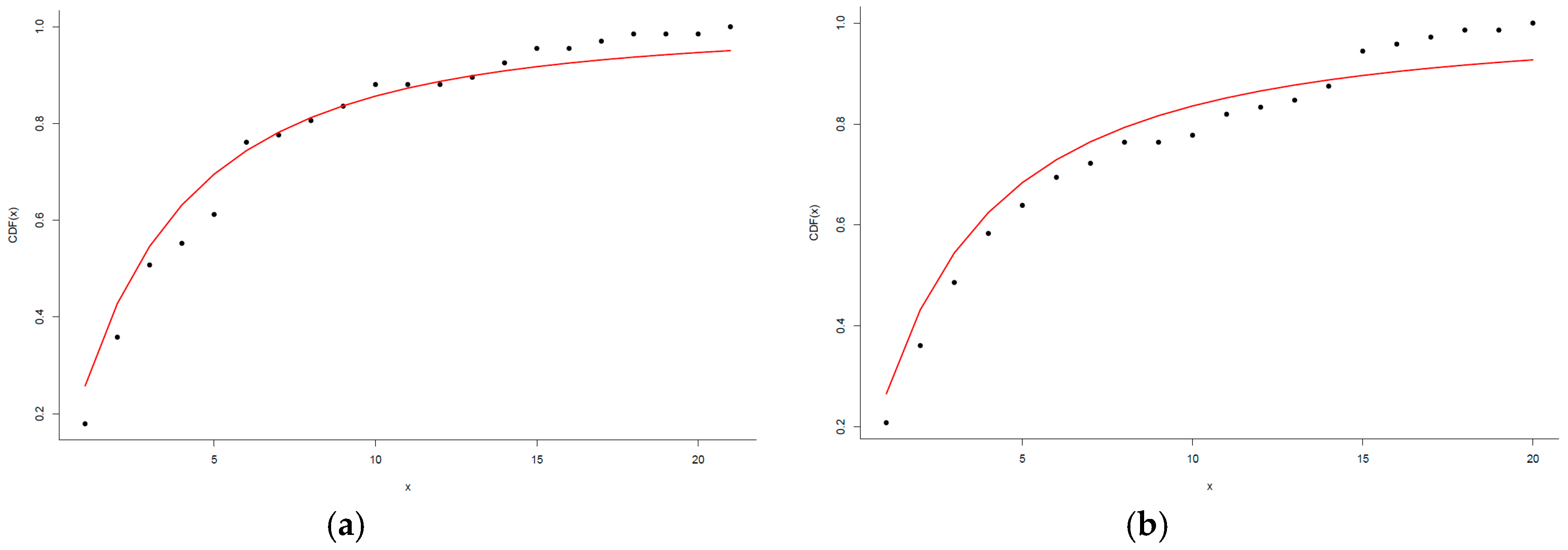
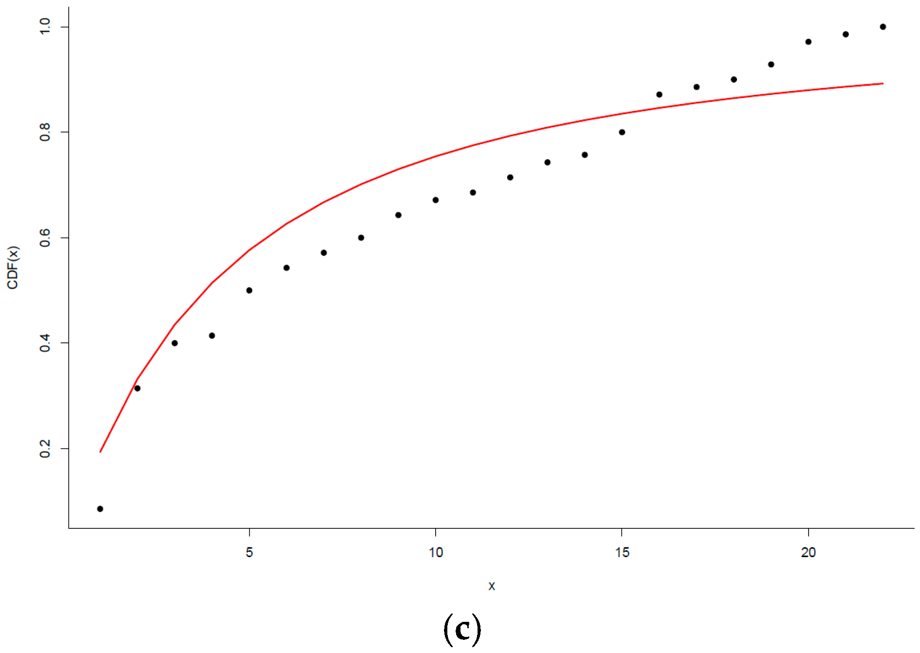
Power-law fit of the degree distribution of the NVGs associated with participants 39, 77, and 103 (points represent the cumulative degree distribution function of the NVG and the red line represents the power-law that best fits the data). (a) NVG degree distribution and power-law fit of participant 39; (b) NVG degree distribution and power-law fit of participant 77; (c) NVG degree distribution and power-law fit of participant 103.
Figure 5.
Power-law fit of the degree distribution of the NVGs associated with participants 39, 77, and 103 (points represent the cumulative degree distribution function of the NVG and the red line represents the power-law that best fits the data). (a) NVG degree distribution and power-law fit of participant 39; (b) NVG degree distribution and power-law fit of participant 77; (c) NVG degree distribution and power-law fit of participant 103.


Figure 6.
Distribution of NVG mean degree by sex.

Figure 7.
Distribution of NVG mean degree by age.

Figure 8.
Ex-Gaussian fit of the RTs of participants 39, 77, and 103 (continuous line represents observed data, dashed line represents fitted data). (a) Ex-Gaussian fit of the RTs of participant 39; (b) Ex-Gaussian fit of the RTs of participant 77; (c) Ex-Gaussian fit of the RTs of participant 103.
Figure 8.
Ex-Gaussian fit of the RTs of participants 39, 77, and 103 (continuous line represents observed data, dashed line represents fitted data). (a) Ex-Gaussian fit of the RTs of participant 39; (b) Ex-Gaussian fit of the RTs of participant 77; (c) Ex-Gaussian fit of the RTs of participant 103.

Figure 9.
The respective NVGs of participants 89, 120, and 84. (a) Natural visibility graph of participant 89; (b) Natural visibility graph of participant 120; (c) Natural visibility graph of participant 84.
Figure 9.
The respective NVGs of participants 89, 120, and 84. (a) Natural visibility graph of participant 89; (b) Natural visibility graph of participant 120; (c) Natural visibility graph of participant 84.

Figure 10.
The respective NVGs of participants 89, 120, and 84 where black nodes represent hits or commission errors and red nodes represent omission errors. (a) Natural visibility graph of participant 89; (b) Natural visibility graph of participant 120; (c) Natural visibility graph of participant 84.


Figure 11.
Power-law fit of the degree distribution of the NVGs associated with participants 89, 120, and 84 (points represent the cumulative degree distribution function of the NVG and the red line represents the power-law that best fits the data). (a) NVG degree distribution and power-law fit of participant 89; (b) NVG degree distribution and power-law fit of participant 120; (c) NVG degree distribution and power-law fit of participant 84.

Figure 12.
Ex-Gaussian fit of RTs of participants 89, 120, and 84 (continuous line represents observed data, dashed line represents fitted data). (a) Ex-Gaussian fit of RTs of participant 89; (b) Ex-Gaussian fit of RTs of participant 120; (c) Ex-Gaussian fit of RTs of participant 84.
Figure 12.
Ex-Gaussian fit of RTs of participants 89, 120, and 84 (continuous line represents observed data, dashed line represents fitted data). (a) Ex-Gaussian fit of RTs of participant 89; (b) Ex-Gaussian fit of RTs of participant 120; (c) Ex-Gaussian fit of RTs of participant 84.


Table 1.
Student distribution by age and sex.
| Age | Females | Males | Total |
|---|---|---|---|
| 8 | 23 (63.9%) | 13 (36.1%) | 36 |
| 9 | 15 (48.4%) | 16 (51.6%) | 31 |
| 10 | 13 (41.9%) | 18 (58.1%) | 31 |
| 11 | 8 (42.1%) | 11 (57.9%) | 19 |
| 12 | 7 (53.8%) | 6 (46.2%) | 13 |
| Overall | 66 (50.8%) | 64 (49.2%) | 130 |
Table 2.
Results of the task by age and sex.
| Age | Sex | Mean No. of Hits | Mean No. of Commission Errors | Mean No. of Omission Errors |
|---|---|---|---|---|
| 8 | Females | 116.1 | 11.6 | 2.1 |
| 8 | Males | 112.6 | 15.3 | 1.8 |
| 9 | Females | 121.5 | 6.8 | 1.5 |
| 9 | Males | 120.5 | 8.4 | 0.8 |
| 10 | Females | 122.0 | 7.1 | 0.6 |
| 10 | Males | 115.4 | 12.8 | 1.3 |
| 11 | Females | 126.1 | 3.7 | 0.1 |
| 11 | Males | 121.5 | 7.9 | 0.4 |
| 12 | Females | 124.9 | 4.8 | 0.3 |
| 12 | Males | 118.2 | 7.3 | 4.5 |
| Overall | Females | 120.6 | 7.9 | 1.2 |
| Overall | Males | 117.4 | 10.9 | 1.4 |
Table 3.
Description of the power-law parameters by age and sex.
| Age | Sex | ||
|---|---|---|---|
| 8 | Females | 4.24 | 2.06 |
| 8 | Males | 4.03 | 1.27 |
| 9 | Females | 4.55 | 2.09 |
| 9 | Males | 4.17 | 1.01 |
| 10 | Females | 4.66 | 2.26 |
| 10 | Males | 4.54 | 2.12 |
| 11 | Females | 3.61 | 0.74 |
| 11 | Males | 5.54 | 1.83 |
| 12 | Females | 5.14 | 2.56 |
| 12 | Males | 4.09 | 1.22 |
| Overall | Females | 4.41 | 2.04 |
| Overall | Males | 4.47 | 1.64 |
Table 4.
Description of the Shannon entropy by age and sex.
| Age | Sex | Mean (h) | SD (h) |
|---|---|---|---|
| 8 | Females | 3.65 | 0.39 |
| 8 | Males | 3.50 | 0.31 |
| 9 | Females | 3.49 | 0.29 |
| 9 | Males | 3.47 | 0.41 |
| 10 | Females | 3.44 | 0.40 |
| 10 | Males | 3.62 | 0.41 |
| 11 | Females | 3.64 | 0.38 |
| 11 | Males | 3.54 | 0.62 |
| 12 | Females | 3.51 | 0.34 |
| 12 | Males | 3.39 | 0.23 |
| Overall | Females | 3.56 | 0.36 |
| Overall | Males | 3.53 | 0.42 |
Table 5.
Description of the ex-Gaussian parameters by age and sex.
| Age | Sex | ||||||
|---|---|---|---|---|---|---|---|
| 8 | Females | 643.4 | 60.55 | 105.34 | 22.88 | 304.10 | 79.17 |
| 8 | Males | 650.7 | 93.61 | 133.18 | 32.14 | 316.00 | 124.5 |
| 9 | Females | 587.5 | 60.97 | 98.62 | 33.99 | 279.89 | 125.6 |
| 9 | Males | 614.9 | 95.29 | 122.33 | 41.63 | 248.00 | 103.0 |
| 10 | Females | 554.3 | 64.48 | 103.58 | 28.96 | 221.67 | 79.67 |
| 10 | Males | 552.6 | 73.77 | 122.91 | 65.99 | 255.10 | 125.9 |
| 11 | Females | 524.9 | 68.43 | 81.06 | 24.12 | 131.90 | 43.79 |
| 11 | Males | 507.4 | 42.39 | 82.43 | 31.46 | 185.54 | 95.39 |
| 12 | Females | 512.9 | 67.19 | 81.15 | 21.24 | 238.20 | 80.92 |
| 12 | Males | 471.3 | 54.36 | 75.83 | 25.72 | 238.04 | 306.2 |
| Overall | Females | 629.5 | 78.30 | 111.50 | 27.86 | 322.87 | 102.6 |
| Overall | Males | 572.7 | 96.78 | 113.48 | 49.22 | 252.15 | 142.1 |
Table 6.
Description of the most extreme cases.
| Participant | Age | Sex | Mean Reaction Time | # Hits | # Omission Errors | # Commission Errors | Shannon Entropy |
|---|---|---|---|---|---|---|---|
| 89 | 12 | M | 1338.7* | 91 | 27 | 12 | 3.44 |
| 120 | 8 | F | 974.5 | 14 | 7 | 109* | 3.92 |
| 84 | 12 | M | 492.7* | 124 | 0 | 6 | 3.12 |
Table 7.
Power-law and ex-Gaussian parameters of the most extreme cases.
| Participant | ||||
|---|---|---|---|---|
| 89 | 5.8 | 481.9 | 46.9 | 856.9 |
| 120 | 2.2 | 580.5 | 136.8 | 394.0 |
| 84 | 3.2 | 437.8 | 54.1 | 54.85 |
© 2019 by the authors. Licensee MDPI, Basel, Switzerland. This article is an open access article distributed under the terms and conditions of the Creative Commons Attribution (CC BY) license (http://creativecommons.org/licenses/by/4.0/).
Share and Cite
MDPI and ACS Style
Mira-Iglesias, A.; Navarro-Pardo, E.; Conejero, J.A. Power-Law Distribution of Natural Visibility Graphs from Reaction Times Series. Symmetry 2019, 11, 563. https://doi.org/10.3390/sym11040563
AMA Style
Mira-Iglesias A, Navarro-Pardo E, Conejero JA. Power-Law Distribution of Natural Visibility Graphs from Reaction Times Series. Symmetry. 2019; 11(4):563. https://doi.org/10.3390/sym11040563
Chicago/Turabian StyleMira-Iglesias, Ainara, Esperanza Navarro-Pardo, and J. Alberto Conejero. 2019. "Power-Law Distribution of Natural Visibility Graphs from Reaction Times Series" Symmetry 11, no. 4: 563. https://doi.org/10.3390/sym11040563
Note that from the first issue of 2016, this journal uses article numbers instead of page numbers. See further details here.