Null Electromagnetic Fields from Dilatation and Rotation Transformations of the Hopfion


1
Área de Electromagnetismo, Universidad Rey Juan Carlos, Calle Tulipán s/n, 28933 Móstoles (Madrid), Spain
2
Departamento de Física Aplicada III, Universidad Complutense, Plaza de las Ciencias s/n, 28040 Madrid, Spain
3
Instituto de Física Fundamental, Consejo Superior de Investigaciones Científicas, Calle Serrano 113, 28006 Madrid, Spain
*
Author to whom correspondence should be addressed.
†
These authors contributed equally to this work.
Symmetry 2019, 11(9), 1105; https://doi.org/10.3390/sym11091105
Submission received: 22 July 2019
/
Revised: 19 August 2019
/
Accepted: 28 August 2019
/
Published: 2 September 2019
(This article belongs to the Special Issue Symmetry in Electromagnetism)
Abstract
:The application of topology concepts to Maxwell equations has led to the developing of the whole area of electromagnetic knots. In this paper, we apply some symmetry transformations to a particular electromagnetic knot, the hopfion field, to get a new set of knotted solutions with the properties of being null. The new fields are obtained by a homothetic transformation (dilatation) and a rotation of the hopfion, and we study the constraints that the transformations must fulfill in order to generate valid electromagnetic fields propagating in a vacuum. We make use of the Bateman construction and calculate the four-potentials and the electromagnetic helicities. It is observed that the topology of the field lines does not seem to be conserved as it is for the hopfion.
1. Introduction
In recent years, topology ideas applied to physics have provided useful insights into many different phenomena, ranging from phase transitions to solid state physics, superfluids, and magnetism. The topology applied to electromagnetism has opened the field of electromagnetic knots [1], where light gets nontrivial properties. One example of a electromagnetic knot is the hopfion.
The hopfion is an exact null solution of the Maxwell equations in a vacuum [1,2,3,4]. The null property means that the Lorentz invariants of the field are zero, i.e., and [5]. The hopfion is characterized by further special properties such as the field lines being closed and linked for any instant of time. The topology of the field lines is described for any time in terms of two complex scalar fields and . The solution of and , with complex constants, gives all the magnetic and electric lines (by changing the value of the constant at the right-hand side), which are linked closed lines topologically equivalent to circles. In particular, for the hopfion, those complex fields can be written in terms of four real scalar fields , as:
The ’s satisfy the conditions and , so they can be considered as time-dependent coordinates on the sphere . In this case, the and are then applications from , and the linking properties of the field lines follow from this fact [1].
In this paper, we apply some symmetry transformations to the hopfion. In particular, we make a homothetic transformation (dilatation) and a rotation of the hopfion at a particular time. We find that those transformations cannot be arbitrary in order for the transformed fields to be still electromagnetic solutions. We provide the conditions required for the transformations. We give explicit expressions for the new null fields for any time using the Bateman construction. Furthermore, the four-potentials of the new fields and the electromagnetic helicities are calculated. The non-null helicities point to the fact that the topology of the field lines is not trivial. However, the new solutions do not seem to preserve the closedness property of the hopfion field lines. This fact deserves future investigations.
2. Topological Construction of Vacuum Solutions and the Hopfion Field
In this section, we will briefly revise a topological formulation of electromagnetism in a vacuum built in [3,6,7,8] and give the explicit expression for the hopfion field. We will make use of certain properties of this construction in the next section when we apply the transformations to the hopfion.
Solutions of Maxwell equations in a vacuum (we will use MKSunits),
can be found from a pair of complex scalar fields and , so the magnetic end electric fields are given by:
As usual, c denotes the speed of light, and a is a constant so that the magnetic and electric fields have correct dimensions in MKS units since and are dimensionless ( is the complex conjugate of ). Equation (3) follows from the first equality of Equation (7). Equation (4) is found using the first equality of Equation (7) and the second equality of Equation (8). Equation (5) comes from the first equality of Equation (8). Equation (6) is fulfilled considering the second equality of Equation (7) and the first equality of Equation (8).
To get a solution of Maxwell equations in a vacuum, the complex scalar fields and have to be found to satisfy Equations (7) and (8), so:
These equations are a bit cumbersome, although some solutions have been found in the literature [2,3,9]. On the other side, the advantage of this formulation is that the magnetic and the electric lines are very easily obtained. The field lines at a given time t correspond to the level curves of the scalar field and . This observation can be particularly useful to find solutions of Maxwell equations in a vacuum in which the magnetic and electric lines form knotted curves [1,3]. In this case, the degree of knottedness has interesting physical consequences [4,10,11,12,13,14,15,16].
All the solutions of Maxwell equations in this particular formulation satisfy the Lorentz-invariant equation . This can be immediately seen by using the first equality of Equation (7) and the second equality of Equation (8) or, correspondingly, the second equality of Equation (7) and the first equality of Equation (8). However, it is not true that all the solutions in this formulation satisfy the other null condition, .
The hopfion was found choosing the particular form Equation (1) for and Equation (2) for . In terms of the four real scalar fields , , , , using Equations (7) and (8) turns out to be:
The explicit expressions for the ’s are:
where:
and are dimensionless coordinates. Spacetime coordinates are related to them as:
being a constant with length dimensions, which characterizes the mean quadratic radius of the electromagnetic energy distribution [17].
It is easy to see, given Expressions (13)–(16), that the ’s satisfy the conditions and for any time. For the hopfion, both null conditions and are satisfied.
3. Dilatation and Rotation of the Hopfion
In this section, we explore the possibility of obtaining new solutions by symmetry transformations. We will apply a family of transformations to the hopfion: a dilatation and a rotation at a particular time. We then check the conditions imposed by the initial conditions of Maxwell solutions to find that the transformations must fulfill some constraints expressed as differential equations. The equations are then solved in order to determine a particular set of allowed transformations. In the next section, we will extend the results to every time and generate a more general transformation of the hopfion field that satisfies Maxwell equations in a vacuum.
A warning: along this section, the notation is simplified by taking , , , and we will write coordinates as , respectively, in all the computations. However, the final results will be written back with all the constants, so that they can be used in different contexts.
The particular time is chosen to apply the transformations as the expressions are simpler. The hopfion at this particular time can be written using the new notation as:
and the Poynting vector reads:
where the vector fields:
have been defined. They constitute a basis in the three-dimensional Euclidean space, satisfying:
We will make, as stated above, a dilatation and rotation of the fields and write the transformed fields as:
where f is a function of and is a function of .
In order for the new fields to be a solution of Maxwell equations in a vacuum (see the previous section), it is necessary for Equation (23) to satisfy the equations:
from which, given that and , we get:
Let us define . Since ,
where we use the notation:
Since , , form one basis of three-dimensional vectors Equation (22), we can write, using Equation (29),
where we have defined . Using Equation (21),
so that:
where:
We apply now the curl and project to the direction, i.e, we apply the operator to Expression Equation (32). With the help of Equations (21) and (22), we obtain after some manipulations:
where . This shows that depends only on and , so that:
Expressions Equations (36) and (37) can be simplified, and using Equation (34) to compute , the previous system can be written as:
The solution of this system of equations is:
which, after integration, gives:
where m is an integration constant that can be any real number. Inserting these solutions into Equation (32), after integration, is found to be:
and using Equations (44) and (27) to solve for f gives:
where we have chosen the constants of integration so that this particular value is obtained.
4. Bateman Formulation
After finding the fields at a particular time, we need to extend them to any time. To get the time-dependent expressions of the transformed fields Equation (48), we will make use of the Bateman formulation of null electromagnetic fields in a vacuum. In this section, we review very briefly Bateman’s method.
In the case of Maxwell equations in a vacuum, it is useful to consider, instead of the magnetic and the electric fields separately, a complex combination of them called the Riemann–Silberstein vector [18], which can be written as:
where c appears due to the different units of the magnetic and the electric fields. In terms of , Maxwell equations in a vacuum Equations (3)–(6) read:
The following expressions hold for the Riemann–Silberstein vector using Equations (7) and (8),
The formulation of electromagnetic fields constructed by Bateman in 1915 [19] can be used to study all null solutions of Maxwell equations in a vacuum [20]. The basic fields in this formulation are two complex functions and so that the Riemann–Silberstein vector of the electromagnetic field is written as:
where the factor is chosen so that the comparison with the same vector Equation (52) is more direct. As a consequence, and are dimensionless functions of space and time.
Maxwell equations in a vacuum Equations (50) and (51) are satisfied by the electromagnetic field Equation (53) provided can be also written as:
Equation is satisfied by using Equation (53). To get the Maxwell equation , one can use Equation (54) in the left-hand side and Equation (53) in the right-hand side. The problem of finding solutions of Maxwell equations in a vacuum in the Bateman formulation is then reduced to solving the complex equation:
for the complex fields and . A property of the electromagnetic fields in a vacuum constructed using the Bateman formulation is that they are null. Multiplying Equations (53) and (54), it is easily seen that , so defines a null electromagnetic field in a vacuum ( and ).
We now obtain the hopfion in the Bateman formulation Equations (53) and (54). This was first obtained by Besieris and Shaarawi [21] and later by Kedia et al. [22] and Hoyos et al. [23], among others. Our results will be completely equivalent to the ones obtained in those references, although slightly different, since we are going to use Equations (11) and (12). We begin by writing the Riemann–Silberstein vector of the hopfion, using Equations (11) and (12), as:
Making use of the values of the real scalar fields Equations (13) and (16), we get:
Note that the results Equation (57) coincide with the ones found in [22] with changes and , due to a different labeling of the axes.
An interesting observation about the Bateman formulation that we will use in this work is the following: every electromagnetic field constructed from a solution of Maxwell’s equations in a vacuum Equations (50) and (51) as:
where is an arbitrary function of the complex fields and is also a solution [19].
This property was exploited by Kedia et al. in [22] to find a set of null solutions of the Maxwell equations in a vacuum that generalize the Hopfion and give field lines that are linked torus knots at . The solutions they found can be written in the Bateman formulation Equations (53) and (54) using two positive integer numbers m and n as:
Further generalizations for generating other fields can be found in [23].
5. A New Set of Null Electromagnetic Fields
In this section, we extend the transformations for the fields given by Equation (48) at a particular time to any time exploiting the properties of the Bateman formulation we have just reviewed in the previous section. Thus, we will get the new set of null electromagnetic fields.
As pointed out earlier, the Riemann–Silberstein vector allows writing the transformed fields at a particular time in a very compact form, which sheds some light on the transform valid for any time. For the transformed fields at Equation (48), we get:
being the Riemann–Silberstein vector of the hopfion at , i.e.,:
The key point is to observe that we can write Equation (63) as:
where, according to Equations (14) and (16), and are, respectively, the values of and at .
Invoking the property Equation (58), we can extend the transformed fields for all time:
where and are given by Equations (14) and (16) and is the Riemann–Silberstein vector of the Hopfion Equation (56). This means that we can express as:
Moreover, we can generalize this solution by playing the same game with the complex field . We arrive then at our final expression for a new set of electromagnetic fields constructed from the hopfion by dilation and rotation. These fields are given by the Riemann–Silberstein vector defined as:
that, by construction, are null electromagnetic fields and satisfy Maxwell equations in a vacuum when , , , are the ones defined in Expressions (13)–(16). In a more compact notation,
This expression shows what kind of new solutions have been found. They correspond to a dilation of the magnetic and electric fields of the Hopfion plus a rotation in the plane . Both the dilation and the rotation parameters depend on the ’s variables and on the two constants m and n, which can be seen by writing the new solutions as:
6. Four-Potentials and Helicities
The Bateman formalism is also to find the electromagnetic four-potentials for the solutions that can be written as in Equations (53) and (54). In this section, we will give the recipe and calculate them for the new solutions obtained in the previous section.
It is standard to define the electromagnetic four-potential in Minkowski spacetime, with and a metric given by diagonal elements , so that , . It is possible only in a vacuum to define (see [1] for example) a second electromagnetic potential that satisfies , . Let us consider the complex combination:
Then, the Riemann–Silberstein vector satisfies:
Now, consider the situation in which the electromagnetic field can be written in the Bateman formalism as:
We have also a gauge degree of freedom to choose any other electromagnetic potential from Equation (75) as:
The magnetic and electric helicities [24] of an electromagnetic field in a vacuum can be defined, in angular momentum units, as:
where is the electric permittivity of a vacuum. The magnetic helicity measures the mean value of the Gauss linking number of the magnetic field lines [25], and the electric helicity plays the same role for the electric field. For null electromagnetic fields in a vacuum, , and moreover, both helicities remain independent of time [2]. For an electromagnetic field expressed in the Bateman formalism as Equation (74) with the electromagnetic potential given by Equation (75), it is trivial to check that:
showing that we are in the case of null fields.
The sum of both helicities is the electromagnetic helicity [26],
and it can be written in the Bateman formalism using again Equations (74) and (75) as:
with a bar over a letter meaning complex conjugation.
In particular, for the hopfion Equation (56), we have, due to Equation (57), for the potential Equation (75),
results that are, except a gauge transformation, similar to the ones found in [27]. The electromagnetic helicity of the hopfion, according to Equation (80), results in:
which can be taken as the unit of electromagnetic helicity for the hopfion and related electromagnetic fields in a vacuum [24].
Let us consider now the electromagnetic potential of the solutions Equation (71) found in the previous section. For them,
and from Equation (75), the potentials read:
where the ’s are given in Equations (13)–(16). The magnetic and electric helicities of these solutions have the same value, since the field is null. The electromagnetic helicity is, according to Equations (80) and (82):
7. Conclusions
In this work, we studied symmetry transformations at a particular time for generating new solutions of Maxwell equations in a vacuum. The transformations need to satisfy some constraints. We then made use of the Bateman formulation to get new null electromagnetic fields at any time.
Another important result presented was the method of using the Bateman formulation to find the electromagnetic potentials for null solutions of Maxwell equations in a vacuum. This method allowed us to compute their magnetic and electric helicities.
We found numerically that the topology seemed to not be conserved, and the closedness of the electric and magnetic field lines was broken for the new fields. This is a fact that has been observed in other solutions that used the hopfion and the Bateman construction for generating other fields [22]. However, we cannot exclude that it was due to numerical accuracy. This point together with the linking of the field lines deserves future investigation, and it might shed some light on the complex dynamics of these knotted fields and how to generate them in the laboratory.
The research on electromagnetic knots belongs to the research of the classical theory of particles and fields, but the techniques and concepts involved might be extended to other areas, such as dynamical systems, liquid crystals, stellar plasma configurations, topological insulators, etc. Many of the consequences remain to be explored.
Author Contributions
All the authors contributed equally to all the parts of this work.
Funding
This research was funded by the Spanish Ministry of Economy and Competitiveness grant number ESP2017-86263-C4-3-R.
Conflicts of Interest
The authors declare no conflict of interest.
References
- Arrayás, M.; Bouwmeester, D.; Trueba, J.L. Knots in electromagnetism. Phys. Rep. 2017, 667, 1–61. [Google Scholar] [CrossRef] [Green Version]
- Rañada, A.F.; Trueba, J.L. Two properties of electromagnetic knots. Phys. Lett. A 1997, 232, 25–33. [Google Scholar] [CrossRef]
- Rañada, A.F.; Trueba, J.L. Topological Electromagnetism with Hidden Nonlinearity. In Modern Nonlinear Optics, 3rd ed.; Evans, M.W., Ed.; John Wiley & Sons: New York, NY, USA, 2001; pp. 197–253. [Google Scholar]
- Irvine, W.T.; Bouwmeester, D. Linked and knotted beams of light. Nat. Phys. 2008, 4, 716–720. [Google Scholar] [CrossRef] [Green Version]
- Robinson, I. Null electromagnetic fields. J. Math. Phys. 1961, 2, 290. [Google Scholar] [CrossRef]
- Rañada, A.F. A topological theory of the electromagnetic field. Lett. Math. Phys. 1989, 18, 97–106. [Google Scholar] [CrossRef]
- Rañada, A.F. Knotted solutions of the Maxwell equations in vacuum. J. Phys. A Math. Gen. 1990, 23, L815. [Google Scholar] [CrossRef]
- Rañada, A.F. Topological electromagnetism. J. Phys. A Math. Gen. 1992, 25, 1621. [Google Scholar] [CrossRef]
- Rañada, A.F.; Trueba, J.L. Electromagnetic knots. Phys. Lett. A 1995, 202, 337–342. [Google Scholar] [CrossRef]
- Irvine, W.T.M. Linked and knotted beams of light, conservation of helicity and the flow of null electromagnetic fields. J. Phys. A Math. Theor. 2010, 43, 385203. [Google Scholar] [CrossRef]
- Dalhuisen, J.W.; Bouwmeester, D. Twistors and electromagnetic knots. J. Phys. A Math. Theor. 2012, 45, 135201. [Google Scholar] [CrossRef]
- Arrayás, M.; Trueba, J.L. Exchange of helicity in a knotted electromagnetic field. Ann. Phys. 2012, 524, 71–75. [Google Scholar] [CrossRef]
- Enk, S.J. Covariant description of electric and magnetic field lines of null fields: Application to Hopf-Rañada solutions. J. Phys. A Math. Theor. 2013, 46, 175204. [Google Scholar] [CrossRef]
- Arrayás, M.; Trueba, J.L. A class of non-null toroidal electromagnetic fields and its relation to the model of electromagnetic knots. J. Phys. A Math. Theor. 2015, 48, 025203. [Google Scholar] [CrossRef]
- Arrayás, M.; Trueba, J.L. Collision of two hopfions. J. Phys. A Math. Theor. 2017, 50, 085203. [Google Scholar] [CrossRef] [Green Version]
- Arrayás, M.; Trueba, J.L. On the fibration defined by the field lines of a knotted class of electromagnetic fields at a particular time. Symmetry 2017, 9, 218. [Google Scholar] [CrossRef]
- Arrayás, M.; Trueba, J.L. Motion of charged particles in a knotted electromagnetic field. J. Phys. A 2010, 43, 235401. [Google Scholar] [CrossRef]
- Bialynicki-Birula, I.; Bialynicka-Birula, Z. The role of the Riemann-Silberstein vector in Classical and Quantum Theories of Electromagnetism. J. Phys. A Math. Theor. 2013, 46, 053001. [Google Scholar] [CrossRef]
- Bateman, H. The Mathematical Analysis of Electrical and Optical Wave-Motion; Dover: New York, NY, USA, 1915. [Google Scholar]
- Hogan, P. Bateman electromagnetic waves. Proc. R. Soc. A 1984, 396, 199. [Google Scholar] [CrossRef]
- Besieris, I.M.; Shaarawi, A. Hopf-Rañada linked and knotted light beam solution viewed as a null field. Opt. Lett. 2009, 34, 3887–3889. [Google Scholar] [CrossRef]
- Kedia, H.; Bialinicki-Birula, I.; Peralta-Salas, D.; Irvine, W.T.M. Tying knots in beams of light. Phys. Rev. Lett. 2013, 111, 150404. [Google Scholar] [CrossRef]
- Hoyos, C.; Sircar, N.; Sonnenschein, J. New knotted solutions of Maxwell’s equations. J. Phys. A 2015, 48, 255204. [Google Scholar] [CrossRef]
- Arrayás, M.; Trueba, J.L. Spin-Orbital momentum decomposition and helicity exchange in a set of non-null knotted electromagnetic fields. Symmetry 2018, 10, 88. [Google Scholar] [CrossRef]
- Moffatt, H.K.; Ricca, R.L. Helicity and the Calugareanu Invariant. Proc. R. Soc. Lond. A 1992, 439, 411–429. [Google Scholar] [CrossRef]
- Trueba, J.L.; Rañada, A.F. The electromagnetic helicity. Eur. J. Phys. 1996, 17, 141. [Google Scholar] [CrossRef]
- Rañada, A.F.; Tiemblo, A.; Trueba, J.L. Time evolving potentials for electromagnetic knots. Int. J. Geom. Methods Mod. Phys. 2017, 14, 1750073. [Google Scholar] [CrossRef] [Green Version]
Figure 1.
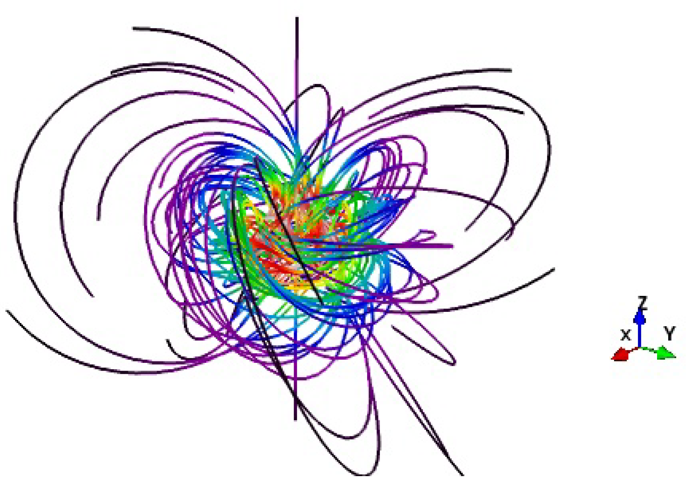
In the first figure (top), we represent some magnetic field lines for the initial value (t = 0) of the hopfion field, which corresponds to a value m = 0 in Equation (48). All the magnetic lines drawn are closed and linked to each other, which is the defining property of this field. In the second figure (middle), we plot some magnetic field lines for the transformed field with m = 1 in Equation (48), and in the third figure (bottom), some magnetic field lines for the transformed field with m = 2 in Equation (48) are drawn. The magnetic lines for the cases m = 1 and m = 2 seem to be unclosed in the numerics that give the lines plotted in the second and third figures.
Figure 1.
In the first figure (top), we represent some magnetic field lines for the initial value (t = 0) of the hopfion field, which corresponds to a value m = 0 in Equation (48). All the magnetic lines drawn are closed and linked to each other, which is the defining property of this field. In the second figure (middle), we plot some magnetic field lines for the transformed field with m = 1 in Equation (48), and in the third figure (bottom), some magnetic field lines for the transformed field with m = 2 in Equation (48) are drawn. The magnetic lines for the cases m = 1 and m = 2 seem to be unclosed in the numerics that give the lines plotted in the second and third figures.


Figure 2.
Same as Figure 1, but considering electric field lines. In the first figure (top), we represent electric field lines for the initial value (t = 0) of the hopfion field, all of which are closed and linked to each other. In the second figure (middle), we plot electric field lines for the transformed field with m = 1 in Equation (48), and in the third figure (bottom), we plot some electric field lines for the transformed field with m = 2 in Equation (48). The electric lines for the cases m = 1 and m = 2 seem to be unclosed in the numerics.


Figure 3.
In this figure, we represent some magnetic field lines for the initial value () of the magnetic field given in Equation (71) with values and . As in the cases shown in the second and third plots of Figure , these magnetic lines seem to be unclosed in the numerics.
Figure 3.
In this figure, we represent some magnetic field lines for the initial value () of the magnetic field given in Equation (71) with values and . As in the cases shown in the second and third plots of Figure , these magnetic lines seem to be unclosed in the numerics.

Figure 4.
Same as Figure 3, but considering electric field lines. We plot some electric field lines for the initial value () of the electric field given in Equation (71) with values and . As in the cases shown in the second and third plots of Figure 2, these electric lines seem to be unclosed in the numerics.

© 2019 by the authors. Licensee MDPI, Basel, Switzerland. This article is an open access article distributed under the terms and conditions of the Creative Commons Attribution (CC BY) license (http://creativecommons.org/licenses/by/4.0/).
Share and Cite
MDPI and ACS Style
Arrayás, M.; Rañada, A.F.; Tiemblo, A.; Trueba, J.L. Null Electromagnetic Fields from Dilatation and Rotation Transformations of the Hopfion. Symmetry 2019, 11, 1105. https://doi.org/10.3390/sym11091105
AMA Style
Arrayás M, Rañada AF, Tiemblo A, Trueba JL. Null Electromagnetic Fields from Dilatation and Rotation Transformations of the Hopfion. Symmetry. 2019; 11(9):1105. https://doi.org/10.3390/sym11091105
Chicago/Turabian StyleArrayás, Manuel, Antonio F. Rañada, Alfredo Tiemblo, and José L. Trueba. 2019. "Null Electromagnetic Fields from Dilatation and Rotation Transformations of the Hopfion" Symmetry 11, no. 9: 1105. https://doi.org/10.3390/sym11091105
Note that from the first issue of 2016, this journal uses article numbers instead of page numbers. See further details here.