Relativistic Gravitation Based on Symmetry

Abstract

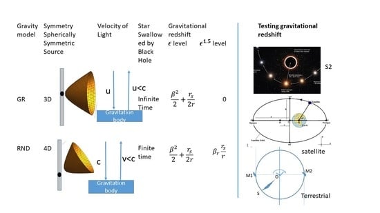
We present a Relativistic Newtonian Dynamics ($RND$) for motion of objects in a gravitational field generated by a moving source. As in General Relativity ($GR$), we assume that objects move by a geodesic with respect to some metric, which is defined by the field. This metric is defined on flat lab spacetime and is derived using only symmetry, the fact that the field propagates with the speed of light, and the Newtonian limit. For a field of a single source, the influenced direction of the field at spacetime point x is defined as the direction from x to the to the position of the source at the retarded time. The metric depends only on this direction and the strength of the field at x. We show that for a static source, the $RND$ metric is of the same form as the Whitehead metric, and the Schwarzschild metric in Eddington–Finkelstein coordinates. Motion predicted under this model passes all classical tests of $GR$. Moreover, in this model, the total time for a round trip of light is as predicted by $GR$, but velocities of light and object and time dilation differ from the $GR$ predictions. For example, light rays propagating toward the massive object do not slow down. The new time dilation prediction could be observed by measuring the relativistic redshift for stars near a black hole and for sungrazing comets. Terrestrial experiments to test speed of light predictions and the relativistic redshift are proposed. The $RND$ model is similar to Whitehead’s gravitation model for a static field, but its proposed extension to the non-static case is different. This extension uses a complex four-potential description of fields propagating with the speed of light.

1. Introduction

Einstein’s General Relativity ($GR$) has succeeded in explaining non-classical behavior in astrophysics. $GR$ successfully implements Riemann’s idea “force equals geometry” to gravitation. In $GR$, the gravitational force curves spacetime. The curving of spacetime is expressed by a metric [1,2,3]. By the Equivalence Principle, this metric is the same for all objects. It is assumed the motion of any object, massive or massless, is by a geodesic with respect to this metric. Einstein’s field equations, which is a set of nonlinear partial differential equations, are used to define the metric from the sources of the field.

In 1922, A. N. Whitehead published [4] a relativistic theory of gravity, much simpler than $GR$ and containing no arbitrary parameters. This theory is set in Minkowski spacetime, and it is assumed that the motion of any object is by a geodesic with respect to a metric defined on this spacetime. The metric describes the gravitational field, and, assuming that the field propagates with the speed of light, it is defined by the position of the sources at the retarded time. Whitehead proposed a metric for a static, spherically symmetric gravitation field, which we call the Whitehead metric. This metric differs from the corresponding $GR$ metric—the Schwarzschild metric [5]. Whitehead showed that the dynamics based on this metric accurately predicts the anomalous precession of the perihelion of Mercury and the deflection of light.

In 1924, A. S. Eddington [6] showed that in new coordinates on spacetime, now called Eddington- Finkelstein coordinates, the Whitehead metric coincides with the Schwarzschild metric. Finkelstein arrived at these coordinates [7] while showing that the Schwarzschild radius is only a coordinate singularity and not a true physical singularity. A complexification of the Whitehead metric was used by Kerr [8] to obtain an exact solution of Einstein field equations for a rotating, axially-symmetric massive object, see also [9]. In 1952, J. L. Synge [10] presented an explicit form for Whitehead’s metric for a field generated by several sources. From that time until the present, there is a difference of opinion whether Whitehead’s theory of gravitation violates experimental tests, see [11,12,13] and references therein.

In this paper, we present a Relativistic Newtonian Dynamics (RND) for a gravitational field. An earlier version was developed by the author and others [14,15,16,17,18,19,20,21,22,23]. $RND$ is an attempt to realize Riemann’s program for all forces. It is a metric-based Lagrangian theory. This theory is similar to Whitehead’s theory of gravitation for a single static source, but the interpretation and the derivation of the metric is different. In this paper, we lay out the ideas behind $RND$ and apply our model to the motion of an object in a static, spherically symmetric field.

The key point in deriving the metric of such a field is the use the symmetry of the problem resulting because the field propagates with the speed of light. The symmetry defines the form of the metric up to an unknown function, which is determined by the Newtonian limit. The obtained metric is Whitehead’s metric. The trajectories predicted by $RND$ and $GR$ are the same. The $RND$ model passes all solar tests of $GR$. The total round trip time of light for both models is the same. Thus, round-trip experiments cannot distinguish between $RND$ and $GR$.

In contrast to Whitehead’s theory, $RND$ makes predictions different from $GR$ for the relativistic redshift. The $GR$ metric is invariant under time reversal, but the $RND$ metric breaks the time reversal symmetry. The differences in the predicted relativistic redshift could be observed for stars near a black hole. This redshift was recently measured and analyzed for the SO-2 star near the massive black hole at the center of the Milky Way galaxy. The differences in the relativistic redshift could also be observed for sungrazing comets. The velocities of objects in $RND$ differ from those predicted by $GR$. In $RND$, a star can be swallowed by a black hole in finite time, whereas in $GR$, this will take infinite time.

In a strong, static gravitational field, $RND$ predicts a different one-way speed of light from that predicted by $GR$. For instance, the speed of light toward the gravitational source is always c, and is not slowed down, as in $GR$. These predictions have not yet been tested. We propose two experiments: one to test the one-way speed of light and a second to test relativistic redshift predictions.

In Section 9, we reveal the shortcomings of Whitehead’s treatment of a non-static source. We propose how to extend $RND$ to a non-static force field. This extension is based on the pre-potential and four-potential description on a field propagating with the speed of light, see [24].

2. The Ideas behind Relativistic Newtonian Dynamics

To describe dynamics by use of geometry one must consider trajectories in spacetime, not in space. For example, free or constant velocity motion an object is described by a a straight line in spacetime, while knowing that its trajectory is a straight line in space tells nothing about the objects acceleration. We describe the motion of objects with respect to a preferred frame, called the lab frame, as observed by an observer far away from the sources of the field. We will assume that the lab frame is in Minkowski spacetime.

We always have a preferred frame of reference. For example, if we are considering the motion of Mercury, we use a frame with the Sun at the center and measure distances with respect to the background of fixed stars. If we are dealing with motion within a distant galaxy, we observe this motion from a point far away from the field within the galaxy, and we may use the frame represented by the microwave background radiation [25,26].

The development of our dynamics starts with the relativity of spacetime, which mean that spacetime is an object-dependent notion. The objects spacetime is defined by the forces affecting it. For example, an electron and a neutron exist in different worlds in the vicinity of an electric field. The electric field does not exist for the neutron. The way spacetime curves due to an electric potential depends also on intrinsic properties of the object. This was also recognized in [27] in the geometric approach of electrodynamics. For gravity, by the Equivalence Principle, a gravitational field is felt equally by all objects. Therefore, the geometry of the field is object independent.

How does the field affect an object’s motion? The motion of an object is described by its world-line in the lab frame K. If there is no field around, the four-acceleration a observed in K is zero. If there is a field affecting the object’s motion, the field will define the acceleration on the world-line. As the admissible speeds in relativity are limited by the speed of light, in any relativistic dynamics, unlike in Newtonian dynamics, the acceleration must depend also on the four-velocity u of the moving object.

We are aware of two ways in which the four-acceleration a can depend on the four-velocity u. The first one is linear dependence. For example, for an electromagnetic field, the acceleration caused by the Lorentz force is $a=Fu$, where F is an antisymmetric $4\times 4$ tensor. Motion under such dynamics predicts a precession for motion in a central field, but this precession is much smaller that the observed anomalous precession of Mercury’s orbit. Thus, dynamics based on linear dependence on u cannot properly describe the gravitational field. The second type of dependence arises in geodesic motion with respect to some metric. For such motion, the dependence of a on u is quadratic. Such dynamics properly predicts the anomalous precession of Mercury’s orbit. Thus, as in $GR$, we assume that the geometry of spacetime caused by a gravitational field is defined by a metric. As the speed of propagation of the field is finite, this metric at a given time will be defined by the position of the sources of the field in the past.

We maintain that an object moves freely in its spacetime. In other words, the object’s acceleration is zero in a spacetime defined by the force, that is, it moves along a geodesic with respect to the metric defined by the field. This results from the fact that an inanimate object has no internal mechanism to change its velocity. Thus, in its world, its acceleration is zero. Note that $GR$ makes the same claim about an object freely falling in a gravitational field.

We should also emphasize here how our approach differs from $GR$. The first, and primary, difference is perspective. We work in flat spacetime. In $GR$, one works in curved spacetime, on a pseudo-Riemannian manifold. The assumption is that one can, in fact, carry out measurements in curved spacetime. The standard $GR$ definition of the radial coordinate r (see for example [2,28]) is to define it so that a sphere of radius r has surface area $4\pi r^2$. However, how are we to measure surface area in curved spacetime? Our approach, on the other hand, is to measure r in a well-defined inertial frame far removed from the sources. This is what is measured usually.

As a geodesic has minimal length, it is advantageous to use a variational principle: We will derive Euler–Lagrange-type equations and obtain conservation of certain momenta. With these tools, we can compute the metric. Let the line element of the spacetime metric be

$$d{s}^2=g_{\alpha \beta }\left(q\right)d{q}^{\alpha }d{q}^{\beta },$$

(1)

where $q^{\alpha },\alpha =0,1,2,3$ are the coordinates in an inertial lab frame K. Introduce the function L

$$L\left(q,\acute{q}\right)=c\sqrt{g_{\alpha \beta }\left(q\right){\acute{q}}^{\alpha }{\acute{q}}^{\beta }}$$

(2)

with independent variables $q^{\alpha },{\acute{q}}^{\alpha }$:

We describe a trajectory of an object of mass m by $q:\sigma \to x,a\le \sigma \le b,$ with an arbitrary parameter $\sigma$. The length of the trajectory $l\left(q\right)$ is given by

$$l\left(q\right)=c{\int }_a^b\frac{ds}{d\sigma }d\sigma ={\int }_a^{b}L\left(q,\frac{dq}{d\sigma }\right)d\sigma .$$

(3)

The length of a perturbation of the trajectory $r:\sigma \to x,a\le \sigma \le b,r\left(a\right)=r\left(b\right)=0$ is extremal if

$$\frac{d}{dϵ}{l(q+ϵr)|}_{ϵ=0}=0.$$

(4)

As the object moves along a geodesic, the length of the trajectory $q\left(\sigma \right)$ is extremal. By a standard argument, using integration by parts, it follows that $q\left(\sigma \right)$ satisfies the Euler–Lagrange equations

$$\frac{\partial L}{\partial q^{\mu }}-\frac{d}{d\sigma }\frac{\partial L}{\partial {\acute{q}}^{\mu }}=0,$$

(5)

where L is defined by (2) and $\acute{q}=\frac{dq}{d\sigma }$. In this case, the conjugate momentum $u_{\mu }$ per unit mass is

$$u_{\mu }=\frac{\partial L}{\partial {\acute{q}}^{\mu }}{|}_{\acute{q}=\frac{dq}{d\sigma }}=\frac{c{g}_{\mu \beta }\frac{d{q}^{\beta }}{d\sigma }}{ds/d\sigma }=c{g}_{\mu \beta }\frac{d{q}^{\beta }}{ds}.$$

(6)

The second term in Equation (5) contains differentiation is by s, as seen in Equation (6) first and then differentiation is by $\sigma$. To obtain a differential equation with a single parameter, we choose $\sigma$ to be proportional to s. More precisely, we choose $\sigma$ to be the “proper time”, defined by

$$d\tau =c^{-1}ds.$$

(7)

Proper time reduces to the coordinate time t in the classical limit.

Using $\tau$ as a parameter in Equation (5) and denoting differentiation of q with respect to $\tau$ by $\dot{q}$ turn this equation into a second-order differential equation, and the Euler–Lagrange equations become

$$\frac{\partial L}{\partial q^{\mu }}=\frac{d{u}_{\mu }}{d\tau },$$

(8)

where

$$u_{\mu }=g_{\mu \beta }{\dot{q}}^{\beta },a_{\mu }=\frac{d{u}_{\mu }}{d\tau }$$

(9)

are the four-velocity and the four-acceleration (respectively) as co-vectors.

Note that the metricin (9) is necessary to lower the index of the momentum which is a co-vector. Using (2), Equation (8) becomes

$$a_{\mu }=\frac{1}{2}{g}_{\alpha \beta ,\mu }{u}^{\alpha }{u}^{\beta },$$

(10)

where $g_{\alpha \beta ,\mu }=\partial g_{\alpha \beta }/\partial q^{\mu }$. This equation is called the “alternative form of the geodesic equation”, see [29] p. 81.

The following proposition follows immediately from Equation (8).

Proposition 1.

If the metric coefficients $g_{\alpha \beta }$ do not depend on the coordinate $q^{\mu }$, then the conjugate momentum $p_{\mu }$ is conserved on the trajectory.

Obviously, the conjugate momentum for massless particles is $p_{\mu }=g_{\mu \beta }{\dot{q}}^{\beta }$, where the differentiation is by an affine parameter (see, for example, in [1]). As we obtain parameter-free equations, there is no need here to specify this parameter.

3. Symmetry Consequence for the Metric of the Field of a Static, Spherically Symmetric Source

Consider first the motion of an object of mass m in a static, gravitational field of a non-rotating, spherically symmetric source. We measure the space displacements and time increments in a lab frame as seen by an observer positioned far away from the sources of the field. As this observer is not affected by the force, we can assume that his measures are as in Minkowski space. We move the origin of our lab frame K at the center of the source and use standard spherical coordinates $ct,r,\theta ,\phi$.

The world line of the source in the lab reference frame K is $S=(ct,0,0,0)$. We assume that the motion is a geodesic motion with respect to a metric and that the field propagates with the speed of light c. Under this assumption, the metric at a spacetime point P with coordinates $x=(ct,r,\theta ,\phi )$ will depend only on the strength of the source and on the retarded position of the source $x_s$, defined as the intersection point of the backward light cone with vertex at x with the world line S. The Lorentz invariant 4D vector

$$y\left(x\right)=x-x_s=(r,r,\theta ,\phi )$$

(11)

where is the only vector expressing the effect of the field on the object at x. The direction of this vector is called the “influenced direction of the field”.

The metric is a symmetric tensor of rank two. Thus, the deviation of the metric from the Minkowski metric must be proportional to a symmetric bilinear form constructed from the vector y and is of the form

$$g_{\alpha \beta }\left(x\right)={\eta }_{\alpha \beta }+f\left(x\right)y_{\alpha }\left(x\right)y_{\beta }\left(x\right)={\eta }_{\alpha \beta }+f\left(x\right){\eta }_{\alpha \mu }{\eta }_{\alpha \nu }{y}^{\mu }\left(x\right)y^{\nu }\left(x\right),$$

(12)

where ${\eta }_{\alpha \beta }$ is the Minkowski metric with signature $(1,-1,-1,-1)$ and $f\left(x\right)$ is a scalar function depending on x. Since our field is static and spherically symmetric, both f and g depend only on the coordinate r of x.

The null vector $y\left(x\right)$ can be written as

$$y\left(x\right)=r(1,\mathbf{n}(x\left)\right),\mathbf{n}\left(x\right)=(1,\theta ,\phi ).$$

(13)

We introduce the unit-free direction of influence

$$\widehat{y}\left(x\right)=y\left(x\right)/r=(1,\mathbf{n}\left(x\right)),$$

(14)

where $\mathbf{n}\left(x\right)$ is the radial direction - the direction of the force and the direction of propagation of the field. Note that $\widehat{y}$ is independent of r. Denoting $\varphi \left(r\right)=-r^{2}f\left(r\right)$, the metric (12) can be rewritten as

$$g_{\alpha \beta }\left(x\right)={\eta }_{\alpha \beta }-\varphi \left(r\right){\widehat{y}}_{\alpha }{\widehat{y}}_{\beta }.$$

(15)

From this, we observe that $\varphi \left(r\right)$ expresses the “strength” of the field at the point x.

Introduce a local basis ${\mathbf{e}}_{\mu }$ at P by normalizing ${\partial }_t,{\partial }_r,{\partial }_{\theta }$, and ${\partial }_{\phi }$. In this basis, $\widehat{y}=(1,1,0,0)$ and the matrix of the metric (15) is

$$g_{\alpha \beta }\left(x\right)=\left(\begin{array}{cccc}1& 0& 0& 0\\ 0& -1& 0& 0\\ 0& 0& -1& 0\\ 0& 0& 0& -1\end{array}\right)-\varphi \left(r\right)\left(\begin{array}{cccc}1& 1& 0& 0\\ 1& 1& 0& 0\\ 0& 0& 0& 0\\ 0& 0& 0& 0\end{array}\right)$$

$$=\left(\begin{array}{cccc}1-\varphi \left(r\right)& -\varphi \left(r\right)& 0& 0\\ -\varphi \left(r\right)& -1-\varphi \left(r\right)& 0& 0\\ 0& 0& -1& 0\\ 0& 0& 0& -1\end{array}\right).$$

(16)

4. Newtonian Limit Consequence for the Metric of the Field of a Static, Spherically Symmetric Source

From (15) and the fact that $\widehat{y}$ is independent of r, it follows that the r derivative of the metric is $g_{\alpha \beta ,1}=-{\varphi }^{\prime }{\widehat{y}}_{\alpha }{\widehat{y}}_{\beta }$. On the trajectory of the moving object, $\dot{q}=(c\dot{t},\dot{r},\star ,\star )$, and using (15) yields $g_{\alpha \beta ,1}{\dot{q}}^{\alpha }{\dot{q}}^{\beta }=-{\varphi }^{\prime }{(c\dot{t}+\dot{r})}^2.$ Thus, from Equation (10), the r component of acceleration for geodesic motion is

$$a_1=-\frac{1}{2}{\varphi }^{\prime }{(c\dot{t}+\dot{r})}^2,$$

(17)

where $a_1$ is defined by (9).

To apply the Newtonian limit at a spacetime point P, consider a geodesic motion $x^{\mu }\left(\tau \right)$ of an object with zero velocity at P. From Equations (1) and (7), it follows that $c^2={\left(\frac{ds}{d\tau }\right)}^2=g_{\mu \nu }{\dot{x}}^{\mu }{\dot{x}}^{\nu }$ and as, at P, ${\dot{x}}^{\mu }\left(P\right)=(c\dot{t},0,0,0)$, using (16), at this point $c^2=(1-\varphi )c^2{\dot{t}}^2$. As for this motion $\dot{r}\left(P\right)=0$, from (17), the r component of the four acceleration at P is

$$a_1\left(P\right)=-\frac{c^2}{2}\frac{{\varphi }^{\prime }\left(P\right)}{1-\varphi \left(P\right)}.$$

(18)

Since $d{\tau }^2=(1-\varphi )d{t}^2$ at P, the r component of the acceleration by the time t is

$${\mathbf{a}}_1\left(P\right)=(1-\varphi \left(P\right))a_1\left(P\right)=-\frac{c^2}{2}{\varphi }^{\prime }\left(P\right).$$

(19)

The Newtonian acceleration (as a co-vector) for a spherically symmetric field with classical Newtonian potential $U\left(r\right)$ is in the r direction and is ${\mathbf{a}}_1=m^{-1}U{\left(r\right)}^{\prime }$ (lowering the index of acceleration eliminated the usual minus sign). The Newtonian limit assumes that for this object at P, the classical acceleration and the one defined by (19) from the geodesic motion are the same. Thus,

$${\varphi }^{\prime }\left(P\right)=-\frac{2}{m{c}^2}{U}^{\prime }\left(P\right).$$

(20)

Now we use the fact that P was arbitrary. Since our metric is flat far from the source, $\varphi \left(r\right)$ should vanish at infinity. The last equation yields

$$\varphi \left(r\right)=-\frac{2U\left(r\right)}{m{c}^2},$$

(21)

which is the dimensionless potential energy of our field. This completes the definition of the metric of a static, spherically symmetric force.

For a gravitational field of a spherically symmetric body of mass M, the Newtonian potential is $U\left(r\right)=-\frac{GMm}{r}$, where G is the gravitational constant. This implies that the dimensionless potential is

$$\frac{2U\left(r\right)}{m{c}^2}=-\frac{r_s}{r},r_s=\frac{2GM}{c^2},$$

(22)

where $r_s$ denotes the Schwarzschild radius, and from Equation (21)

$$\varphi \left(r\right)=\frac{r_s}{r}.$$

(23)

The metric (15) is

$$g_{\alpha \beta }\left(r\right)={\eta }_{\alpha \beta }-\frac{r_s}{r}{\widehat{y}}_{\alpha }{\widehat{y}}_{\beta }={\eta }_{\alpha \beta }-\frac{r_s}{r^3}{y}_{\alpha }{y}_{\beta }.$$

(24)

This metric coincides with Whitehead’s metric for a gravitational field of a spherically symmetric source, derived by different methods [4]. It was shown by Eddington and Finkelstein [6,7] that in appropriately defined coordinates, this metric becomes the Schwarzschild metric. In our model, the coordinates are the usual coordinates in the lab frame K, which is similar to Whitehead’s proposal. The metric can be also written in 4D notation using the fact that

$$r=y\circ u,$$

(25)

where $u=(1,0,0,0)$ is the 4-velocity of the rest source in K, y is defined by (11), and ∘ is the Minkowski inner product in K.

In spherical coordinates, the line interval of our metric is

$$d{s}^2=(1-\varphi \left(r\right))c^{2}d{t}^2-2c\varphi \left(r\right)dtdr-(1+\varphi \left(r\right))d{r}^2-r^2(d{\theta }^2+{sin}^2\theta d{\phi }^2),$$

(26)

with $\varphi \left(r\right)$ defined by (23). Dividing this equation by $c^{2}d{\tau }^2$ and using the definition (7) of $\tau$, we obtain

$$1={\dot{t}}^2\left(1-{\beta }^2-\varphi \left(r\right){(1+{\beta }_r)}^2\right),$$

(27)

where $\beta$ is the magnitude of the relativistic velocity $\frac{1}{c}\frac{\dot{\mathbf{r}}}{\dot{t}}$ and ${\beta }_r=\frac{1}{c}\frac{\dot{r}}{\dot{t}}$ the magnitude of its radial component, as observed in K.

We can define now explicitly the connection between $\tau$ and the lab frame time t by introducing a $\gamma$ factor satisfying $dt=\gamma d\tau$. From (27),

$$\gamma =\frac{1}{\sqrt{1-{\beta }^2-\varphi \left(r\right){(1+{\beta }_r)}^2}}.$$

(28)

If the field vanishes, we have $\varphi \left(r\right)=0$, and (27) becomes the time dilation $\gamma$ factor of special relativity. If the object is at rest, then $\beta ={\beta }_r=0$, and (27) is the gravitational time dilation. Thus, our $\gamma$ factor properly incorporates both known dilations.

Let us compare our metric and time dilation to the corresponding formulae in $GR$ based on the Schwarzschild metric. In our notation, the line interval of the Schwarzschild metric in spherical coordinates is

$$d{s}_s^2=(1-\varphi \left(r\right))c^{2}d{t}^2-{(1-\varphi \left(r\right))}^{-1}d{r}^2-r^2(d{\theta }^2+{sin}^2\theta d{\phi }^2),$$

(29)

with $\varphi \left(r\right)$ defined by (23). Formula (27) becomes

$$1={\dot{t}}_s^2\left(1-{\beta }^2-\varphi \left(r\right)(1+{(1-\varphi \left(r\right))}^{-1}{\beta }_r^2)\right),$$

(30)

which yields a time dilation factor

$${\gamma }_s=\frac{1}{\sqrt{1-{\beta }^2-\varphi \left(r\right)(1+{(1-\varphi \left(r\right))}^{-1}{\beta }_r^2)}}.$$

(31)

To compare the Whitehead and the Schwarzschild metrics, we use a standard assumption of post Newtonian theory that ${\beta }^2\sim \varphi \left(r\right)\sim ϵ$, where $ϵ$ is a small parameter used for bookkeeping. Comparing metrics (26) and (29), we see that they differ only in two components: $g_{11}$ with difference of order ${ϵ}^2$ and $g_{01}$ of order ${ϵ}^{3/2}$. Moreover, the Schwarzschild metric is invariant under time reversal, whereas the Whitehead metric is not. We are not aware of a physical reason why the relativistic gravitational field of a static source should be invariant under time reversal.

The expansion to order less than ${ϵ}^2$ of the $GR$ time dilation formula, given by (31), is

$${\gamma }_s=\approx 1+\frac{{\beta }^2}{2}+\frac{r_s}{2r}.$$

(32)

The corresponding formula for $RND$ based on (28) is

$$\gamma \approx 1+\frac{{\beta }^2}{2}+\frac{r_s}{2r}+{\beta }_r\frac{r_s}{r}.$$

(33)

The difference is ${\beta }_r\frac{r_s}{r}$, which is of order ${ϵ}^{3/2}$.

5. Trajectories of Planetary Motion in a Static, Spherically Symmetric Gravitational Field

Consider a gravitational field generated by a spherically symmetric body of mass M positioned at the origin of our inertial frame K. The motion of an object or planet in $RND$ is by a geodesic with respect to the metric (16), where $\varphi \left(r\right)$ is defined by (23). We may assume that the trajectory is in a plane determined by the initial position of the object and its initial velocity and this plane is passing through the origin. Thus, without loss of generality, we assume that the motion is in the plane $\theta =\pi /2$.

For such motion, the metric (26) is

$$d{s}^2=(1-\varphi \left(r\right))c^{2}d{t}^2-2c\varphi \left(r\right)dtdr-(1+\varphi \left(r\right))d{r}^2-r^{2}d{\phi }^2,$$

(34)

and the Lagrangian is

$$L(t,r,\phi ,\dot{t},\dot{r},\dot{\phi })=c\sqrt{(1-\varphi \left(r\right))c^2{\dot{t}}^2-2c\varphi \left(r\right)\dot{t}\dot{r}-(1+\varphi \left(r\right)){\dot{r}}^2-r^2{\dot{\phi }}^2}.$$

(35)

As the metric is static, the t-momentum

$$p_t=(1-\varphi \left(r\right))c^2\dot{t}-c\varphi \left(r\right)\dot{r}$$

(36)

is conserved and

$${\left(\frac{p_t}{c}\right)}^2={(1-\varphi \left(r\right))}^2{c}^2{\dot{t}}^2-2c\varphi \left(r\right)(1-\varphi \left(r\right))\dot{r}\dot{t}+\varphi {\left(r\right)}^2{\dot{r}}^2=const.$$

(37)

From the definition of $\tau$, dividing (34) by $d{\tau }^2$ we obtain

$$c^2=(1-\varphi \left(r\right))c^2{\dot{t}}^2-2c\varphi \left(r\right)\dot{t}\dot{r}-(1+\varphi \left(r\right)){\dot{r}}^2-r^2{\dot{\phi }}^2.$$

(38)

Subtracting $(1-\varphi (r\left)\right)$ times (38) from (37) yields

$${\dot{r}}^2+(1-\varphi \left(r\right))c^2+(1-\varphi \left(r\right))r^2{\dot{\phi }}^2=const.$$

(39)

As our metric (34) is $\phi$ independent of the $\phi$ momentum is conserved, implying

$$r^2\dot{\phi }=J,$$

(40)

where J has the meaning of angular momentum per unit mass. Using this, we rewrite Equation (39) as

$${\dot{r}}^2+(1-\varphi \left(r\right))\left(c^2+\frac{J^2}{r^2}\right)=const.$$

(41)

Differentiating (41) by $\tau$, we obtain

$$2\dot{r}\ddot{r}+\frac{r_s}{r^2}\dot{r}\left(c^2+\frac{J^2}{r^2}\right)-2\dot{r}(1-\varphi \left(r\right))\frac{J^2}{r^3}=0,$$

and dividing by $2\dot{r}$ and using (23) yields

$$\ddot{r}=-\frac{c^2{r}_s}{2r^2}-\frac{J^2{r}_s}{2r^4}+\left(1-\frac{r_s}{r}\right)\frac{J^2}{r^3},$$

(42)

which is the dynamic equation for our model. Substituting the value of $r_s$ from (22), this yields

$$\ddot{r}-\frac{J^2}{r^3}=-\frac{MG}{r^2}-3\frac{J^{2}MG}{c^2{r}^4}=-\frac{MG}{r^2}-1.5\frac{J^2{r}_s}{r^4},$$

(43)

where the left-hand side is the acceleration, as a sum of radial and centrifugal accelerations. The first term on the right side expresses the classical Newtonian gravitational force, while the second one is the relativistic correction. This coincides with the $GR$ dynamics equation based on the Schwarzschild metric.

To obtain the energy conservation, note that ${\left(\dot{\mathbf{x}}\right)}^2={\dot{r}}^2+{\left({\dot{\mathbf{x}}}_{tr}\right)}^2$, where ${\dot{\mathbf{x}}}_{tr}=r\dot{\phi }$. Using this, multiplying Equation (39) by $m/2$ and using (22), we obtain that the energy E, defined by

$$\frac{m{\left(\dot{\mathbf{x}}\right)}^2}{2}+\tilde{U}\left(\mathbf{x}\right)+\tilde{U}\left(\mathbf{x}\right)\frac{{\left({\dot{x}}_{tr}\right)}^2}{c^2}=E,$$

(44)

where $\tilde{U}$ denotes the Newtonian potential (not per unit mass), is conserved on the trajectory. This is the energy conservation law for a conservative force field in $RND$. The first term in this formula corresponds to the kinetic energy, the second term is the potential energy. The last term, depending on both the velocity of the moving object and the potential energy of the field, is the cause of the relativistic corrections. Thus, in $RND$ it is impossible to split the energy into kinetic and potential energies.

It is known [6,9,23] that the dynamics following from the metric (34), with $\varphi$ defined by (23), satisfies Einstein’s field equations and passes the following classical tests of $GR$:

(1)

the anomalous precession of Mercury

(2)

the periastron advance of a binary star

(3)

gravitational lensing

(4)

the Shapiro time delay

6. Distinctions between RND and GR Dynamics

In $GR$, the metric of a spherically symmetric gravitational field is the Schwarzschild metric [5]. The dynamics equations for the trajectory $r\left(\phi \right)$ of an object moving in this field are the same as Equations (41) and (40). Thus, there is no difference in the predicted trajectories for both models. But there is a difference in the velocities on these trajectories, as we will show below.

From (23) and (36), conservation of the t-momentum on a geodesic trajectory under $RND$ is expressed as

$$\left(1-\frac{r_s}{r}\right)c\dot{t}-\frac{r_s}{r}\dot{r}=A,$$

(45)

for some constant A defined by the trajectory. This implies that

$$\dot{t}=\frac{A+\dot{r}{r}_s/r}{c\left(1-r_s/r\right)}.$$

(46)

From (45), it follows that ${lim}_{r\to r_s}\dot{r}=-A$. Solving (41) numerically for $\dot{r}$, one can show that $\dot{t}$ has a finite limit at the Schwarzschild radius $r=r_s$.

The geodesic equations for motion in the plane $\theta =\pi /2$ in $RND$ are Equation (46) for $\dot{t}$, Equation (41) for $\dot{r}$, and Equation (40) for $\dot{\phi }$. The constants in these equations could be defined from the initial conditions.

The corresponding formula for conservation of the t-momentum on a geodesic trajectory under the $GR$ model using the Schwarzschild metric is

$${\dot{t}}_s=\frac{A}{c\left(1-r_s/r\right)},$$

(47)

and so ${lim}_{r\to r_s}{\dot{t}}_s=\infty$.

The geodesic equations for motion in the plane $\theta =\pi /2$ in $GR$ are: Equation (47) for $\dot{t}$, Equation (41) for $\dot{r}$ and Equation (40) for $\dot{\phi }$. The constants in these equations could be defined from the initial conditions. Note that also the parameter $\tau$ on the trajectories is different due to the difference between $\gamma$ and ${\gamma }_s$, defined by (28) and (31), respectively.

As the radial velocity of the motion, as observed in our frame K, is $v_r=\dot{r}/\dot{t}$, and both models predict the same $\dot{r}$ but different $\dot{t}$ (accept when $\dot{r}=0$), the two models predict different velocities on the trajectory. For example, for an object moving toward the source of the field, in $GR$, the radial velocity $v_r$ will tend to zero as the object approaches the Schwarzschild radius, and it will thus take an infinite time for the object to cross this radius. Thus, in $GR$, a black hole cannot swallow an object in finite time. For the same object in the $RND$ model, the radial velocity $v_r$ is not zero on the Schwarzschild radius, and the object can be swallowed by a black hole in finite time. In 2019, NASA’s Transiting Exoplanet Survey Satellite (TESS) captured a rare cosmic event—a black hole swallowing a star roughly the size of our sun [30]. This event is easier to explain in the $RND$ model.

This difference in the predictions for velocities could be observed on trajectories with high eccentricity, which insures large values of $\dot{r}$. Moreover, the object must be close to the source of the field in order that $\varphi \left(r\right)=r_s/r$ will not be very close to zero. As for one period of the orbit, the sign of $\dot{r}$ is positive for half of the time and negative for the other half, it can be shown that the periods for both models are the same.

There is also a difference between $GR$ and $RND$ in the prediction of the speed of light, as observed in the lab frame K. To define this speed of light at the space point P, we choose Cartesian coordinates in which $P=(x_0,0,0)$. Let $b=r_s/x_0$ and denote the velocity of light by $\mathbf{v}=\frac{d\mathbf{r}}{dt}=(v^1,v^2,v^3)$. As for light $d{s}^2=0$, using the metric (24), this velocity satisfies

$$c^2-{\left(v^1\right)}^2-{\left(v^2\right)}^2-{\left(v^3\right)}^2-b{(c+v^1)}^2=0.$$

(48)

This shows that the velocities belong to an ellipsoid whose center is $(-\frac{cb}{1+b},0,0)$. The major axis is in the direction of P and has size $\frac{c}{1+b}$. The other two axes are of size $\frac{c}{\sqrt{1+b}}$.

Equation (48) has two solutions for velocity in the radial direction $v^2=v^3=0$: the velocity $v_{\uparrow }\left(r\right)\ge 0$ of light moving away from the source, and the velocity $v_{\downarrow }\left(r\right)\le 0$ of light moving toward the source, namely,

$$v_{\uparrow }\left(r\right)=c\frac{1-b}{1+b},v_{\downarrow }\left(r\right)=-c.$$

(49)

For the Schwarzschild metric, $v_{\uparrow }=-v_{\downarrow }=c(1-b):=v_s\left(r\right)$, and light is slowed down even moving toward the source. In $RND$, the light moving toward the source does not slow down, which is logical.

Using (49), the time T for light to go radially from $r_1$ to $r_2>r_1$ and return back is

$$T={\int }_{r_1}^{r_2}\frac{dr}{v_{\uparrow }}-{\int }_{r_2}^{r_1}\frac{dr}{v_{\downarrow }}=\frac{1}{c}{\int }_{r_1}^{r_2}\left(\frac{1+\varphi \left(r\right)}{1-\varphi \left(r\right)}+1\right)dr={\int }_{r_1}^{r_2}\frac{2}{c(1-\varphi (r\left)\right)}dr=2{\int }_{r_1}^{r_2}\frac{1}{v_s\left(r\right)}dr,$$

which is the same as in $GR$. Thus, round-trip speed of light experiments cannot distinguish between $GR$ and $RND$.

To identify which of $GR$ or $RND$ is the true theory of gravitation, we need an experiment that measures one-way speeds of light. However, as communicated to us by L. Iess, “Cassini and BepiColombo never use (or used) one-way radio links during $GR$ tests.” As far as we know, there are currently no experiments that could answer this question.

In the next two sections, we describe possible experiments to verify which of $GR$ or $RND$ is the true theory of gravitation.

7. Testing the RND and GR Redshift in Strong Gravitation

For a star passing close to a supermassive black hole, both $RND$ and $GR$ predict significant relativistic redshift. The magnitude of the redshift $RS$ is defined by the radial velocity of the star with respect to the observer and the time-dilation factor. The relativistic redshift $RRS$ measures the deviation of $RS$ in the relativistic models from the $RS$ in Newtonian gravity, where there is no time dilation. The $RRS$ is expressed in velocity units as $c({\gamma }_s-1)$ and $c(\gamma -1)$ for $GR$ and $RND$, respectively.

We expand our relativistic redshift formulas to order less than ${ϵ}^2$. For $GR$, using (32), we have

$$RRS=c({\gamma }_s-1)\approx \frac{c}{2}{\beta }^2+\frac{c}{2}\frac{r_s}{r},$$

(50)

which coincides with formula (1) of [31], which presents the experimental measurements of such a shift. The corresponding formula for $RND$, based on (33), is

$$RRS=c(\gamma -1)\approx \frac{c}{2}{\beta }^2+\frac{c}{2}\frac{r_s}{r}+c{\beta }_r\frac{r_s}{r}.$$

(51)

Thus, the difference between the relativistic redshift predicted by the two models corresponds to a Doppler shift due to the velocity $c{\beta }_r\frac{r_s}{r}$.

To observe a significant difference between the models in the $RRS$, the motion must be close to the Schwarzschild radius, implying that $r_s/r$ is not too small, and on an orbit with high eccentricity, so that ${\beta }_r$ will not be too small. Thus, we have to look for stars approaching close to a black hole and having high eccentricity. For example, for Sagittarius A* (Srg *), the supermassive black hole of the Milky Way galaxy, the stars SO-2 and SO-14 (also known as S2 and S14) are good candidates to test the difference in $RRS$ predictions between $GR$ and $RND$.

Comparing (46) and (47) indicates that velocities on the trajectories predicted by $RND$ and $GR$ for motion in a static, spherically symmetric field will differ significantly only when both $\varphi \left(r\right)=r_s/r$ and $\dot{r}$ are not very small. The stars SO-2 and SO-14 have these properties. Differences in the velocities will also contribute to the observed $RS$. Thus, the difference in $RS$ prediction by the two models is caused by two factors: the difference due to time dilation and the difference in the predicted velocities.

To understand the contribution of each factor to the difference in $RS$ predictions and to identify the time when the difference is maximal, we calculated these differences by simulating the motion of the SO-2 star. For the simulation, $r_s$ was calculated by use of (22), with $M=$ the mass of Srg *, as given in [31]. We found $r\left(\tau \right)$ on the trajectory by solving Equation (41) numerically and using the known initial conditions for SO-2. Then we found $t\left(\tau \right)$ by solving (46). From this, we obtained $r\left(t\right)$. Next, we used Equations (46) and (41) to calculate $\dot{t}$ and $\dot{r}$, respectively. Finally, we calculated ${\beta }_r=\dot{r}/\left(c\dot{t}\right)$ and $c{\beta }_r\frac{r_s}{r}$, expressing the difference between the relativistic redshift due to time dilation predicted by $RND$ and $GR$.

Figure 1 presents the difference between $RND$ and $GR$ relativistic redshift predictions due to time dilation for SO-2 during a one-year period around the nearest approach to the black hole. We found that this difference is significant only in this time interval.

Using the above information, we also calculated velocities of SO-2 star. Figure 2 presents the difference between $RND$ and $GR$ velocity predictions for SO-2 during a one-year period around the nearest approach to the black hole.

As we see, the difference in the predicted redshift of SO-2 caused by time dilation is approximately 50 times stronger than the difference in their velocity predictions. Thus, to identify the true model, we have to consider only the affect of the time dilation of the redshift. The maximal difference occurs one month before and one month after the nearest approach. The experimentally measured redshift for this star is presented and analysed in [31,32,33]. An improved analysis of the data for redshift detection in SO-2 is given in [34]. The difference in the relativistic redshift predictions in $RND$ and $GR$ is ~1% of the $RRS$. The currently attainable accuracy is not enough to distinguish between the two models. However, with an increase of accuracy of only one order, we hope to be able to test which of the two models describes gravity more accurately.

For SO-14, the differences are almost twice as large, but the accuracy of the currently available measurements is lower. Within the solar system, we may expect to measure such changes in velocities only for sungrazing comets, which pass extremely close to the Sun at perihelion.

The difference between the $RND$ and $GR$ relativistic redshift predictions due to time dilation can be tested by the data from the GREAT experiment [35], using Galileo satellites with high eccentricity orbits. High level of accuracy in their measurements may be enough to observe the additional term ${\beta }_r\frac{r_s}{r}$ of order ${ϵ}^{3/2}$.

8. Terrestrial Tests of the GR and RND Predictions

We propose two terrestrial experiments to test the difference between the $GR$ and $RND$ predictions. The first one will test the difference in the one-way speed of light predictions, and the second one will test the difference in the relativistic redshift predictions, or the breaking of time reversal symmetry.

8.1. Testing the One-Way Speed of Light Predictions

As shown in Section 6, the total time for a radial round trip of light predicted by $RND$ is the same as in the Schwarzschild model. However, these models predict light rays to have different speeds propagating toward and away from the massive object. Thus, we could test these predictions by measuring the influence of the spherically symmetric gravitational field on the one-way speed of light.

We propose the following experimental set-up. Two short-wavelength, high-coherence lasers, A and B, of the same frequency are placed perpendicularly, as shown in Figure 3. The two beams are combined by a semitransparent mirror M. The interference of the two beams is measured by a detector D. The whole system may be rotated so that in state (a) the beam from A propagates downward a distance d, while in state (b) it propagates the same distance upward. If the speed of light in both directions is the same, the phase shift between the beams from A and B on the path from M to D should be the same for both states, implying the same intensity on the detector. However, if these speeds are different, states (a) and (b) will have different phase shifts, as well as different intensities at the detector.

For example, we consider the $193$ nm sub-mW laser [36] of Optica Photonics with coherence length $>150$ m. For the metric (34), the speed downward is the speed of light c, while the speed upward is $\frac{1-\varphi \left(r\right)}{1+\varphi \left(r\right)}c\approx (1-2\varphi \left(r\right))c$, where $\varphi \left(r\right)$ is the dimensionless potential energy defined by (23), which on the Earth’s surface is $\varphi \left(r\right)=1.4\times {10}^{-9}$. If we take $d=10$ m, the difference in phase shifts between states (a) and (b) should be $0.3\pi$ for this metric, which should be detectable.

Note that in this experiment, there will be a change in the frequency of the light caused by the gravitational redshift, predicted by $GR$ and tested in the Pound–Rebka experiment [37], but we expect that its influence will be negligible with respect to the effect we are testing.

If it is possible to obtain coherent light of sub-angstrom wavelength, and to measure the change of the wavelength with an accuracy of ${10}^{-9}$, this experiment could be performed on a chip.

8.2. Testing the Relativistic Time Dilation

Note the differences in time dilation predicted by $GR$ and $RND$, as expressed by (32) and (33), respectively. The following experiment, see Figure 4, can distinguish between these two predictions. This will also test whether gravity is time reversible.

The radiation from a point source S outside a rotating disc is split into two rays. One is sent left and reflected upward by a mirror M1, attached to the rotating disc, and detected by D1. The second ray is sent right and reflected downward by a mirror M2, attached to the same disc, and detected by D2. The redshift observed on the detectors is $v+RTD$. If the $GR$ model is true, both detectors should measure the same shift. However, $RND$ predicts different shifts. As the velocity of the source—mirror M1 for the radiation reaching D1—is in the radial direction of the field, ${\beta }_r=v/c$. For the radiation reaching D2, however, the velocity of M2 is in the opposite direction and ${\beta }_r=-v/c$. Thus, from (33), there will be a difference between the radiation frequencies observed by the two detectors. The frequency difference corresponds to a Doppler shift with velocity $2v{r}_s/r$. On the Earth’s surface, $r_s/r=1.4·{10}^{-9}$. The expected shift is $v·2.8·{10}^{-9}$, which could be measured by high accuracy interference between the two beams.

9. The Metric of a Field from Several Sources in Whitehead’s and RND Models

In 1922, Whitehead [4] proposed a new gravitation model, which was interpreted in 1952 by J. L. Synge [10] for a gravitational field from several non-static sources. Consider an object positioned at a spacetime point $x\in K$, where K is an inertial frame moving in a gravitational field of several sources $s_k$ with Schwarzschild radii $r_{s_k}$. Denote by ${\left(x_k\right)}_s$ the position of the source $s_k$ at its retarded time with respect to x, by $u_k$ the four-velocity of this source at the retarded time and by $y_k=x-{\left(x_k\right)}_s$ the relative position of x with respect to ${\left(x_k\right)}_s$. It is assumed that the metric of the field is

$$g_{\alpha \beta }\left(x\right)={\eta }_{\alpha \beta }-\sum _k\frac{r_{s_k}}{{(y_k·u_k)}^3}{\left(y_k\right)}_{\alpha }{\left(y_k\right)}_{\beta }.$$

(52)

This metric coincides with the $RND$ metric (24) for a field with a static single source.

In [6,9], it was shown that for a stationary field, such a metric satisfies Einstein’s field equations and passes all classical tests of $GR$. Moreover, it was used to derive the Kerr metric of a gravitational field of a rotating, spherically symmetric body [9], but for this they had to use a complex potential in the metric (24).

However, there is a problem with the metric (52), even for one nonstationary source of a gravitational field. There is no justification for the extension of the metric from a static source to a field generated by a moving source. The static metric (24) is defined from the potential $\varphi \left(r\right)$ of the field defined by (23). In relativity, the scalar potential of a static field is the 0-component of the four-potential. In a system in which the source is moving, the four-potential at any point is a 4D co-vector which has non-zero components, except for the zero component. This will result in a gravito-magnetic force [38,39], which is not present in (52). Moreover, for a field generated by several sources, taking the deviation of the metric from flat as the sum of such deviations from each source does not look right. From classical physics, we know that the potentials of several sources are additive, but why should the metrics be additive? Thus, it is not surprising that Whitehead’s model for non-static sources leads to predictions contradicting experiments [11,13].

We propose the following method to handle the motion in a field of non-static sources in $RND$. From the geodesic Equation (10) and the metric (24) for the static case, it follows that the four-acceleration is defined by the derivative of the scalar potential of the field. As shown in [24], a field of a propagating with the speed of light generated by a moving source can be described by a complex valued function $\psi \left(x\right)$ on spacetime, named the pre-potential. Differentiating this pre-potential and using a suitable conjugation we obtain complex four-potential $\mathcal{A}$ which is

$$\mathcal{A}=\ast \nabla \psi =\frac{k\eta }{r·u}(u+Su),$$

(53)

where k is the strength of the source, u is the four-velocity of the source at the retarded time, and $Su$ is a spatial unit vector in the direction of the object in the frame co-moving with the charge at the retarded time. In this approach, we do not need to assume the Newtonian limit.

The complex four-potential is a product of a scalar part $\frac{k}{r·u}$, which is the scalar potential in the source co-moving frame, like $\varphi \left(r\right)$ in (23), and a normalized null co-vector $\lambda =\eta (u+Su)$, which is the generalization of the direction of influence vector $-\widehat{y}$ as defined by (14). We propose to define the metric of the field as

$$g_{\alpha \beta }\left(x\right)={\eta }_{\alpha \beta }-\frac{k}{r·u}{\lambda }_{\alpha }{\lambda }_{\beta }.$$

(54)

The difference between the proposed formula and (52) based on Whitehead’s gravity theory is as follows. In a static field, there are two ways to view the relative direction between the object and the source. The first way is to view it from the point of the object, as was done earlier by defining the relative position y of the object with respect to the retarded position of the source, as defined by (11), and normalizing this null vector in the lab frame to obtain the direction of influence $\widehat{y}$ as in (14). The second way is to view the relative direction from the point of the source. The relative position will only change sign, which does not affect the metric (15), and normalize it in the co-moving frame of the charge, which is the lab frame in the static case. Both ways lead to the same metric. However, if the source is moving, the co-moving frame of the source is not the lab frame, implying that the normalization differs in the two approaches. As we are describing the field associated with the source, it is more natural to use the co-moving frame of the source than the arbitrarily chosen lab frame.

What is the justification for using a complex four-potential in the metric of a gravitational field. A gravitational field defines two accelerations: a linear 3D acceleration vector which can be measured by an accelerometer, and a rotational acceleration, a 3D pseudo-vector, which can be measured by a gyroscope.To combine the accelerations, we turn this pseudo-vector into a vector by multiplying it by the pseudo-scalar i. The occurrence of a complex potential in the Kerr solution [9] is a good indication that the complex four-potential is needed for the proper extension of the metric to non-static sources. It was shown [24] that we can extend the notion of the pre-potential and the complex four-potential for a field generated by several sources. The extencion is invariant under a spin-half representation of the Lorentz group. As the pre-potential and the four-potential of a field generated by several sources is the sum of the pre-potentials, we expect the true extension of (54) for the field generated by several sources be based on the combined four-potential. The direction of influence $\lambda \left(x\right)$ should be defined by the total force of all sources acting on the object.

10. Discussion

Relativistic Newtonian Dynamics ($RND$), presented here, is a geometric dynamics model. We justify the use of a flat lab spacetime frame, as real astronomical measurements are done with respect to objects far removed from the sources of the field. Also, we explain why, for motion in a gravitational field, we should use geodesic motion with respect to a metric defined by the sources of field. A variational principle is used to derive the metric and the dynamics equations. We do not assume general covariance of the model and do not use field equations to define the metric.

In Section 3, we found the form of the metric of a gravitational field of a spherically symmetric source. Assuming that the field propagates with the speed of light, we introduced the 4D influenced direction of the field. The form of the metric follows from the fact that the field may depend only on the strength of the source and this direction. Using that the dynamics based on this metric should satisfy the Newtonian limit, in Section 4 we obtained explicitly the metric (26) of such a field. The time dilation factor associated to this metric is given by (28). The derivation of our metric is much simpler than in $GR$. The obtained metric has the form of the Schwarzschild metric in Eddington–Finkelstein coordinates. In our model, the coordinates are the usual coordinates in the lab frame, which is similar to Whitehead’s gravitation theory. We compared the derived metric and the predicted time dilation to the Schwarzschild metric of $GR$ by use of post-Newtonian theory. Note that, unlike the Schwarzschild metric, our metric is not invariant under time reversal. But we are not aware of any physical reason why relativistic gravitation should be invariant under time reversal.

In Section 5, we have shown that the trajectory equations under $RND$ are the same as in $GR$, and thus this model reproduces the known solar tests of $GR$. However, as shown in Section 6, the velocities on the trajectories for both massive and massless objects predicted by the $RND$ model differ from the $GR$ predictions. For example, in $RND$, a black hole can swallow a star in finite time, whereas in $GR$ it will take infinite time for such an event. As announced, such an event has been observed.

$GR$ predicts equality of the speed of light toward and from a spherically symmetric massive object, which contradicts our intuition. This is not implied from the symmetry of the problem. In $RND$, the speed of light toward the gravitating object remains c, as expected. As the time for a radial round trip in both models is the same and currently only such timing has been tested, we cannot conclude which of the two theories describes gravity more accurately.

In Section 7, we found that experiments testing the relativistic redshift of stars with high eccentricity in the neighborhood of a black hole and for sungrazing comets can be used to test $RND$. The accuracy of the current experiment [31] is only one order shy of being able to distinguish between $GR$ and $RND$. In Section 8, we proposed two terrestrial experiments to test the difference between the $GR$ and $RND$ predictions. The first one tests the difference in the one-way speed of light predictions in the gravitational field of the Earth, and the second one tests the difference in the relativistic redshift predictions and the breaking of time reversal symmetry due to the velocity of the source in Earth’s gravitation field.

We identified the shortcomings in extending Whitehead’s model to non-static sources and proposed a method of extending the model properly by use of a complex valued pre-potential of a field propagating with the speed of light. The following is needed to turn $RND$ into a complete theory of gravity.

• Extend $RND$ to the field of a rotating, axially-symmetric massive object (similarly to the Kerr approach)
• Explore the implications of the metric (54) of a gravitational field of a moving source
• Compute the $RND$ metric of a binary and compare with the observational data
• Find the $RND$ metric for a field generated by several sources.

References

- Misner, C.; Thorne, K.; Wheeler, J. Gravitation; Freeman: San Francisco, CA, USA, 1973. [Google Scholar]
- Rindler, W. Relativity, Special, General and Cosmological; Oxford University Press: New York, NY, USA, 2001. [Google Scholar]
- Kogut, J.B. Special Relativity, Electrodynamics, and General Relativity, 2nd ed.; Academic Press: Cambridge, MA, USA, 2018. [Google Scholar]
- Whitehead, A.N. The Principle of Relativity; Cambridge University Press: Cambridge, UK, 1922. [Google Scholar]
- Schwarzschild, K. Sitzungsber, Preuss Akad. Wiss. Math. 1921, 1, 966. [Google Scholar]
- Eddington, A.S. A comparison of Whitehead’s and Enstein’s formulae. Nature 1924, 113, 192. [Google Scholar] [CrossRef]
- Finkelstein, D. Past-Future Asymmetry of the Gravitational Field of a Point Particle. Phys. Rev. 1958, 110, 965. [Google Scholar] [CrossRef]
- Kerr, R.P. Gravitational Field of a Spinning Mass as an Example of Algebraically Special Metrics. Phys. Rev. Lett. 1963, 11, 237–238. [Google Scholar] [CrossRef]
- Adler, R.; Bazin, M.; Schiffer, M. Introduction to General Relativity; McGraw Hill Inc.: New York, NY, USA, 1975. [Google Scholar]
- Synge, J.L. Orbits and Rays in the Gravitational Field of a Finite Spher according to the Theory of A. N. Whitehead. Proc. R. Soc. 1952, 211, 303–319. [Google Scholar]
- Clark, G.L. The problem of Two Bodies in Whitehead’s Theory. Proc. R. Soc. Edinburgh 1954, 64, 49. [Google Scholar] [CrossRef]
- Reinhardt, M.; Rosenblum, A. Whitehead Contra Einstein. Phys. Lett. 1974, 48A, 115. [Google Scholar] [CrossRef]
- Gibbons, G.; Will, C.M. On the Multiple Death of Whitehead’s Theory of Gravity. Stud. Hist. Philos. Mod. Phys. 2008, 39, 41. [Google Scholar] [CrossRef] [Green Version]
- Friedman, Y.; Steiner, J.M. Predicting Mercury’s precession using simple relativistic Newtonian dynamics. Europhys. Lett. 2016, 113, 39001. [Google Scholar] [CrossRef] [Green Version]
- Friedman, Y. Relativistic Newtonian Dynamics under a central force. Europhys. Lett. 2016, 116, 19001. [Google Scholar] [CrossRef] [Green Version]
- Friedman, Y.; Lifshitz, S.; Steiner, J.M. Predicting the relativistic periastron advance of a binary without curving spacetime. Europhys. Lett. 2016, 116, 39001. [Google Scholar] [CrossRef] [Green Version]
- Friedman, Y.; Steiner, J.M.J. Relativistic Newtonian dynamics. Phys. Conf. Ser. 2017, 845, 012028. [Google Scholar] [CrossRef] [Green Version]
- Friedman, Y. Relativistic Newtonian dynamics for objects and particles. Europhys. Lett. 2017, 117, 49003. [Google Scholar] [CrossRef] [Green Version]
- Friedman, Y.; Steiner, J.M. Gravitational deflection in relativistic Newtonian dynamics. Europhys. Lett. 2017, 117, 59001. [Google Scholar] [CrossRef] [Green Version]
- Friedman, Y.; Scarr, T.; Steiner, J.M. A geometric relativistic dynamics under any conservative force. Int. J. Geom. Meth. Mod. Phys. 2019, 16, 1950015. [Google Scholar] [CrossRef]
- Friedman, Y.; Scarr, T. Relativity from the geometrization of Newtonian dynamics. Europhys. Lett. 2019, 125, 49001. [Google Scholar] [CrossRef] [Green Version]
- Friedman, Y.; Scarr, T.J. Geometrization of Newtonian Dynamics. Phys. Conf. Ser. 2019, 12339, 012011. [Google Scholar] [CrossRef]
- Friedman, Y.; Stav, S. New metrics of a spherically symmetric gravitational field passing classical tests of general relativity. Europhys. Lett. 2019, 126, 29001. [Google Scholar] [CrossRef]
- Friedman, Y.; Scarr, T.; Gootvilig, D.H. The Pre-Potential of a Field Propagating with the Speed of Light and Its Dual Symmetry. Symmetry 2019, 11, 1430. [Google Scholar] [CrossRef] [Green Version]
- Penzias, A.A.; Wilson, R.W. A measurement of excess antenna temperature at 4080 Mc/s. Astrophys. J. 1965, 142, 419. [Google Scholar] [CrossRef]
- Peebles, P.J.E. Principles of Physical Cosmology; Princeton University Press: London, UK, 1993. [Google Scholar]
- Duarte, C. The classical geometrization of the electromagnetism. Int. J. Geom. Methods Mod. Phys. 2015, 12, 1560022. [Google Scholar] [CrossRef] [Green Version]
- Rindler, W. Counterexample to the Lenz-Schiff Argument. Am. J. Phys. 1968, 36, 540–544. [Google Scholar] [CrossRef]
- Hobson, M.P.; Efstathiou, G.; Lasenby, A.N. General Relativity. An Introduction for Physicists; Cambridge University Press: Cambridge, UK, 2007. [Google Scholar]
- Holoien, T.W.S.; Vallely, P.J.; Auchettl, K.; Stanek, K.Z.; Kochanek, C.S.; French, K.D.; Dong, S. Discovery and Early Evolution of ASASSN-19bt, the First TDE Detected by TESS. Astrophys. J. 2019, 883, 2. [Google Scholar] [CrossRef] [Green Version]
- Do, T.; Hees, A.; Ghez, A.; Martinez, G.D.; Chu, D.S.; Jia, S.; Becklin, E.E. Relativistic redshift of the star S0-2 orbiting the Galactic center supermassive black hole. Science 2019, 365, 664–668. [Google Scholar] [CrossRef] [PubMed] [Green Version]
- GRAVITY Collaboration. Detection of the gravitational redshift in the orbit of the star S2 near the Galactic centre massive black hole. Astron. Astrophys. 2018, 615, L15. [Google Scholar] [CrossRef] [Green Version]
- GRAVITY Collaboration. Test of Einstein equivalence principle near the Galactic center supermassive black hole. Phys. Rev. Lett. 2019, 122, 101102. [Google Scholar] [CrossRef] [Green Version]
- GRAVITY Collaboration. A geometric distance measurement to the Galactic Center black hole with 0.3% uncertainty. Astron. Astrophys. 2019, 625, L10. [Google Scholar] [CrossRef] [Green Version]
- Delva, P.; Puchades, N.; Schönemann, E.; Dilssner, F.; Courde, C.; Bertone, S.; Prieto-Cerdeira, R. A new test of gravitational redshift using Galileo satellites: The GREAT experiment. Comptes Rendus Phys. 2019, 20, 175–182. [Google Scholar] [CrossRef]
- Toptica. Available online: https://www.toptica.com/products/customized-solutions/193-nm-sub-mw/ (accessed on 19 January 2020).
- Pound, R.V.; Rebka, G.A., Jr. Gravitational red-shift in nuclear resonance. Phys. Rev. Lett. 1959, 3, 439. [Google Scholar] [CrossRef] [Green Version]
- Mashhoon, B. Gravitoelectromagnetism. In Reference Frames and Gravitomagnetism; Pascual-Sanchez, J.-F., Floria, L., San Miguel, A., Vicente, F., Eds.; World Scientific: Singapore, 2001; p. 121. [Google Scholar]
- Mashhoon, B. Gravitoelectromagnetism: A Brief Review. In The Measurementof Gravitomagnetism: A Challanging Enterprise; Iorio, L., Ed.; NOVA Science: Hauppage, NY, USA, 2007; Chapter 3; pp. 29–39. [Google Scholar]
Figure 1.
The difference between and redshift predictions due to time dilation for the star SO-2.
Figure 2.
The difference between and velocity predictions for the star S0-2.
Figure 3.
Experiment testing one-way speed of light predictions: (a) the beam from A propagates toward the Earth and interferes with the beam from B, (b) the same system is rotated and the beam from A propagates upward and interferes with the beam from B.
Figure 4.
Experimental setup to test relativistic time dilation due to the velocity of the source in Earth’s gravitation field.
© 2020 by the author. Licensee MDPI, Basel, Switzerland. This article is an open access article distributed under the terms and conditions of the Creative Commons Attribution (CC BY) license (http://creativecommons.org/licenses/by/4.0/).
Share and Cite
MDPI and ACS Style
Friedman, Y. Relativistic Gravitation Based on Symmetry. Symmetry 2020, 12, 183. https://doi.org/10.3390/sym12010183
AMA Style
Friedman Y. Relativistic Gravitation Based on Symmetry. Symmetry. 2020; 12(1):183. https://doi.org/10.3390/sym12010183
Chicago/Turabian StyleFriedman, Yaakov. 2020. "Relativistic Gravitation Based on Symmetry" Symmetry 12, no. 1: 183. https://doi.org/10.3390/sym12010183
Note that from the first issue of 2016, this journal uses article numbers instead of page numbers. See further details here.