Design of an Unsupervised Machine Learning-Based Movie Recommender System

Abstract

This research aims to determine the similarities in groups of people to build a film recommender system for users. Users often have difficulty in finding suitable movies due to the increasing amount of movie information. The recommender system is very useful for helping customers choose a preferred movie with the existing features. In this study, the recommender system development is established by using several algorithms to obtain groupings, such as the K-Means algorithm, birch algorithm, mini-batch K-Means algorithm, mean-shift algorithm, affinity propagation algorithm, agglomerative clustering algorithm, and spectral clustering algorithm. We propose methods optimizing K so that each cluster may not significantly increase variance. We are limited to using groupings based on Genre and Tags for movies. This research can discover better methods for evaluating clustering algorithms. To verify the quality of the recommender system, we adopted the mean square error (MSE), such as the Dunn Matrix and Cluster Validity Indices, and social network analysis (SNA), such as Degree Centrality, Closeness Centrality, and Betweenness Centrality. We also used average similarity, computational time, association rule with Apriori algorithm, and clustering performance evaluation as evaluation measures to compare method performance of recommender systems using Silhouette Coefficient, Calinski-Harabaz Index, and Davies–Bouldin Index.

1. Introduction

The explosion of information on the internet is developing following the rapid advancement of internet technology. The recommender system is a simple mechanism to help users find the right information based on the wishes of internet users by referring to the preference patterns in the dataset. The purpose of the recommender system is to automatically generate proposed items (web pages, news, DVDs, music, movies, books, CDs) for users based on historical preferences and save time searching for them online by extracting worthwhile data. 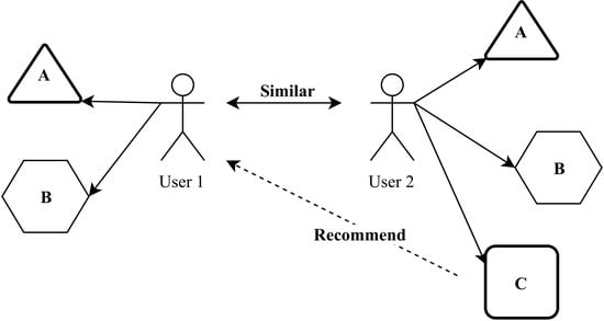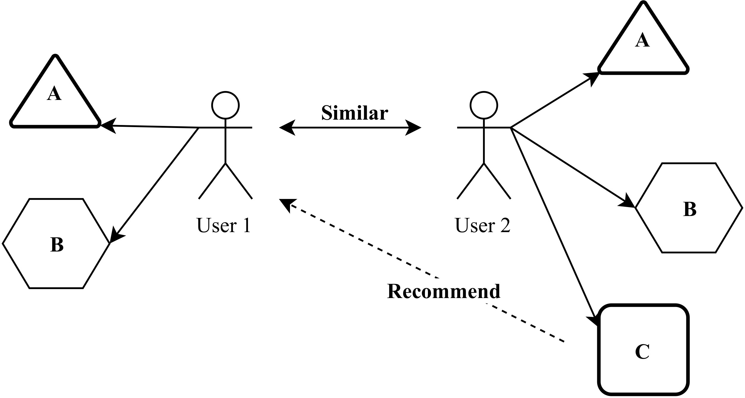Some websites using the recommender system method include yahoo.com, ebay.com, and amazon.com [1,2,3,4,5,6]. A movie recommender is an application most widely used to help customers select films from a large capacity film library. This algorithm can rank items and show users high-level items and good content to provide a movie recommended based on customer similarity. Customer similarity means collecting film ratings given by individuals based on genre or tags and then recommending films that promise to target customers based on individuals with identic tastes and preferences.

Traditional recommender systems always suffer from several inherent limits, such as poor scalability and data sparsity [7]. Several works have evolved a model-based approach to overcome this problem and provide the benefits of the effectiveness of the existing recommender system. In the literature, many model-based recommender systems were developed by partitioning algorithms, such as K-Means, and self-organizing maps (SOM) [8,9,10,11,12].

Other methods that can be used in the recommender system include the clarification method, association rules, and data grouping. The purpose of grouping is to separate users into different groups to form neighbors who are “like-minded” (closest) substitutes of searching the entire user space to increase system scalability [13]. In essence, making high-quality film recommendations with good groupings remains a challenge and exploring those following efficient grouping methods is an important issue in the recommended system situation. A very useful feature in the recommender system becomes the ability to guess user preferences and needs in analyzing user behavior or other user behaviors to produce a personalized recommender [14].

To overcome the challenges mentioned above, several methods are used to classify performance for the movie recommender system, such as K-Means algorithm [15,16,17], birch algorithm [18], mini-batch K-Means algorithm [19], mean-shift algorithm [20], affinity propagation algorithm [21], agglomerative clustering algorithm [22], and spectral clustering algorithm [23]. In this article, we develop a grouping that can be optimized with several algorithms, then obtain the best algorithm in grouping user similarities based on genre, tags, and ratings on movies with the MovieLens dataset. Then, the proposed scheme optimizes K for each cluster so that it can significantly reduce variance. To better understand this method, when we talk about variance, we are referring to mistakes. One way to calculate this error is by extracting the centroids of each group and then squaring this value to remove negative terms. Then, all of these values are added to obtain total error. To verify the quality of the recommender system, we use mean squared error (MSE), Dunn Matrix as Cluster Validity, and social network analysis (SNA). It also uses average similarity, computational time, rules of association with Apriori algorithms, and performance evaluation grouping as evaluation measures to compare the performance for recommender systems.

1.1. Prior Related Works

Zan Wang, X. Y. (2014) presented research on an improved collaborative movie recommender system to develop CF-based approaches for hybrid models to provide movie recommendations that combine dimensional reduction techniques with existing clustering algorithms. In a sparse data environment, “like-minded” selection based on the general ranking is a function of producing high-quality recommended films. Based on the MovieLens data set, an experimental evaluation approach can prove that it is capable of producing high predictive accuracy and more reliable film recommendations for existing user preferences compared to existing CF-based clustering [13]. This study also applies the clustering method to find the nearest cluster and recommends a list of movies based on similarities among users. Our recommender system dataset refers to this research by using MovieLens dataset to establish the experiments, including 100,000 ratings by 943 users on 1682 movies, with a discrete scale of 1–5. Each user has rated at least 20 movies. Then, the dataset was randomly split into training and test data at an 80% to 20% ratio. Md. Tayeb Himel, M. N. (2017) researched the weight based movie recommender system using K-Means algorithm [14]. This research uses the K-Means algorithm and explains the results. This research motivates us to use other methods as a comparison to identify the algorithm with better performance.

1.2. Problem Formulation

Information overload is a problem in information retrieval, and the recommendation system is one of the main techniques to deal with problems by advising users with appropriate and relevant items. At present, several recommendation systems have been developed for quite different domains; however, this is not appropriate enough to meet user information needs. Therefore, a high-quality recommendation system needs to be built. When designing these recommendations an appropriate method is needed. This paper investigates several appropriate clustering methods for research in developing high-quality recommendation systems with a proposed algorithm that determines similarities to define a people group to build a movie recommender system for users. Next, experiments are conducted to make performance comparisons with evaluation criteria on several clustering algorithms using the K-Means algorithm, birch algorithm, mini-batch K-Means algorithm, mean-shift algorithm, affinity propagation algorithm, agglomerative clustering algorithm, and spectral clustering algorithm. The best methods are identified to serve as a foundation to improve and analyze this movie recommender system.

1.3. Main Contributions

This study investigates several appropriate clustering methods to develop high-quality recommender systems with a proposed algorithm for finding the similarities within groups of people. Next, we conduct experiments to make comparisons on several clustering algorithms including K-Means algorithm, birch algorithm, mini-batch K-Means algorithm, mean-shift algorithm, affinity propagation algorithm, agglomerative clustering algorithm, and spectral clustering algorithm. After that, we find the best method from them as a foundation to improve and analyze this movie recommender system. We limit to using three tags and three genres because to analyze performance and get good visualization, the most stable results are three tags and three genres, before we have tried more than three but the visualization results obtained are not so good with some of the methods used in this study. We start losing the ability to visualize correctly when analyzing three or more dimensions. Then we limit it by using favorite genres and tags and more details on the algorithm comparison. The main contributions of this study are as follows:

• Performance comparison of several clustering methods to generate a movie recommender system.
• To optimize the K value in K-Means, mini-batch K-Means, birch, and agglomerative clustering algorithms.
• To verify the quality of the recommender system, we employed social network analysis (SNA). We also used the average similarity to compare performance methods and association rules with the Apriori algorithm of recommender systems.

The remainder of this paper is organized as follows. In Section 2, we present an overview of the recommender system and review the clustering algorithm and system design of the recommender system. We detail the algorithm design of the K-Means algorithm, birch algorithm, mini-batch K-Means algorithm, mean-shift algorithm, affinity propagation algorithm, agglomerative clustering algorithm, and spectral clustering algorithm. Additionally, we proposed a method to optimize K in some of the methods. This session also explains the evaluation criteria. The experiments, dataset explanation, and results are illustrated in Section 3. Evaluation results of algorithms via various test cases and discussions are shown in Section 4. Finally, Section 5 concludes this work.

2. Recommender Systems

2.1. Overview

A recommender system is a simple algorithm to provide the most relevant information for users to find patterns in the dataset. This algorithm rates the item and indicates the user who is rated high. It attempts to recommend items that best suit customer needs (in the form of products or services). A very useful feature in a recommender system is the ability to guess the preferences and user needs in analyzing user behavior or other user behavior to generate a personalized recommender [14]. The chief purpose of our system is to identify movies based on users’ viewing histories and ratings provided in the MovieLens system and datasets [24] and to use a specific algorithm to predict movies. The results are returned to the user as a recommender item with the parameters of the user. The illustration for the recommender system is presented in Figure 1, which explains similarities within people to build a movie recommendation system for users.

Figure 1 shows how two users have a similar interest in items A and B. When this occurs, the similarity index of both users will be calculated. Furthermore, the system can recommend items C to other users because the system can detect that both users have similarities in terms of the items.

2.2. System Design

In this recommender system, K-Means algorithm, birch algorithm, mini-batch K-Means algorithm, mean-shift algorithm, affinity propagation algorithm, agglomerative clustering algorithm, and spectral clustering algorithm are used to determine the best performing algorithms in movie recommendations based on optimized K values. After applying several algorithms, all spaces are searched to obtain the user nearest neighbor in the same cluster and Top-N List of recommender movies. Figure 2 shows an overview of the flow of seven existing algorithms.

2.3. Clustering Algorithm

Clustering is an analytical method that was used as early as 1939 by Tryon, R. C [25]. Clustering was first used in psychology and then rapidly expanded to other fields. Since the explosion of the amount of information available on the internet, many efforts have been made to reduce the problem of information overload. This overload can be resolved by using a clustering method. Clustering is a classification of the same objects from different groups with partitions using existing data into a new group, and each group of data is identified with a certain degree of distance. In cluster analysis, there is also a contrast between parametric and nonparametric approaches [26]. Data clustering is a technique commonly used in various fields, such as data mining, pattern recognition, image analyze, and artificial intelligence. Data clustering is employed to reduce a large amount of data by providing the categories or classifying the data that have a high degree of similarity.

2.3.1. K-Means Clustering Algorithm and Optimize K Number Cluster

K-Means clustering is a method that automatically divides datasets into k groups [27]. Results selected the initial central cluster k to be iteratively refined by being assigned to the nearest central cluster. Each center of the $C_j$ cluster is updated to an average sample of its constituents.

K-Means is used to group approaches given its simplicity, efficiency, and flexibility in calculations especially considering a large amount of data. K-Means calculate the cluster center in assigning objects to the closest cluster based on distance. When the midpoint does not change, the clustering algorithm seeks convergence. However, K-Means lacks the ability to choose the right initial seeds and could cause classification inaccuracies. Selecting a random starting seed can produce a locally good solution that is quite inferior to finding the direct K value. The various initial seeds that run on the same dataset might deliver different partition results. Given a set of objects $(x_1,x_2,\cdots ,x_n)$, where each object is an m-dimensional vector, the K-Means algorithm aims at separating these objects to form k groups automatically. Algorithm 1 provides the K-Means procedure.

Algorithm 1K-Means algorithm and optimize k number cluster

Intput:  Selecting dataset and using dataset by each user avg rating with favorite genre/tags; Output:  Finishing with release Top-N list of recommendation movie for similarity user;  1: functionK-Means()  2:        Choosing k initial cluster centers  3:          $C_j,j=1,2,3\cdots ,k$;  4:     Each $x_i$ is assigned to its closest cluster  5:        center based on the distance metric  6:     $J={\sum }_{j=1}^k{\sum }_{i\in C_{temp}}\left|\right|x_i-M_j{\left|\right|}^2$,  7:        where $M_j$ denotes the mean of data points  8:        in $C_{temp}$;  9:     Choosing the right K number of Clusters; 10:     clustering the user’s rate movies; 11:     Finding the nearest node to search similarity with 12:        user with Euclidean distance; 13:     if there is not change then 14:         The algorithm has converged and clustering task 15:         is ended, also recalculate the M of K clusters 16:         as the new cluster centers and go to; 17:     end if 18: end function

Optimize K Number Cluster

To overcome the limitations above, we optimized K to choose the correct number of K clusters. Choosing the best number of K clusters is the key point of the K-Means algorithm. To find K, we calculate the clustering error with mean squared error (MSE) and silhouette score. First, we select a dataset and choose the range of k values to test. Then, we define the function to calculate the clustered errors and error values for all k values. Finally, we plot each value of k with the silhouette score at that value. A detailed explanation of mean squared error (MSE) and silhouette score is provided in [28,29].

(1) Silhouette Score to determine the K number cluster. The silhouette was first introduced by Peter J. Rousseeuw in [30] in 1986. This is a method of interpretation and validation for clear data clusters. This technique provides a graphical representation of how well each object fits inside the group. The silhouette value for an attribute is given by the equation below:

$$\begin{array}{c}\hfill S_i=\frac{a\left(i\right)·b\left(i\right)}{max\left\{a\left(i\right),b\left(i\right)\right\}},\end{array}$$

(1)

where $a\left(i\right)$ is the average dissimilarity of data point i with other data within the one cluster. Here, $b\left(i\right)$ is the minimum average dissimilarity of data point i with any other cluster in which i is not inside member a.

2.3.2. Birch Clustering Algorithm

Balanced iterative reducing and clustering using hierarchies (birch clustering) uses a hierarchical data structure that calls CF-tree for increment and dynamically clusters data points [31]. The birch algorithm uses an input set of data points N, which is represented as a vector of real value and the desired number of cluster K. The first phase builds a CF-tree from a data point. This can be defined with given a set of N d-dimensional data points, and the clustering feature (CF) of the set is used to establish the triple- $CF=(N,LS,SS)$, where

$$\begin{array}{c}\hfill \overrightarrow{LS}=\sum _{i=1}^N\overrightarrow{x_i},\end{array}$$

(2)

is the linear sum and

$$\begin{array}{c}\hfill \overrightarrow{SS}=\sum _{i=1}^N\overrightarrow{{\left(x_i\right)}^2},\end{array}$$

(3)

is the sum of the data points.

Clustering features are organized on a CF-tree, a height-balanced tree within two parameters, including branching factor B and threshold T. Each non-leaf node contains most B entries inside the form [$C{F}_i$, child${}_i$], in which child i is one pointer to its i the child node and $C{F}_i$ is the clustering feature representing the associated subcluster.

2.3.3. Mini-Batch K-Means Clustering

The algorithm Mini-batch K-Means was developed as a modification of the K-Means algorithm. It uses mini-batch to reduce time in very complex and large-scale calculations of datasets. The efforts to optimize grouping results could be used with this method. Mini-batch K-Means are randomly used as input, which is a subset of the entire dataset. Mini-batch K-Means is faster than K-Means and is usually used for large datasets. For dataset $T=\{x1,x2,\cdots ,x_n\},x_i\in R^{m·n}$, $x_i$ represents a network record with an n-dimensional real vector. In addition, m indicates the number of records inside the dataset T. The objective of the clustering problem is to uncover the set C of cluster centers $c\in R^{m·n}$ to minimize the dataset T of records $c\in R^{m·n}$ in function [32]. In contrast to K-Means, mini-batch K-Means randomly selects a subset of records from the dataset. Mini-batch K-Means greatly reduces the clustering time and the convergence time. The sum of squared distances is computed in one cluster as follows:

$$\begin{array}{c}\hfill \min \sum _{x\in T}\left|\right|f(C,x)-{x\left|\right|}^2,\end{array}$$

(4)

where $f(C,x)$ returns the closest of cluster center $c\in C$ to record x, and $\left|C\right|=K$ and K is the number of clusters to obtain.

2.3.4. Mean-Shift Clustering

The mean-shift algorithm is proposed as a method for cluster analysis [33]. However, given that the mean-shift determines the gradient ascent, the convergence of the process needs verification and its relation with similar algorithms needs clarification. The mean-shift algorithm is part of a nonparametric grouping technique that does not require prior knowledge of the number of clusters and does not constrain the shape of the clusters. Mean-shift clustering is used to discover blobs in a smooth density of samples, which works by updating the candidates for centroids to be the mean points within a given region. These candidates are then filtered in a postprocessing stage to eliminate near-duplicates to form the final set of centroids. Given a candidate centroid $x_i$ followed by iteration t, the candidate is updated by the following equation:

$$\begin{array}{c}\hfill x_i^{t+1}=m\left(x_i^t\right),\end{array}$$

(5)

where $N\left(x_i\right)$ is the neighborhood of samples within a given distance around $x_i$ and m is the mean-shift vector for each centroid that points against a region of the maximum increase in the density of points. This is computed using the following equation:

$$\begin{array}{c}\hfill m\left(x_i\right)=\frac{{\sum }_{x_j\in N\left(x_i\right)}K(x_j-x_i)x_j}{{\sum }_{x_j\in N\left(x_i\right)}K(x_j-x_i)}.\end{array}$$

(6)

The algorithm can automatically determine the number of clusters, using bandwidth parameters. This information can determine the size of the region to search through. This algorithm is unreachable because it requires several close neighbor searches during its execution.

2.3.5. Affinity Propagation Clustering

In the affinity propagation method all data points are considered as possible exemplars. It exchanges real-values between exemplars until high-quality exemplars and corresponding clusters are not provided. The particular messages are further updated based on a simple formula that ratiocinates a sum-product. At any selected point in time, the magnitude in each message represents the current affinity that one point has for choosing another data point as its exemplar, hence the name “affinity propagation” [34]. The messages sent between points belong to one of the two categories. The accumulated evidence $r(i,k)$ of sample k should be the exemplar for sample i. In addition, regarding availability $a(i,k)$, the accumulated indicates that sample i should choose sample k to be an exemplar. The exemplar chosen by samples is similar enough to many samples that are representative of themselves. The responsibility of a sample k to be the exemplar of sample i is given by the following formula:

$$\begin{array}{c}\hfill r(i,k)\leftarrow s(i,k)-max[a(i,k^{\prime })+s(i,k^{\prime })\forall k^{\prime }\ne k].\end{array}$$

(7)

The similarity between samples i and $k,s(i,k)$ is assessed. The availability of sample k to be an exemplar to sample i is given by the following formula:

$$\begin{array}{c}\hfill a(i,k)\leftarrow min[0,r(k,k)+\sum _{i^{\prime }s,t,i^{\prime }\in \{i,k\}}r(i^{\prime },k)].\end{array}$$

(8)

We define a cluster with update $r(i,k)$ and $a(i,k)$. All the values for r and a were set to zero and each iterate is calculated until convergence is found. To avoid numerical oscillations, the iteration process requires the damping factor $\gamma$ as follows:

$$\begin{array}{c}\hfill r_{t+1}(i,k)=\lambda ·r_t(i,k)+(1+\lambda )·r_{t+1}(i,k),\end{array}$$

(9)

$$\begin{array}{c}\hfill a_{t+1}(i,k)=\lambda ·a_t(i,k)+(1+\lambda )·a_{t+1}(i,k).\end{array}$$

(10)

2.3.6. Agglomerative Clustering

Agglomerative clustering can scale large numbers of samples when used together with the connectivity matrix and all possible merges are considered at each step. Ward’s method is one of the agglomerative clustering methods based on a classical sum-of-squares criterion, producing groups that minimize within-group dispersion at each binary fusion. This method uses Euclidean distance as the distance metric.

$$\begin{array}{c}\hfill \left|\right|a-{b\left|\right|}_2=\sqrt{\sum _i{(a_i-b_i)}^2}.\end{array}$$

(11)

2.3.7. Spectral Clustering

Spectral clustering uses information from the eigenvalue (spectrum) of a special matrix that will be built from a graph or data set. This matrix will be built and interpret its spectrum using eigenvectors to assign data to clusters. An eigenvector is an important object of linear algebra and helps illustrate the dynamics of the system represented by the matrix. Specific grouping uses the concept of eigenvalues and eigenvectors.

$$\begin{array}{c}\hfill L=D^{-1/2}·A{D}^{-1/2}.\end{array}$$

(12)

Its closest cluster center is assigned based on the distance metric. The affinity matrix is formed, and the diagonal matrix is defined. The matrix is formed and the normalized Laplacian matrix and eigenvectors are computed.

2.4. Evaluation Criteria

We utilized the training data to develop the offline model, and the remaining data are used to analyze and provide the movie recommendation. To verify the quality of the recommender system, we employed the mean squared error (MSE), social network analysis (SNA), Dunn Matrix as cluster validity indices, and evaluation measures with average similarity, computational time, association rule with Apriori algorithm, and clustering performance evaluation. The following is verified and evaluated.

2.4.1. Mean Squared Error

Mean squared error (MSE) is used to facilitate training and some overall error measure is often used as a performance metric or an objective function [35].

$$\begin{array}{c}\hfill \mathrm{MSE}=\frac{1}{M}·\frac{1}{N}\sum _{m=1}^M\sum _{j=1}^N{\left(d_{mj}-y_{mj}\right)}^2,\end{array}$$

(13)

where $d_{mj}$ and $y_{mj}$ represent the desired (target) value and output at the m the node for the j the training pattern respectively, M is the number of output nodes, and N is the number of the training patterns. The purpose of training is to detect the set of weights that minimize the objective function.

Mean squared error (MSE) is very clever in providing information about this artificially built model. By minimizing the mean squared error (MSE) value, the variant model is minimized. This can provide relatively consistent results as input data compared to models with large variants (large mean squared error (MSE)).

2.4.2. Clustering Validity Indices: Dunn Matrix

The Dunn index (DI) is a metric for evaluating clustering algorithms with internal evaluation schemes, with results being based on the cluster data itself. Dunn’s index is the ratio of within and between cluster separation (Malay K. Pakhira, S. B., 2004). Similar to all other indices, the purpose of the Dunn index is to identify a set of compact clusters with small variants between cluster members, that are well separated, and within which the average cluster differs significantly compared to the cluster variants.

The higher the Dunn index value is, the better the grouping. The number of clusters maximizing the Dunn index will be taken as the optimal number of clusters k. It also has several shortcomings. As the number of clusters and data dimensionality increase, the cost of computing also increases. The Dunn index for c number of clusters is defined as follows:

$$\begin{array}{c}\hfill \mathrm{Dunn}\mathrm{index}(U)=\underset{1\le i\le c}{min}\left\{\underset{1\le i\le c}{min}\left\{\frac{\delta (X_i,X_j)}{\underset{1\le i\le c}{max}\{\Delta \left(X_k\right)\}}\right\}\right\}.\end{array}$$

(14)

2.4.3. Social Network Analysis

To understand relations between one user and another user in clustering, we used social network analysis (SNA). Social network analysis (SNA) is a collection of relational methods used to understand and identify relationships between actors systematically [36], which is widely utilized in the system to determine the level of relation or similarity between users or actors. User relationships in the clustering could be known through centrality. There are three general centrality measurements, as reported below [35]:

Degree

Degree is the number of relations. An actor with the most relationships is the most important actor. To search density, the most varied grouping with similarity users in one cluster can be calculated using the following equation:

$$\begin{array}{c}\hfill C_D=d\left(n_i\right)=\sum _j{x}_{ij},\end{array}$$

(15)

where $C_D$ is centrality degree, $d\left(n_i\right)$ is degree of node i, and $X_{ij}$ is edge $i-j$.

Closeness

Closeness is the proximity of actors with other actors. The actor is critical of its close relation to other actors. Both clusters have a high linkage relationship. It can be calculated using the following equation:

$$\begin{array}{c}\hfill C_c\left(n_i\right)={\left[\sum _{j=1}^{g}d(n_i,n_j)\right]}^{-1},\end{array}$$

(16)

where $C_c\left(n_i\right)$ is centrality closeness of node I and $d(n_i,n_j)$ is edge $i-j$

$$\begin{array}{c}\hfill C_c^{\prime }=\left(n_i\right)=\left(C_c\left(n_i\right)\right)·(g-1).\end{array}$$

(17)

Betweeness

Betweenness is used to calculate the number of shortest paths between actors j and k where actor i is located. The shortest distance has the highest relation between clusters. It can be calculated using the following equation:

$$\begin{array}{c}\hfill C_B\left(n_i\right)=\sum _{j<k}\frac{g_{jk}·\left(n_i\right)}{g_{jk}}\end{array}$$

(18)

where $C_B\left(n_i\right)$ is betweenness actor centrality (node) $i,CHF\left(n_i\right)$ is the number of actors path where i is, and $CHF$ is the number of the path that connects actors j and k.

2.4.4. Average Similarity

Average similarity represents the similarity between two clusters. High similarity represents a benchmark for how many clusters are clustering. Cosine similarity measures the similarity between two nonzero vectors by taking the cosine of the angle from between vectors that intervene in their dot product space [37]. The measure is independent of vector length, which makes it a measure typically used for high-dimensional spaces. The cosine of two nonzero vectors can be derived using the Euclidean dot product formula:

$$\begin{array}{c}\hfill A·B=\left|\right|A\left|\right|·\left|\right|B\left|\right|·cos\left(\theta \right)\end{array}$$

(19)

Given two vectors of attributes, A and B, the cosine similarity, $cos\theta$, is represented using a dot product and magnitude as follows:

$$\begin{array}{cc}\hfill \mathrm{similarity}& =cos\left(\theta \right)=\frac{A·B}{\left|\right|A\left|\right|·\left|\right|B\left|\right|}\hfill \\ \hfill & =\frac{{\sum }_{i=1}^n{A}_i·B_i}{\sqrt{{\sum }_i=1^n{A}_i^2}·\sqrt{{\sum }_{i=1}^n{B}_1^2}}.\hfill \end{array}$$

(20)

2.4.5. Computational Time

Computational time is the run time, which is the length of time that is needed to perform the computation process in a program. In this case, the computation time (CT) is calculated as the end time(e) of the algorithm program minus the start time(s) to compare the time performance required. Computational time, in this case, is given by the following formula:

$$\begin{array}{c}\hfill CT=e-s.\end{array}$$

(21)

2.4.6. Association Rule: Apriori Algorithm

Association rule mining is a technique for identifying the fundamental relationships between various items. Profits will be gained from the sale of more items. From the user’s transaction data set, rules can be made for customer purchasing trends. Based on the selected movie and customer tastes, it can produce recommendations using the association rules mining technique. Association rule mining is used to find correlations between customers and products [38]. The mining technique of multidimensional association rules is used to identify the most accurate recommendation and assess the movie recommender list. Preprocessing techniques are also used for the rules of association with Apriori algorithms. Apriori algorithms can be used so that computers can learn the rules of the association to identify patterns of relationships between one or more items in a dataset. Thus, by using association rules and clustering techniques, we can create an efficient recommendation system that provides recommendations in a shorter time. For example, if the user chooses movie A, and movie B has similarities with movie A, then the user has a tendency to choose movie B that has similarities with movie A and movie C that has similarities with movie B.

There are three major components of the Apriori algorithm, including Support, Confidence, and Lift. Item A is represented by X, and Item B is represented by Y, which are described below.

Support

The term support represents the default popularity of an item. It is calculated based on the division between the number of transactions containing a selected item and the total number of transactions. Here, suppose that we want to find support for item B. This is calculated using the following formula:

$$\begin{array}{cc}\hfill \mathrm{Support}& \left(\right\{X\}\to \{Y\left\}\right)\hfill \\ \hfill & =\frac{\mathrm{Transactions}\mathrm{containing}\mathrm{both}X\mathrm{and}Y}{\mathrm{Total}\mathrm{number}\mathrm{of}\mathrm{transactions}}.\hfill \end{array}$$

(22)

Confidence

Confidence refers to the possibility that item B is also purchased if item A is purchased. This can be calculated by finding the number of transactions where A and B were bought together and then divided by the total number of transactions where A was purchased. Mathematically, this relationship is shown below:

$$\begin{array}{cc}\hfill \mathrm{Confidence}& \left(\right\{X\}\to \{Y\left\}\right)\hfill \\ \hfill & =\frac{\mathrm{Transactions}\mathrm{containing}\mathrm{both}X\mathrm{and}Y}{\mathrm{Transactions}\mathrm{containing}X}.\hfill \end{array}$$

(23)

Lift

Lift(A → B) refers to the increase in sales ratio B when A is sold. Lift(A → B) can be calculated by dividing Confidence (A → B) divided by Support (B). Mathematically this relationship is shown below:

$$\begin{array}{cc}\hfill \mathrm{Lift}& \left(\right\{X\}\to \{Y\left\}\right)\hfill \\ \hfill & =\frac{\frac{\mathrm{Transactions}\mathrm{containing}\mathrm{both}X\mathrm{and}Y}{\mathrm{Transaction}\mathrm{containing}X}}{\mathrm{Fraction}\mathrm{of}\mathrm{transactions}\mathrm{containing}Y}.\hfill \end{array}$$

(24)

2.4.7. Clustering Performance Evaluation

In this section, the seven clustering algorithm indices that have been used in this article to evaluate the partition obtained by the above three techniques for different values of index are described [39].

Silhouette Coefficient

If the truth label is unknown, the evaluation must be performed using the model itself. This is the case for the silhouette coefficient where the higher score is connected to a model with a better group. We defined the coefficient for each sample. This contains two scores. Specifically, a represents the distance between sample A and all other points in the same class, and b represents the distance between sample B and other points in the next nearest cluster. The distance metric could be calculated using Euclidean distance or the Manhattan distance. The coefficient s for a single sample is then retrieved as follows:

$$\begin{array}{c}\hfill s=\frac{b-a}{max(a,b)}.\end{array}$$

(25)

Calinski-Harabaz Index

If the ground truth labels are not known, the Calinski-Harabasz index can be used to evaluate the model. A higher Calinski-Harabasz score relates to a model with better clusters assignments. For k clusters, the Calinski-Harabasz score is given as the ratio of the between-clusters dispersion mean and the within-cluster dispersion:

$$\begin{array}{c}\hfill s\left(k\right)=\frac{Tr\left(B_k\right)}{TR\left(w_k\right)}\times \frac{N-k}{k-1},\end{array}$$

(26)

where $B_k$ is the between group dispersion matrix, and $W_k$ is the within-cluster dispersion matrix, which is defined as follows:

$$\begin{array}{cc}\hfill W_k& =\sum _{q=1}^k\sum _{x\in c_q}(x-c_q)·{(x-c_q)}^T,\hfill \end{array}$$

(27)

$$\begin{array}{cc}\hfill B_k& =\sum _q{n}_q·(c_q-c)·{(c_q-c)}^T,\hfill \end{array}$$

(28)

where the N entity is the number of points in data, $C_q$ is the set of points in cluster $e_q$, $C_g$ is the center of cluster q, c is the set center of E, and $n_q$ is the number of points inside cluster q.

Davies–Bouldin Index

Similar to the Calinski-Harabaz Index case when the ground truth labels are not known, the Davies Bouldin index can be used for the model evaluation. Here, a lower index is related to a model with better disjunction between the clusters. A simple choice to construct $R_{ij}$ is nonnegative and symmetric as follows:

$$\begin{array}{c}\hfill R_{ij}=\frac{s_i\to s_j}{d_{ij}}.\end{array}$$

(29)

The index is defined as the average similarity between each cluster $C_i$ for $i=1$, k and its most similar cluster $C_j$. Regarding the context inside the index, the similarity is defined as a measure $R_{ij}$ that trades the $s_i$, the average distance between each point of cluster i and the centroid of that cluster. It is also defined as the distance between cluster centroids i and j. Then the Davies–Bouldin Index is established as follows:

$$\begin{array}{c}\hfill DB=\frac{1}{k}\sum _{i=n}^k\underset{i\ne j}{max}{R}_{ij}.\end{array}$$

(30)

3. Experiment Results

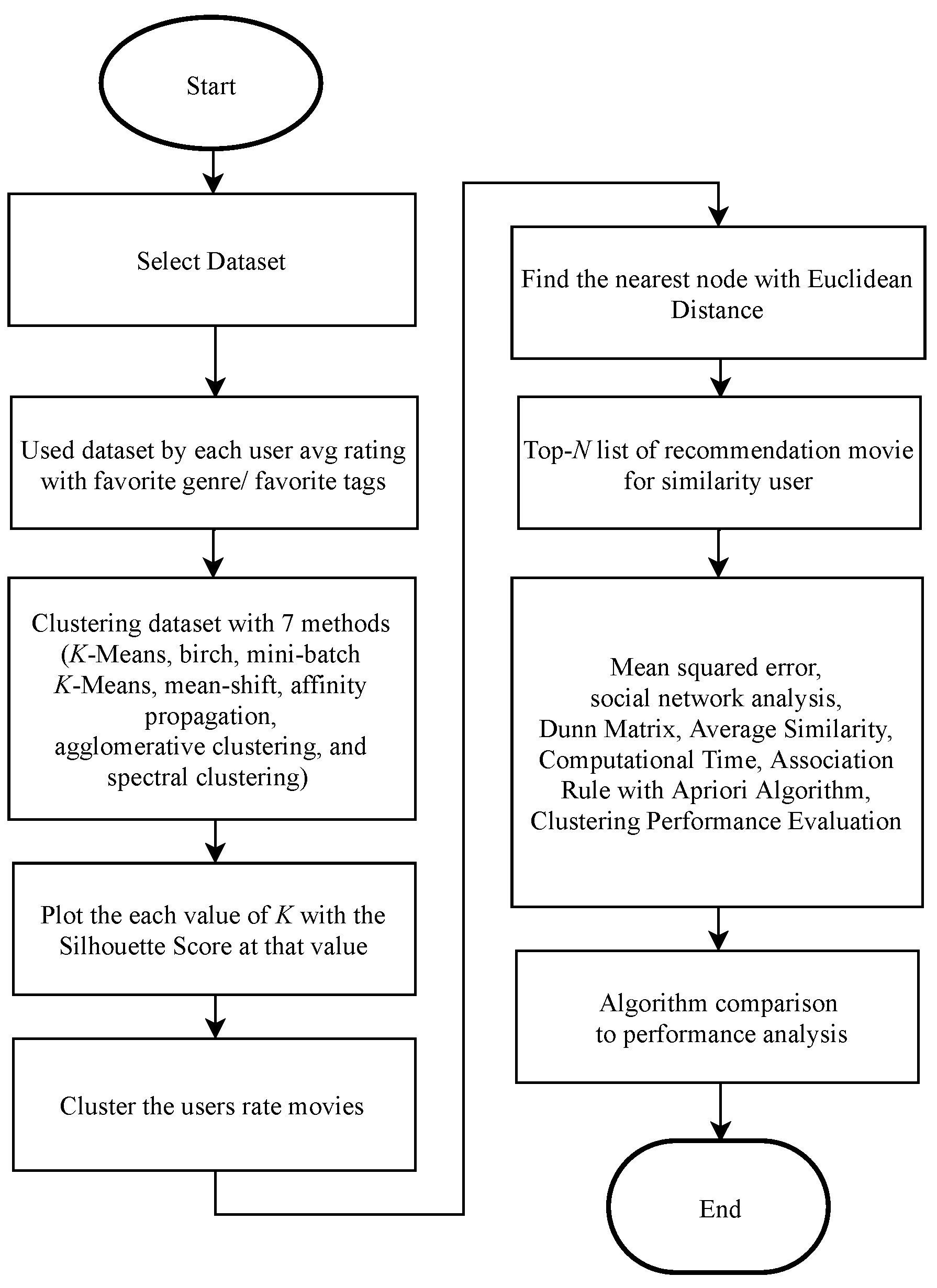
In this part, the experimental design and empirical result of the proposed movie recommender algorithm via K-Means, birch, mini-batch K-Means, mean-shift, affinity propagation, agglomerative clustering, and spectral clustering technique are presented. To verify the quality of the recommender system, the mean squared error (MSE), Dunn Matrix as cluster validity indices, and social network analysis (SNA) are used. Average similarity, computational time, association rule with Apriori algorithm, and clustering performance evaluation are used as evaluation measures. Finally, the results are analyzed and discussed. These experiments were performed on Intel(R) Core(TM) i5-2400 CPU @ 3.10 GHz, 8.0 GB RAM computer and run Python 3 with Jupyter Notebook 5.7.8 version to simulate the algorithm.

3.1. Dataset

We use the MovieLens dataset to conduct an experiment and this dataset is also available online. The dataset is a stable benchmark dataset within 20 million ratings and 465,000 tag applications applied to 27,000 movies, including 19 genres, by 138,000 users. The tag data with 12 million relevance scores are incorporated across 1100 tags. Datasets are determined using a discrete scale of 1–5. We limit the use of clustering based on three genres and three tags to analyze the performance and get a good visualization. High dimensional could not be handled properly, so the visualization results were not suitable when using all tags and genres. Afterwards the dataset was randomly split into training and test data with a ratio of 80%/20%. The goal is to obtain similarities within groups of people to build a movie recommending system for users. Then, we analyze a dataset from MovieLens user ratings to examine the characteristics people share with regard to movie taste and use this information to rate the movie.

3.2. Algorithm Clustering Result

We try to establish different clustering algorithms using K-Means, birch, mini-batch K-Means, mean-shift, affinity propagation, agglomerative clustering, and spectral clustering techniques to discover similarities within groups of people to develop a movie recommendation system for users. Then, clustering based on three genres and three tags is used to analyze the performance, obtain good visualization, and sort movie ratings from high to less by assigning the dataset using a discrete scale of 1–5. Then, to overcome the above limitations, K was optimized to select the right K number of clusters. Euclidean distance was also used to find the closest neighbor or user in the cluster. Finally, this study recommends the list-N of movie list based on user similarity. 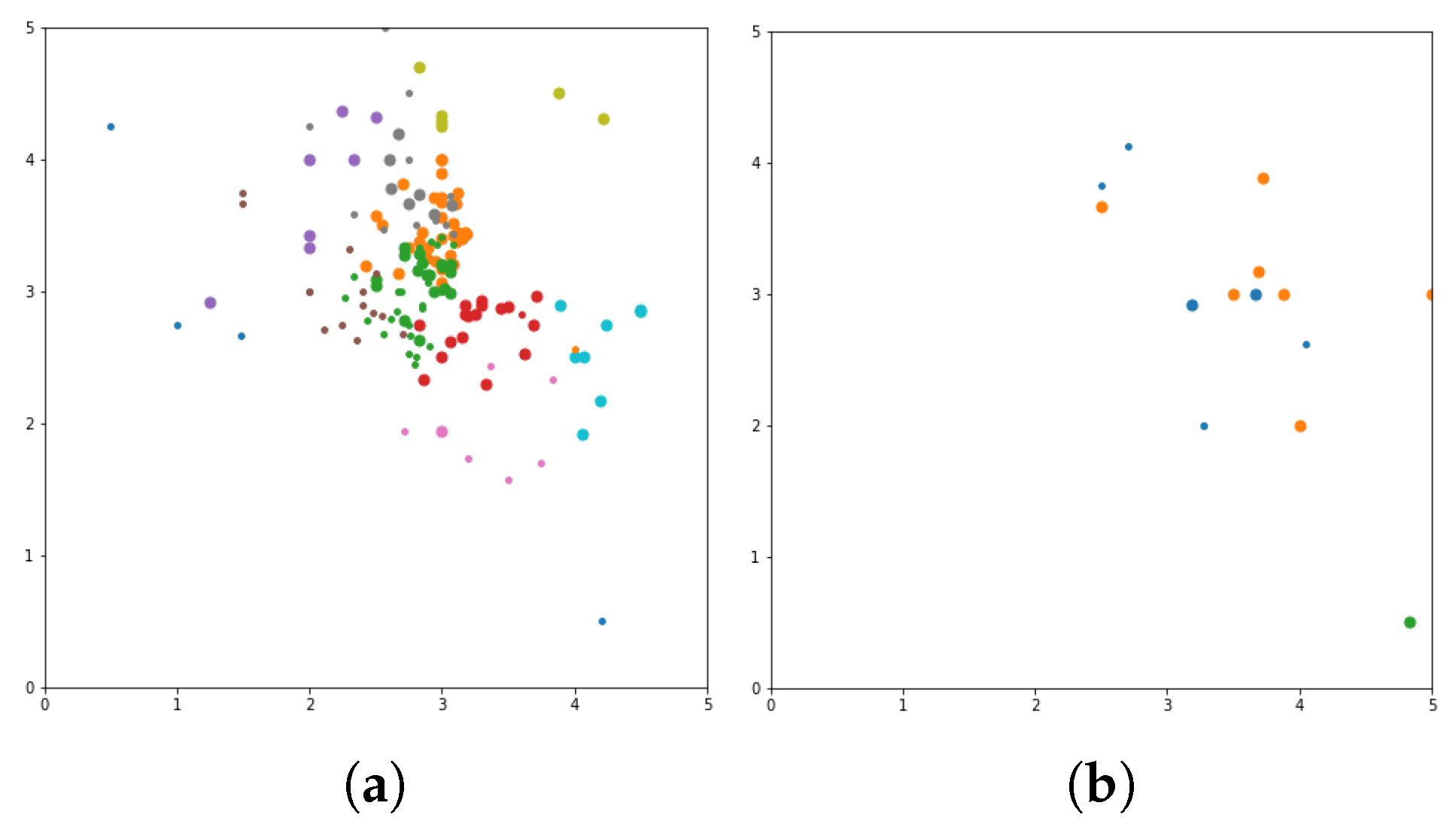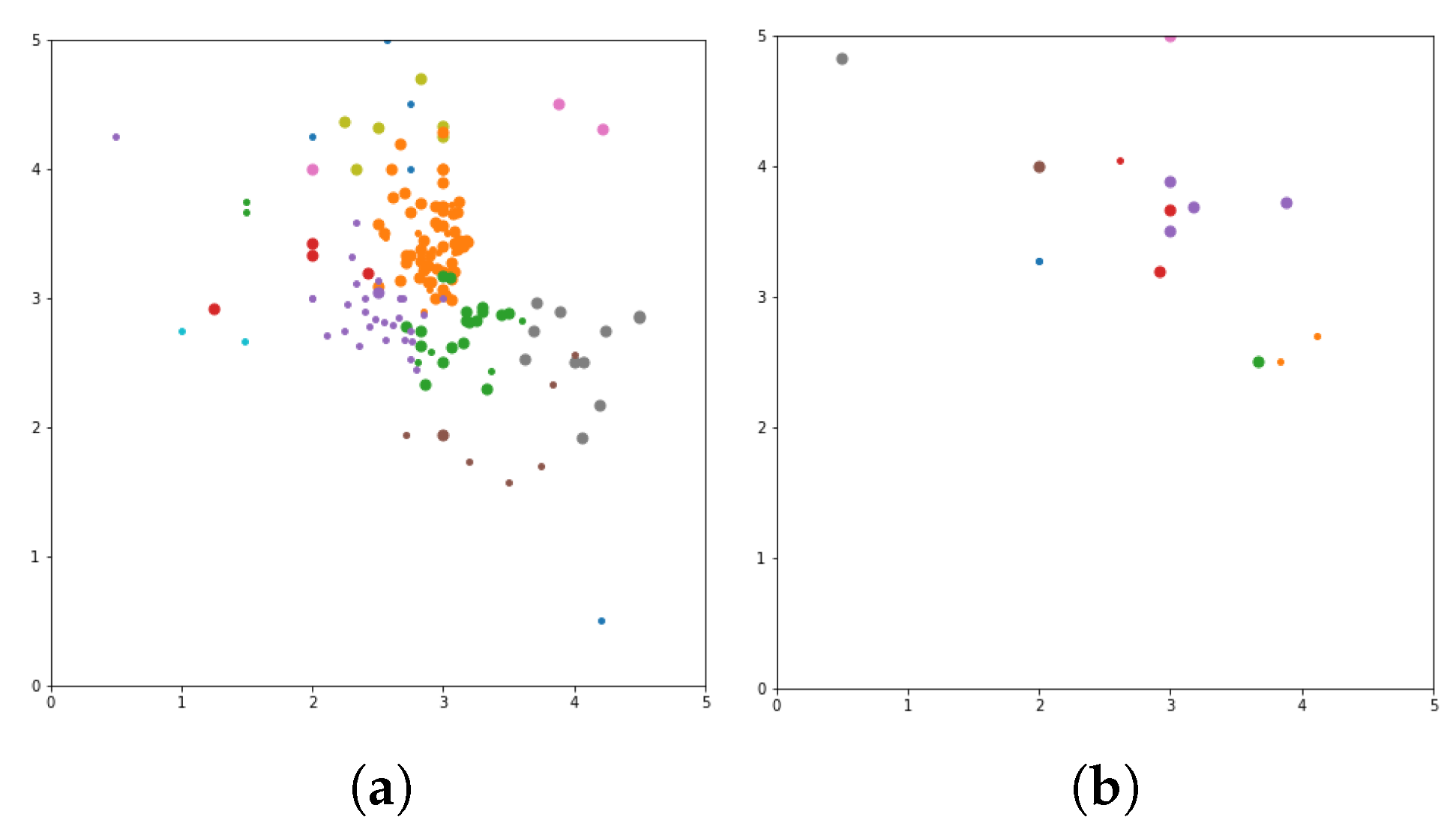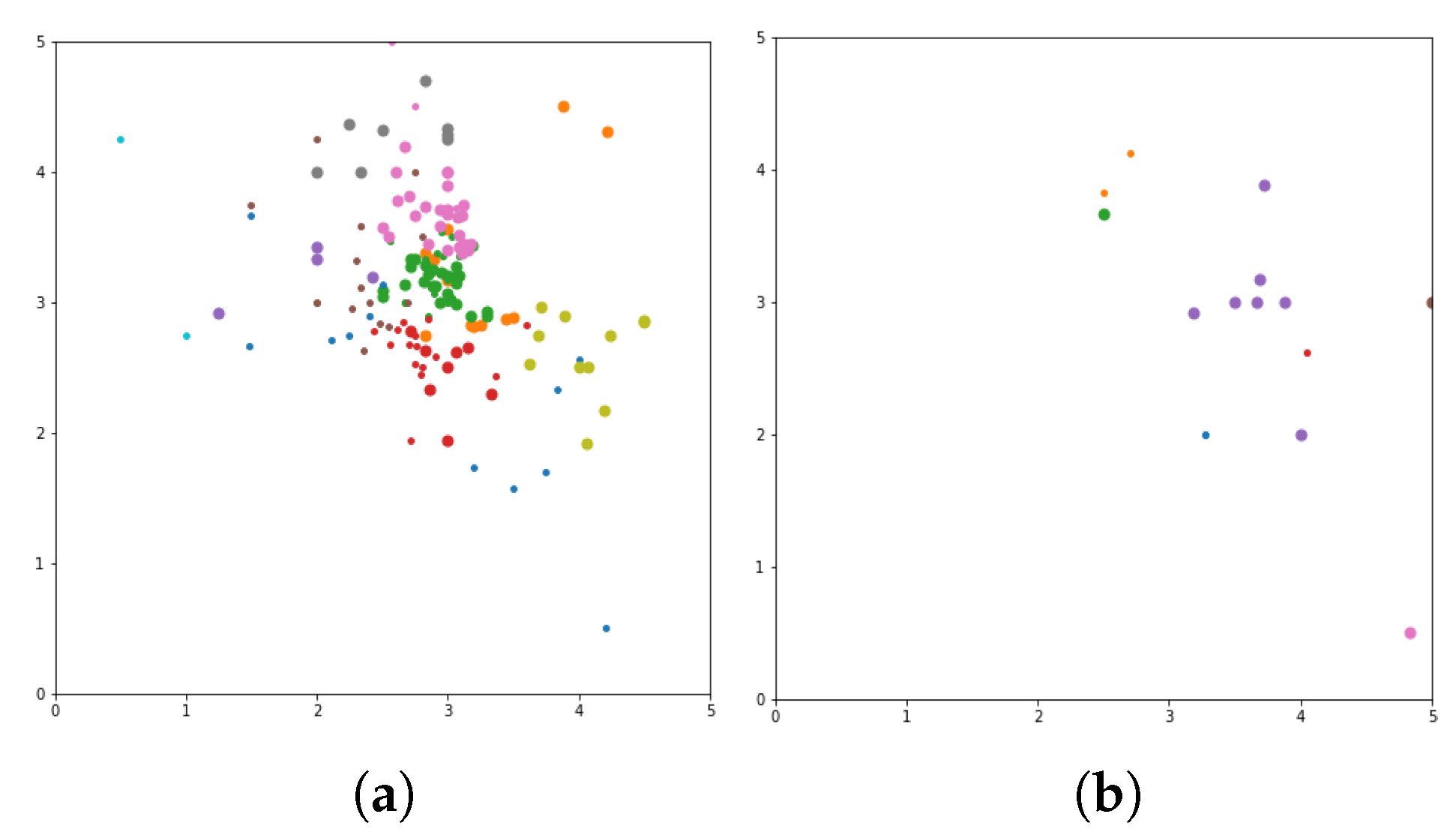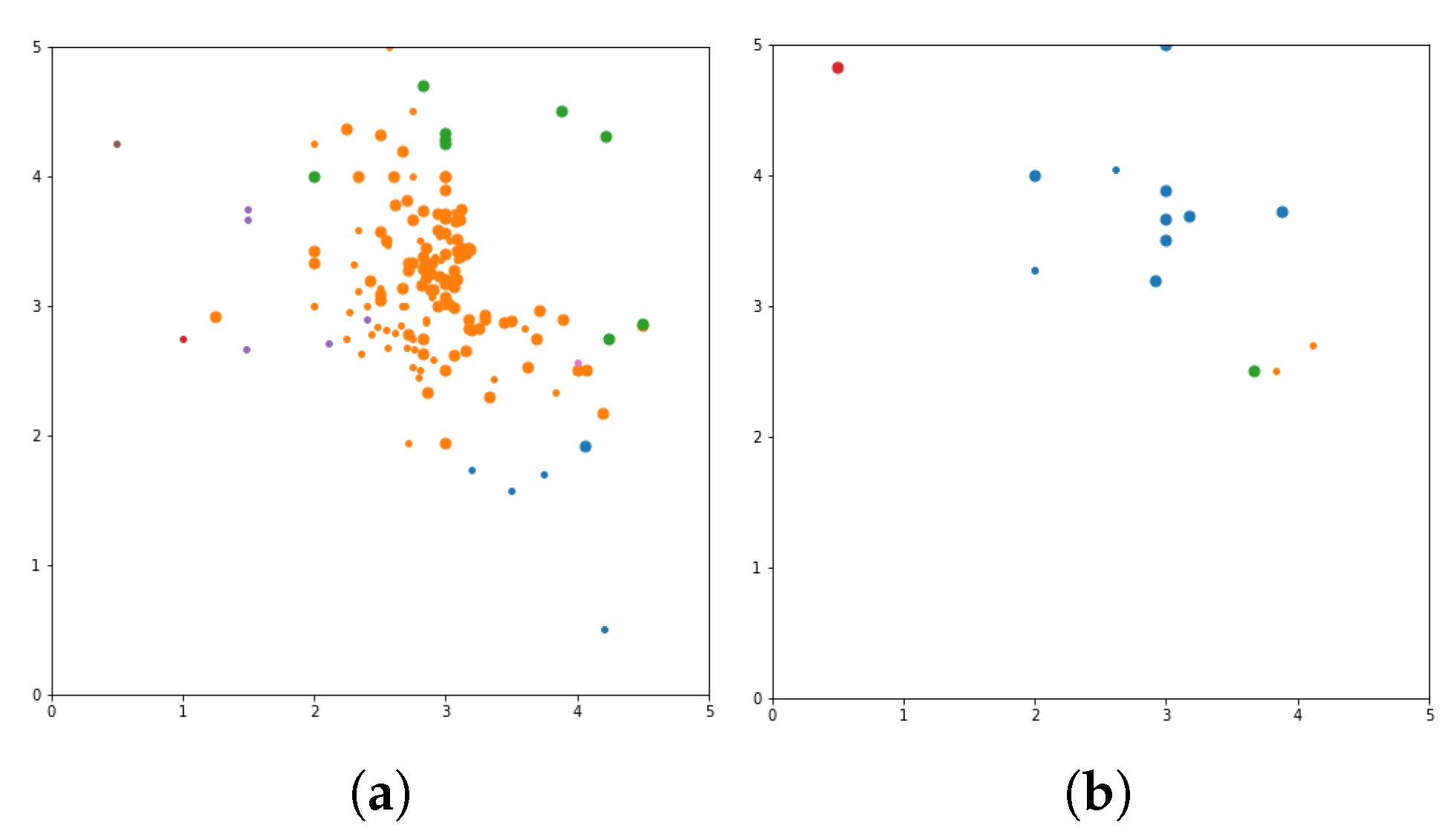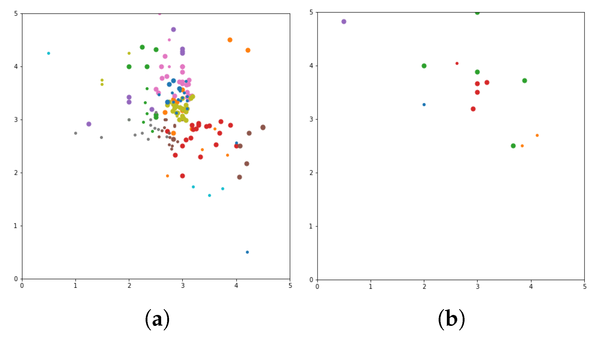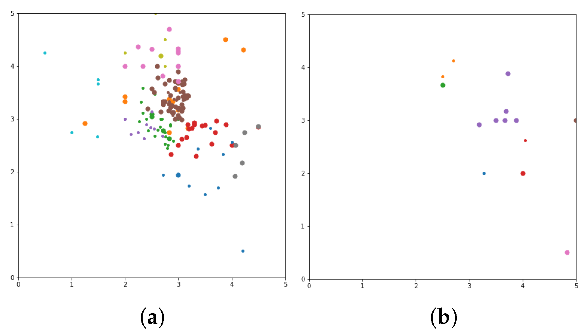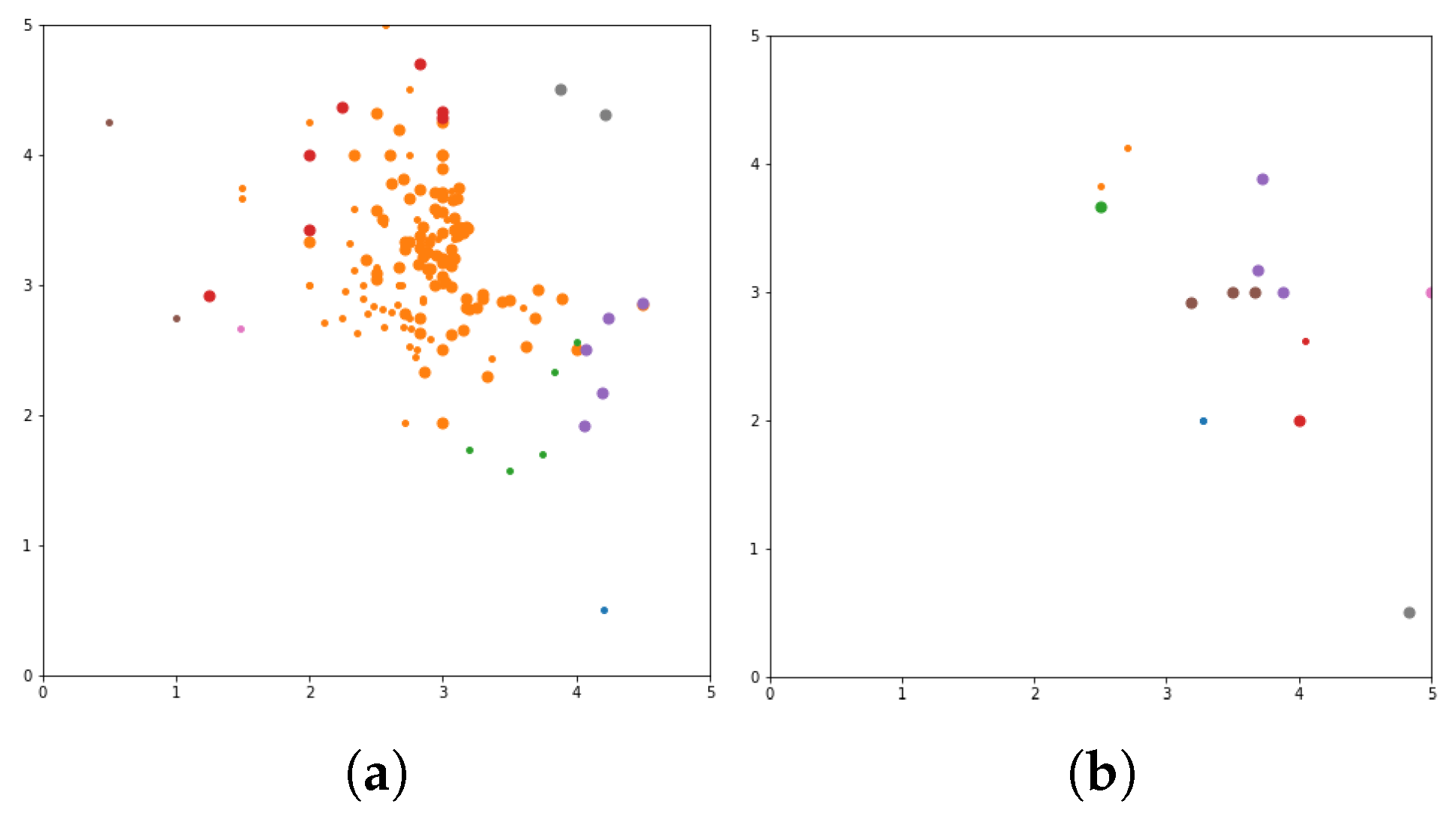The visualization clustering results for seven different algorithms are presented (see Figure 3, Figure 4, Figure 5, Figure 6, Figure 7, Figure 8 and Figure 9). In these figures the X-axis for the first subfigures is the average romance rating, and the Y-axis is the average sci-fi rating. For the second subfigures, the X-axis is the average fantasy rating, and average funny rating is reported on the Y-axis.

To obtain a more delimited subset of people to study, grouping is performed to exclusively obtain ratings from those who like either romance or science fiction movies. X and Y-axes are romance and sci-fi ratings, respectively. In addition, the size of the dot represents the ratings of the adventure movies. The bigger the dot, the higher the adventure rating. The addition of the adventure genre significantly alters the clustering. The Top N-Movies lists several clustering algorithms with K-Means genre n cluster = 12, K-Means tag n cluster = 7, birch genre n cluster = 12, birch tags n cluster = 12, MiniBatch-K-Means genre n cluster = 12, MiniBatch-K-Means tags n clusters = 7, mean-shift genre, mean-shift tags, affinity propagation genre, affinity propagation tags, agglomerative clustering genre n cluster = 12, agglomerative clustering tag n cluster = 7, spectral clustering genre, spectral clustering tags are reported below.

Considering a subset of users and discovering what their favorite genre was, we define a function that would calculate each user’s average rating for all romance movies, science fiction movies, and adventure movies. To obtain a more delimited subset of people to study, we biased our grouping to exclusively obtain ratings from those users who who like either romance or science fiction movies. We used the x and y-axes of the romance and sci-fi ratings. In addition, the size of the dot represents the ratings of the adventure movies (the bigger the dot, the higher the adventure rating). The addition of the adventure genre significantly affects the clusters. The more data added to our model, the more similar the preferences of each group are. 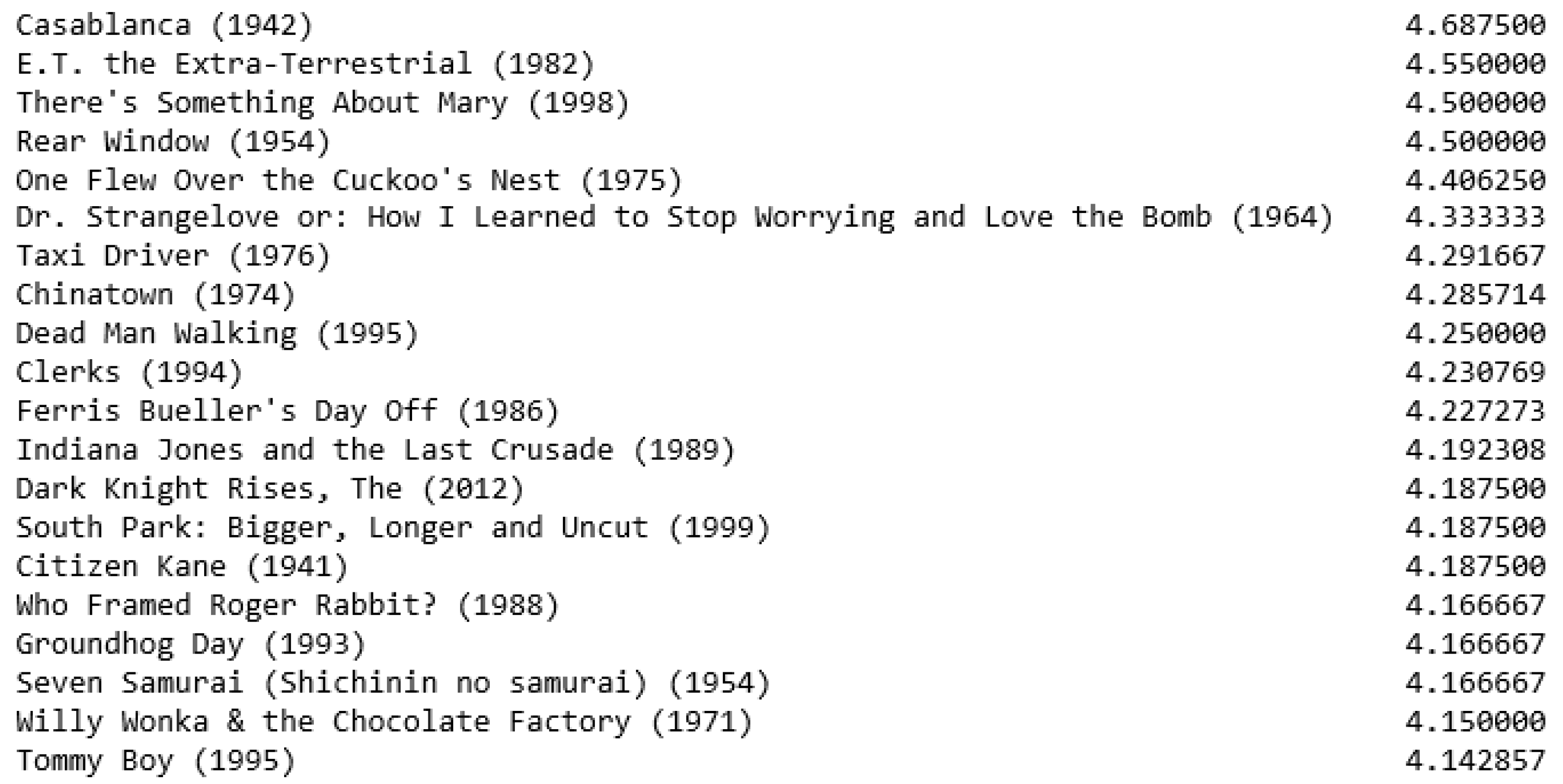The final version is Top list of N of movies (e.g., shown in Figure 10). Additionally, we considered a subset of users and discovered their favorite tags. We defined a function that calculated each user’s average rating for all funny tag movies, fantasy tag movies, and mafia tag movies. To obtain a more delimited subset of people to study, we biased our grouping to exclusively obtain ratings from those users who like either funny or fantasy tags movies. We also determined that results obtained before the comparison algorithm are Top N movies to be given to similar users. The results of Top N movies before the comparison algorithm and Top N movies to give to similar users for interest in favorite genre and tags are presented.

Optimize K Number Cluster

From the results obtained, we can choose the best choices of the K values. Choosing the right number of clusters is one of the key points of the K-Means algorithm. We also use mini-batch K-Means algorithm and birch algorithm. We do not apply to mean-shift and affinity propagation because the algorithm automatically sets the number of clusters. Increasing the number of clusters shows the range that resulted in the worst clusters based on the Silhouette Score. Optimize K is represented by a silhouette score. The X-axis represents the largest score, so the group is more varied to use and the Y axis represents the number of clusters. This is so that it can determine the right number of clusters to be used in displaying visualizations. The results to optimize K in several clustering algorithms are presented in Figure 11.

4. Evaluation and Discussion

This section contains the verification and evaluation results of the methodology. The best performing method is identified, and a discussion is presented.

4.1. Evaluation Result

The verification and evaluation results are presented below.

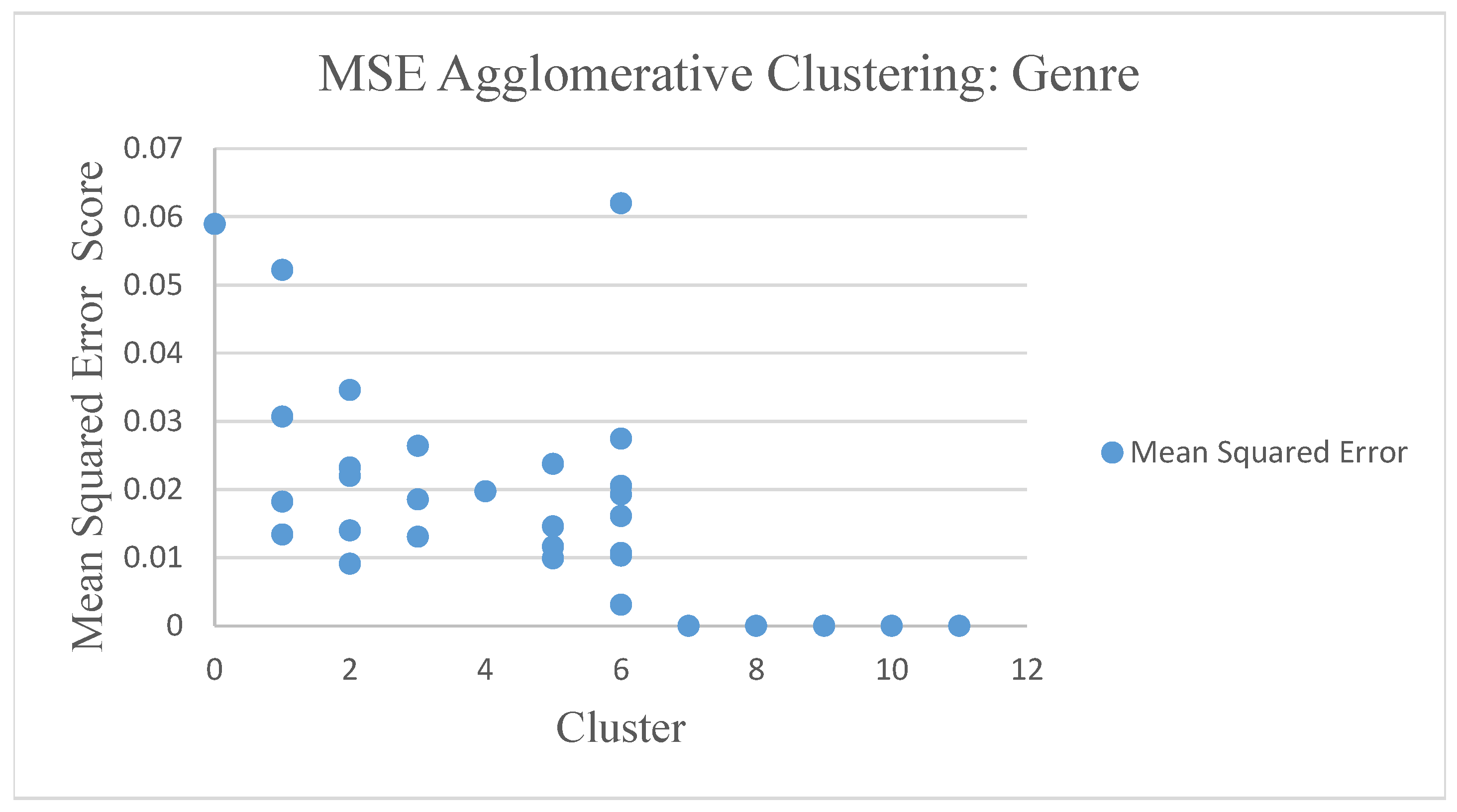
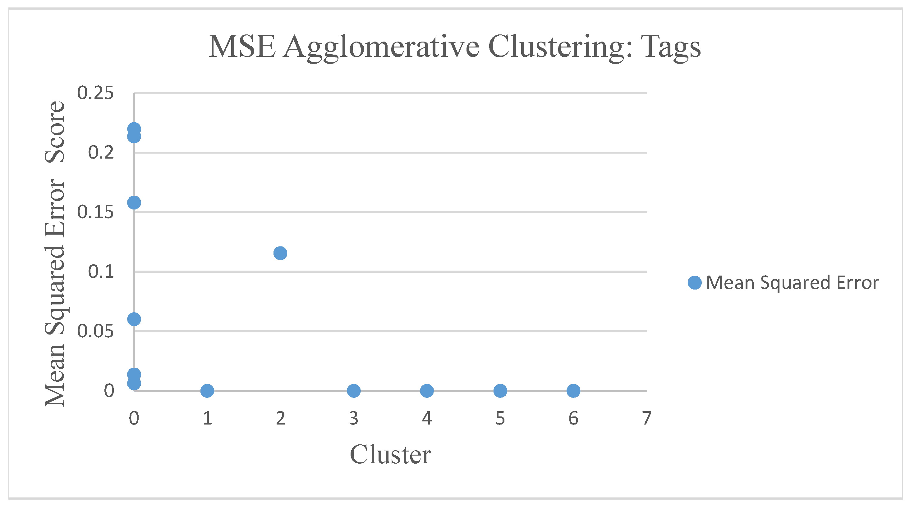
4.1.1. Mean Squared Error

Shown in Figure 12 and Figure 13, the mean squared error (MSE) agglomerative method serves as an example among the seven clustering algorithms.

4.1.2. Cluster Validity Indices: Dunn Matrix

The Dunn matrix is used as a validity measure to compare performance methods of recommendation systems. The following Dunn matrix results are shown in

Table 1. Dunn Matrix of seven clustering algorithms.

Methods	Amount of Clusters	Score
K-Means algorithm: genre rating	3	0.41
K-Means algorithm: tags rating	3	0.41
birch algorithm: genre rating	3	0.49
birch algorithm: tags rating	3	0.63
mini-batch K-Means algorithm: genre rating	3	0.38
mini-batch K-Means algorithm: tags rating	3	0.37
mean-shift algorithm: genre rating	–	0.39
mean-shift algorithm: tags rating	–	0.63
affinity propagation algorithm: genre rating	–	1.06
affinity propagation algorithm: tags rating	–	0.47
agglomerative clustering algorithm: genre rating	3	0.43
agglomerative clustering algorithm: tags rating	3	0.45
spectral clustering algorithm: genre rating	–	2.09
spectral clustering algorithm: tags rating	–	4.60

.

4.1.3. Average Similarity

The average similarity birch method example results from seven clustering algorithms are shown in

Table 2. Average similarity of birch method.

Methods	Amount of Clusters	Average Similarity
birch algorithm: genre rating	3	0.99
	6	0.97
	12	0.96
birch algorithm: tags rating	4	0.97
	6	0.93
	12	0.94

.

4.1.4. Social Network Analysis

Mean-shift results from seven clustering methods for social network analysis (SNA) are shown in

Table 3. Mean-shift social network analysis result.

Methods	Cluster	SNA
mean-shift algorithm: genre rating	Cluster: (0, 2, 1, 4)	Degree, density in cluster 0 (the highest number in result), compare to sequence list of the cluster where the distance result is 5831.49.
		Closeness, the highest in cluster 0 to cluster 1 (both clusters have a high linkage relationship) where the distance result is 1.44.
		Betweenness, the highest in cluster 0 (first) to cluster 2 (end), between 1 (cluster 0 is the most have a relationship where the cluster 1(between) and 2 where the distance result is 1.39.
mean-shift algorithm: tags rating	Cluster: (3, 0, 1, 2)	Degree, the density in cluster 0 (the highest number in result), compare to sequence list of the cluster where the distance result is 148.11.
		Closeness, the highest in cluster 0 to cluster 1 (both clusters have a high linkage relationship) where the distance result is 0.67.
		Betweenness, the highest in cluster 3 (first) to cluster 1 (end), between 0 (cluster 3 is the most have a relationship with cluster 0 (between) and 1 where the distance result is 3.12.

.

4.1.5. Association Rule: Apriori Algorithm

The association rule with Apriori algorithm is used as an evaluation measure to compare the method performance of the recommendation systems. An example of results for association rules with the Apriori algorithm from seven clustering algorithms is shown in the following section.

Rule: 12 Angry men (1957) -> Adventures of Priscilla, Queen of the Desert, The (1994) Support: 0.25 Confidence: 1.0 Lift: 4.0 ======================================== Rule: 12 Angry Men (1957) -> Airplane! (1980) Support: 0.25 Confidence 1.0 Lift: 4.0 ======================================== Rule: Amadeus (1984) -> 12 Angry men (1957) Support: 0.25 Confidence: 1.0 Lift: 4.0 ======================================== Rule: American Beauty (1999) -> 12 Angry Men (1957) Support: 0.25 Confidence: 1.0 Lift: 4.0 ======================================== Rule: Austin Powers: International Man of Mystery (1997) -> 12 Angry Men (1957) Support: 0.25 Confidence: 1.0 Lift: 4.0

4.1.6. Computational Time

The computational time is used as an evaluation measure to compare performance methods of recommendation systems. Computational time results are reported below (see

Table 4. Computational time of seven clustering algorithms.

Clustering Method	Computational Time [ms]
K-Means-genre	31.16
K-Means-tags	14.43
birch-genre	24.49
birch-tags	15.34
mini-batch K-Means method-genre	23.82
mini-batch K-Means method-tags	15.79
mean-shift-genre	13.75
mean-shift-tags	10.15
affinity propagation-genre	20.04
affinity propagation-tags	8.53
agglomerative clustering-genre	32.00
agglomerative clustering-tags	10.37
spectral clustering-genre	15.55
spectral clustering-tags	6.22

).

4.1.7. Clustering Performance Evaluation

Clustering performance evaluation (CPE) result of K-Means and birch method examples from seven clustering algorithms are reported below (see

Table 5. Clustering performance evaluation of K-Means method and birch method.

Methods	Clustering Performance Evaluation	Score
K-Means algorithm: genre rating	Silhouette Coefficient	0.29
	Calinski Harabaz Index	59.41
	Davies Bouldin Index	1.13
K-Means algorithm: tags rating	Silhouette Coefficient	0.25
	Calinski Harabaz Index	7.47
	Davies Bouldin Index	0.86
birch algorithm: genre rating	Silhouette Coefficient	0.23
	Calinski Harabaz Index	39.03
	Davies Bouldin Index	1.24
birch algorithm tags rating	Silhouette Coefficient	0.25
	Calinski Harabaz Index	5.73
	Davies Bouldin Index	1.16

).

4.2. Discussion

A detailed explanation of the above-mentioned experiments is discussed in the subsequent section. In general, for all of these methods, the higher the value of the lift, support, and confidence, the better the link is for the recommender system. Further, the higher the Dunn index value, the better the grouping.

4.2.1. K-Means Performance

Movie recommender quality is evaluated with K-Means. MSE results from K-Means show different results for genre rating and rating tags. The rating tag results are relatively smaller with rating genre scores of 0–0.95 and rating tags scores of 0–0.28. K-Means has a Dunn Matrix that tends to be evenly distributed for genre and tags with values of 0.41. The higher the Dunn index value, the better the grouping. The average similarity in the genre showed that the value increases as the number of clusters decreases. The average similarity in K-Means tags shows that the high similarity value depends on the number of clusters. The association rule with Apriori algorithm in K-Means clustering approach 13% support for the genre and 25% for tags of customers who choose movies A and B. Support is an indication of how often the itemset appears in linkages. The confidence is 61% for the genre and 100% for tags of the customers who choose movie A and movie B. Lift represents the ratio of 3.3 for genre and 4.0 for tags of the observed support value. This is a conditional probability. Clustering performance evaluation showed that the K-Means method showed good performance with the Calinski-Harabaz Index with a score of 59.41.

4.2.2. Birch Performance

To evaluate the movie recommender quality with birch, mean squared error (MSE) results from birch showed relatively small results with a rating genre score range of 0–0.25 and tag scores of 0–0.17. Birch tag ratings have a Dunn Matrix value that tends to be greater than 0.64. The average similarity in the birch genre showed that the value increases, as the number of clusters decreases. The average similarity in birch tags revealed that the high similarity value depended on the number of clusters. The association rule with Apriori algorithm in the birch clustering approach provides 16% support for genre and 50% support for tags of customers who choose movies A and B. Support is an indication of how often the itemset appears in linkages. Confidence is 100% for the genre and 50% for tags of the customers who choose movie A and B. Lift represents the ratio of 4.0 for genre and 1.0 for tags of the observed support value. The performance evaluation showed that this method provides good performance with a score of 1.24 on the Davies–Bouldin Index.

4.2.3. Mini-Batch K-Means Performance

To evaluate movie recommender quality with mini-batch K-Means, MSE results from mini-batch K-Means showed different results in genre rating and rating tags. The rating tag results were relatively smaller with a rating genre score range of 0–0.69 and rating tag scores of 0–0.19. The mini-batch K-Means with genre rating has a Dunn Matrix value that tends to be greater than 0.38. The average similarity in the mini-batch K-Means genre showed that the high similarity value depended on the number of clusters. The average similarity in the mini-batch K-Means tags showed that the high similarity value depended on the number of clusters. The association rule with Apriori algorithm in mini-batch K-Means clustering approach provides 13% support for genre and 14% support for tags of customers who choose movies A and B. Support is an indication of how often the itemset appears in linkages. Confidence is 100% for the genre and 100% for tags of the customers who choose movie A and movie B. Lift represents the ratio of 3.75 for genre and 7.0 for tags of the observed support value. The evaluation showed that the mini-batch K-Means method performs well with Calinski-Harabaz Index with a score of 48.18.

4.2.4. Mean-Shift Performance

To evaluate the movie recommender quality with the mean-shift, the MSE results from the mean-shift showed relatively larger results with a genre rating score range of 0–1 and a tag score of 0–1. The mean-shift algorithm with rating tags has a Dunn Matrix value that tends to be greater than 0.63. The average similarity in the mean-shift genre showed that the value increases as the number of clusters decreases. The average similarity in tags mean-shift showed that the high similarity value depended on the number of clusters. The mean-shift in the genre has the best computational time at 13.75 ms. The association rule with Apriori algorithm in mean-shift clustering approach provides 12% support for genre and 9% for tags of customers who choose movies A and B. Support is an indication of how often the itemset appears in linkages. Confidence is 81% for the genre and 100% for tags of the customers who choose movie A and movie B. Lift represents a ratio of 3.06 for genre and 5.5 for tags of the observed support value. The above-mentioned evaluation depicts the affinity propagation method to provide sufficient performance with Calinski-Harabaz Index with a score of 20.14.

4.2.5. Affinity Propagation Performance

To evaluate the quality with affinity propagation movie, the results of the mean squared error (MSE) from affinity propagation showed different results for genre rating and rating tags. The rating genre results were relatively smaller with a genre rating score range of 0–0.17 and a rating tag score of 0–0.89. The affinity propagation algorithm with genre rating has a Dunn Matrix which tends to be higher at 1.06. The average similarity in the affinity propagation genre showed that the high similarity value depended on the number of clusters. The average similarity in affinity propagation tags showed that the high similarity value depended on the number of clusters. The association rule with Apriori algorithm in affinity propagation clustering approach provided 10.5% support for the genre and 20% support for tags of customers who choose movies A and B. Support is an indication of how often the itemset appears in linkages. Here, 66% confidence is noted for the genre and 100% for tags of the customers who choose movie A and movie B. Lift represents the ratio of 4.22 for genre and 5.0 for tags of the observed support value. Clustering performance evaluation also showed that the affinity propagation method showed good performance with the Calinski-Harabaz Index with a score of 53.49.

4.2.6. Agglomerative Clustering Performance

Now we evaluate the movie recommender quality with agglomerative clustering. MSE results from agglomerative clustering showed different results in genre rating and rating tags. The rating genre results were relatively smaller with rating genres scores of 0–0.06 and rating tags scores with 0–0.23. Agglomerative clustering algorithms with rating tags have Dunn Matrix results that tend to be greater than 0.45. The average similarity in the agglomerative clustering genre showed that the high similarity value depended on the number of clusters. The average similarity in agglomerative clustering tags showed that the high similarity value depended on the number of clusters. The association rule with the Apriori algorithm in agglomerative clustering approach provides 22% support for the genre and 16% for tags of customers who choose movies A and B. Support is an indication of how often the itemset appears in linkages. In addition, 22% confidence is noted for the genre and 16% for tags of customers who choose movie A and movie B. Lift represents a ratio of 1.0 for genre and 1.0 for tags of the observed support value. From the performance evaluation, we see that the agglomerative clustering method performs well with the Calinski-Harabaz Index with a score of 49.34.

4.2.7. Spectral Clustering Performance

Now we evaluate the movie recommender quality with spectral clustering. Mean squared error (MSE) results from spectral clustering showed differences in genre rating and rating tags. The rating tag results were relatively smaller with a rating genre score range of 0–0.62 and rating tags scores of 0–0.17. Spectral clustering algorithm with tag rating has the best Dunn Matrix results at 4.61 and the best spectral clustering algorithm results with genre at 2.09. The average similarity in the spectral clustering genre showed that the high similarity value depended on the number of clusters. The average similarity in spectral clustering tags showed that the high similarity value depended on the number of clusters. Spectral clustering in tags has the best computational time at 6.22 ms. The association rule with Apriori algorithm in spectral clustering approach provides 12% support for the genre and 33% support for tags of customers who choose movies A and B. Support is an indication of how often the itemset appears in linkages. Confidence is 75% for the genre and 100% for tags of the customers who choose movie A and movie B. Lift represents the ratio of 3.12 for genre and 3.0 for tags of the observed support values. Clustering performance evaluation showed that the spectral clustering method showed good performance with the Calinski-Harabaz Index with a score of 16.39.

5. Conclusions

In this study, seven clusterings were used to cluster performance comparison methods for movie recommendation systems, such as the K-Means algorithm, birch algorithm, mini-batch K-Means algorithm, mean-shift algorithm, affinity propagation algorithm, agglomerative clustering algorithm, and spectral clustering algorithm. The developed optimized groupings from several algorithms were then used to compare the best algorithms with regard to the similarity groupings of users on movie genre, tags, and rating using the MovieLens dataset. Then, optimizing K for each cluster did not significantly increase the variance. To better understand this method, variance refers to the error. One of the ways to calculate this error is to extract the centroid of its respective groups. Then, this value is squared (to remove the negative terms) and all those values are added to obtain the total error. To verify the quality of the recommender system, the mean squared error (MSE), Dunn Matrix as cluster validity indices and social network analysis (SNA) were used. In addition, average similarity, computational time, association rule with Apriori algorithm and clustering performance evaluation measures were used to compare the methods of performance systems.

Using the MovieLens dataset, experiment evaluation of the seven clustering methods revealed the following:

• The best mean squared error (MSE) value is produced by the birch method with a relatively small squared error score in the rating genre and rating tags.
• Spectral clustering algorithm with tag rating has the best Dunn Matrix results at 4.61 and the spectral clustering algorithm has the best genre results at 2.09. The higher the Dunn index value is, the better the grouping.
• The closest distance to the social network analysis (SNA) is the mean-shift method, which indicates that the distance between clusters has a high linkage relationship invariance.
• The birch method had a relatively high average similarly to increase the number of clusters, which showed a good level of similarity in clustering.
• The best computational time is indicated by the mean-shift for genre at 13.75 ms and spectral clustering for tags at 6.22 ms.
• Visualization of clustering and optimizing k for movie genre in algorithms is better than movie tags because fewer data are used for movie tags.
• Mini-batch K-Means clustering approach is the best approach for the association rule with Apriori algorithm with a high score of support, 100% confidence, and 7.0 ratio of lift for item recommendations.
• Clustering performance evaluation shows that the K-Means method exhibits good performance with the Calinski-Harabaz Index with a score of 59.41, and the birch algorithm with a score of 1.24, on the Davies–Bouldin Index.
• Birch is the best method based on a comparison of several performance matrices.

References

1. Isinkaye, F.; Folajimi, Y.; Ojokoh, B. Recommendation systems: Principles, methods and evaluation. Egypt. Inform. J. 2015, 16, 261–273. [Google Scholar] [CrossRef] [Green Version]
2. Nilashi, M.; Salahshour, M.; Ibrahim, O.; Mardani, A.; Esfahani, M.D.; Zakuan, N. A new method for collaborative filtering recommender systems: The case of yahoo! movies and tripadvisor datasets. J. Soft Comput. Decis. Support Syst. 2016, 3, 44–46. [Google Scholar]
3. Smith, B.; Linden, G. Two decades of recommender systems at Amazon. com. IEEE Int. Comput. 2017, 21, 12–18. [Google Scholar] [CrossRef]
4. Greenstein-Messica, A.; Rokach, L. Personal price aware multi-seller recommender system: Evidence from eBay. Knowl. Syst. 2018, 150, 14–26. [Google Scholar] [CrossRef]
5. Itmazi, J.; Megías, M. Using recommendation systems in course management systems to recommend learning objects. Int. Arab J. Inform. Technol. 2008, 5, 234–240. [Google Scholar]
6. Kumar, M.; Yadav, D.; Singh, A.; Gupta, V.K. A movie recommender system: Movrec. Int. J. Comput. Appl. 2015, 124, 7–11. [Google Scholar] [CrossRef]
7. Lu, J.; Wu, D.; Mao, M.; Wang, W.; Zhang, G. Recommender system application developments: A survey. Decis. Support Syst. 2015, 74, 12–32. [Google Scholar] [CrossRef]
8. Shah, N.; Mahajan, S. Document clustering: A detailed review. Int. J. Appl. Inform. Syst. 2012, 4, 30–38. [Google Scholar] [CrossRef]
9. Yang, M.S.; Sinaga, K.P. A Feature-Reduction Multi-View k-Means Clustering Algorithm. IEEE Access 2019, 7, 114472–114486. [Google Scholar] [CrossRef]
10. Wu, J.L.; Chang, P.C.; Tsao, C.C.; Fan, C.Y. A patent quality analysis and classification system using self-organizing maps with support vector machine. Appl. Soft Comput. 2016, 41, 305–316. [Google Scholar] [CrossRef]
11. Qu, X.; Yang, L.; Guo, K.; Ma, L.; Feng, T.; Ren, S.; Sun, M. Statistics-Enhanced Direct Batch Growth Self-Organizing Mapping for Efficient DoS Attack Detection. IEEE Access 2019, 7, 78434–78441. [Google Scholar] [CrossRef]
12. Lv, Z.; Liu, T.; Shi, C.; Benediktsson, J.A.; Du, H. Novel land cover change detection method based on K-means clustering and adaptive majority voting using bitemporal remote sensing images. IEEE Access 2019, 7, 34425–34437. [Google Scholar] [CrossRef]
13. Wang, Z.; Yu, X.; Feng, N.; Wang, Z. An improved collaborative movie recommendation system using computational intelligence. J. Vis. Lang. Comput. 2014, 25, 667–675. [Google Scholar] [CrossRef]
14. Himel, M.T.; Uddin, M.N.; Hossain, M.A.; Jang, Y.M. Weight based movie recommendation system using K-means algorithm. In Proceedings of the 2017 International Conference on Information and Communication Technology Convergence (ICTC), Jeju-do, Korea, 18–20 October 2017; pp. 1302–1306. [Google Scholar]
15. Hajjar, M.; Aldabbagh, G.; Dimitriou, N.; Win, M.Z. Hybrid clustering scheme for relaying in multi-cell LTE high user density networks. IEEE Access 2017, 5, 4431–4438. [Google Scholar] [CrossRef]
16. Dhanachandra, N.; Manglem, K.; Chanu, Y.J. Image segmentation using K-means clustering algorithm and subtractive clustering algorithm. Procedia Comput. Sci. 2015, 54, 764–771. [Google Scholar] [CrossRef] [Green Version]
17. Arora, P.; Varshney, S. Analysis of k-means and k-medoids algorithm for big data. Procedia Comput. Sci. 2016, 78, 507–512. [Google Scholar] [CrossRef] [Green Version]
18. Yang, Y.; Wu, L.; Guo, J.; Liu, S. Research on distributed Hilbert R tree spatial index based on BIRCH clustering. In Proceedings of the 2012 20th International Conference on Geoinformatics, Hong Kong, China, 15–17 June 2012; pp. 1–5. [Google Scholar]
19. Peng, K.; Leung, V.C.; Huang, Q. Clustering approach based on mini batch kmeans for intrusion detection system over big data. IEEE Access 2018, 6, 11897–11906. [Google Scholar] [CrossRef]
20. Chen, Y.; Hu, P.; Wang, W. Improved K-Means Algorithm and its Implementation Based on Mean Shift. In Proceedings of the 2018 11th International Congress on Image and Signal Processing, BioMedical Engineering and Informatics (CISP-BMEI), Beijing, China, 13–15 October 2018; pp. 1–5. [Google Scholar]
21. Sohn, I.; Lee, J.H.; Lee, S.H. Low-energy adaptive clustering hierarchy using affinity propagation for wireless sensor networks. IEEE Commun. Lett. 2016, 20, 558–561. [Google Scholar] [CrossRef]
22. Zhang, X.; Xu, Z. Hesitant fuzzy agglomerative hierarchical clustering algorithms. Int. J. Syst. Sci. 2015, 46, 562–576. [Google Scholar] [CrossRef]
23. Shang, R.; Zhang, Z.; Jiao, L.; Wang, W.; Yang, S. Global discriminative-based nonnegative spectral clustering. Pattern Recognit. 2016, 55, 172–182. [Google Scholar] [CrossRef]
24. Harper, F.M.; Konstan, J.A. The movielens datasets: History and context. Acm Trans. Interact. Intell. Syst. 2016, 5, 19. [Google Scholar] [CrossRef]
25. Robert, C. Cluster Analysis: Correlation Profile and Orthometric (Factor) Analysis for the Isolation of Unities in Mind and Personality; Edwards Brothers: Ann Arbor, MI, USA, 1939. [Google Scholar]
26. Cox, R.W.; Chen, G.; Glen, D.R.; Reynolds, R.C.; Taylor, P.A. FMRI clustering in AFNI: False-positive rates redux. Brain Connect. 2017, 7, 152–171. [Google Scholar] [CrossRef] [PubMed]
27. Wagstaff, K.; Cardie, C.; Rogers, S.; Schrödl, S. Constrained k-means clustering with background knowledge. ICML 2001, 1, 577–584. [Google Scholar]
28. Kodinariya, T.M.; Makwana, P.R. Review on determining number of Cluster in K-Means Clustering. Int. J. 2013, 1, 90–95. [Google Scholar]
29. Liang, N.; Zheng, H.T.; Chen, J.Y.; Sangaiah, A.; Zhao, C.Z. TRSDL: Tag-Aware Recommender System Based on Deep Learning–Intelligent Computing Systems. Appl. Sci. 2018, 8, 799. [Google Scholar] [CrossRef] [Green Version]
30. Massart, D.L.; Kaufman, L.; Rousseeuw, P.J.; Leroy, A. Least median of squares: A robust method for outlier and model error detection in regression and calibration. Anal. Chim. Acta 1986, 187, 171–179. [Google Scholar] [CrossRef]
31. Sheikholeslami, G.; Chatterjee, S.; Zhang, A. Wavecluster: A multi-resolution clustering approach for very large spatial databases. VLDB 1998, 98, 428–439. [Google Scholar]
32. Maimon, O.; Rokach, L. Data Mining and Knowledge Discovery Handbook; Springer: Berlin/Heidelberg, Germany, 2005. [Google Scholar]
33. Fukunaga, K.; Hostetler, L. The estimation of the gradient of a density function, with applications in pattern recognition. IEEE Trans. Inform. Theory 1975, 21, 32–40. [Google Scholar] [CrossRef] [Green Version]
34. Dueck, D. Affinity Propagation: Clustering Data by Passing Messages; University of Toronto: Toronto, ON, Canada, 2009. [Google Scholar]
35. Rukmi, A.M.; Iqbal, I.M. Using k-means++ algorithm for researchers clustering. In AIP Conference Proceedings; AIP Publishing: Melville, NY, USA, 2017; Volume 1867, p. 020052. [Google Scholar]
36. Freeman, L. The Development of Social Network Analysis; A Study in the Sociology of Science; Empirical Press: New York, NY, USA, 2004; Volume 1. [Google Scholar]
37. Plattel, C. Distributed and Incremental Clustering Using Shared Nearest Neighbours. Master’s Thesis, Utrecht University, Utrecht, The Netherlands, 2014. [Google Scholar]
38. Malik, J.S.; Goyal, P.; Sharma, A.K. A Comprehensive Approach towards Data Preprocessing Techniques & Association Rules. In Proceedings of the 4th National Conference. 2010. Available online: http://bvicam.ac.in/news/INDIACom%202010%20Proceedings/papers/Group3/INDIACom10_279_Paper%20(2).pdf (accessed on 24 December 2019).
39. Maulik, U.; Bandyopadhyay, S. Performance evaluation of some clustering algorithms and validity indices. IEEE Trans. Pattern Anal. Mach. Intell. 2002, 24, 1650–1654. [Google Scholar] [CrossRef] [Green Version]
Figure 1. Similarities within people to build a movie recommendation system for users.
Symmetry 12 00185 g001
Figure 2. Flowchart that configures a recommendation system for movies.
Symmetry 12 00185 g002
Figure 3. Visualization of K-Means clustering algorithms. K-Means genre (a), K-Means tag (b).
Symmetry 12 00185 g003
Figure 4. Visualization of birch clustering algorithms. Birch genre (a), birch tag (b).
Symmetry 12 00185 g004
Figure 5. Visualization of mini-batch K-Means clustering. Mini-batch K-Means genre (a), mini-batch K-Means tag (b).
Symmetry 12 00185 g005
Figure 6. Visualization of mean-shift clustering algorithms. Mean-shift genre (a), mean-shift tag (b).
Symmetry 12 00185 g006
Figure 7. Visualization of affinity propagation clustering algorithms. Affinity propagation genre (a), affinity propagation tag (b).
Symmetry 12 00185 g007
Figure 8. Visualization of agglomerative clustering algorithm. Agglomerative clustering genre (a), agglomerative clustering tag (b).
Symmetry 12 00185 g008
Figure 9. Visualization of spectral clustering algorithm. Spectral clustering genre (a), spectral clustering tag (b).
Symmetry 12 00185 g009
Figure 10. Example for visualization Genre K-Means of Top list-N of movies.
Symmetry 12 00185 g010
Figure 11. Example of visualization optimization of K in K-Means genre rating.
Symmetry 12 00185 g011
Figure 12. MSE agglomerative clustering genre.
Symmetry 12 00185 g012
Figure 13. MSE agglomerative clustering tags.
Symmetry 12 00185 g013