Adaptive Stabilization of a Fractional-Order System with Unknown Disturbance and Nonlinear Input via a Backstepping Control Technique

College of Intelligent Science and Control Engineering, Jinling Institute of Technology, Nanjing 211169, China
*
Authors to whom correspondence should be addressed.
Symmetry 2020, 12(1), 55; https://doi.org/10.3390/sym12010055
Submission received: 28 November 2019
/
Revised: 19 December 2019
/
Accepted: 23 December 2019
/
Published: 26 December 2019
Abstract
:In this paper, a new backstepping-based adaptive stabilization of a fractional-order system with unknown parameters is investigated. We assume that the controlled system is perturbed by external disturbance, the bound of external disturbance to be unknown in advance. Moreover, the effects of sector and dead-zone nonlinear inputs both are taken into account. A fractional-order auxiliary system is established to generate the necessary signals for compensation the nonlinear inputs. Meantime, in order to deal with these unknown parameters, some fractional-order adaption laws are given. The frequency-distributed model is used so that the indirect Lyapunov theory is available in designing controllers. Finally, simulation results are presented to verify the effectiveness and robustness of the proposed control strategy.
1. Introduction
Fractional-order calculus derives from the end of 17th century; it is particularly suitable for describing the viscoelastic system [1], and the memory and hereditary properties of various materials and processes. Symmetries play an important role in dynamics of fractional-order systems, and some results have been reported about the fractional symmetry; for instance, Frederico and Torres [2] studied fractional Noether symmetry and gave a definition of a fractional conserved quantity. Zhang [3,4] investigated Noether symmetry and conserved quantity for the classical fractional Birkhoffian system and the fractional Birkhoffian system with time delay. Song [5] researched Noether quasi-symmetry and perturbation to Noether quasi-symmetry. Now, studying fractional-order systems has became an active research area. In particular, control and stabilization of the fractional-order systems have attracted much attention from various scientific fields. It has been proven that applying fractional-order controllers to fractional-order system can obtain a better control effect than integer-order controllers, such as fractional-order PID control [6], fractional-order sliding mode control [7], fractional fuzzy control [8], fractional-order finite-time control [9], and so on.
The backstepping method is a recursive approach for controller design; through designing virtual controllers and partial Lyapunov functions step by step, a common Lyapunov function of the whole system can be deduced from the above operations. This method can guarantee the global stability, tracking, and transient performance of nonlinear systems [10]. In view of the excellent performance of backstepping, an increasing number of researchers have focused on this potential problem. Many studies for the backstepping-based control and synchronization of fractional-order chaotic system have been reported. For example, Luo [11] researched the robust control and synchronization of a fractional-order system by adding one power integrator. Shukla [12,13] realized the stabilization and synchronization of fractional-order chaotic systems by using backstepping method. Wei [14,15] investigated the stability of fractional-order nonlinear systems via the adaptive backstepping technique.
However, all approaches in the aforementioned works are only focused on the linear and direct application of control inputs. In practice, input nonlinearity is often encountered in various systems and can be a cause of instability. Thus, it is obvious that the effects of input nonlinearity must be taken into account when analyzing and implementing a control scheme. Recently, Sheng [16] and Ha [17] considered the impacts of input saturation in the stabilization or synchronization of fractional-order systems. To the best of our knowledge, there is little information available in the literature about the stabilization of fractional-order systems with more complicated nonlinear inputs. Meanwhile, applying the backstepping approaches to a fractional-order system with unknown bounded external disturbances is also rare.
Motivated by the above discussions, it is still very challenging and essential to research the stabilization of fractional-order systems with complex nonlinear input by using adaptive backstepping techniques. Sector and dead-zone nonlinear inputs are more complicated than saturated input in characteristics, thus, in this paper, on the basis of symmetry principles, the effects of sector and dead-zone nonlinear inputs both are considered. For compensation of the nonlinear inputs, a fractional-order auxiliary system is constructed to generate necessary signals. For efficient handling of a system with unknown parameters, some new adaptive estimation rules are proposed. The frequency-distributed model is used to establish an indirect Lyapunov function to demonstrate the stability and design a virtual controller for every subsystem. Through the design of a virtual controller, a comprehensive actual controller and unknown disturbance estimation rule are determined.
To sum up, our approach makes the following contributions: (i) The backstepping-based stabilization of fractional-order systems with unknown bounded external disturbance is researched; (ii) The effects of two kinds of nonlinear inputs with complicated characteristic are considered; (iii) A fractional order auxiliary system is constructed to generate virtual signals for compensation of the sector and dead-zone nonlinear inputs; (iv) Based on the frequency-distributed model, indirect Lyapunov theory is used to design controllers and some adaptive estimation laws are established.
The remaining part of this paper is organized as follows: Section 2 introduces the relevant definitions, frequency-distributed model and strict feedback system. Main results are presented in Section 3. Some numerical simulations are provided in Section 4 to show the effectiveness of the proposed method. Finally, conclusions are given in Section 5.
2. Preliminaries and System Description
Definition 1
(see [18]). The Caputo’s fractional derivative of order α of function is
where m is the smallest integer number, larger than α. In the rest of this paper, we will use instead of .
Lemma 1
Strict feedback system [22] can be used to express different real world systems, which can be described as follows
where is the system parameters vector of the i-th state equation, , , for are known, smooth nonlinear functions. When consider the effects of external disturbance and the sector and dead-zone nonlinear inputs , meantime, the system parameters vector is unknown, , , …, are constants, then the system can be rewritten as
where is the comprehensive actual controller to be designed later. is a nonlinear input function, if it is continuous inside a sector and satisfying the following equation
in (5), , then is called sector nonlinear input. A typical and symmetrical sector nonlinear function is shown in Figure 1.
The dead-zone nonlinear function is described as follows
where and are nonlinear functions of , and are given constants. Besides, outside of the dead-band, the nonlinear input has gain reduction tolerances , , and , which satisfy the following symmetric property
in which, , , and are positive constants. A sample dead-zone nonlinear function is displayed in Figure 2.
Before introducing our approach, we firstly give an assumption.
Assumption 1.
Suppose there exist an unknown constantsuch that the external disturbance satisfies.
Next, the main control strategy will be introduced in detail, the frequency distributed model is used so that the indirect Lyapunov theory can be applied to demonstrate the feasibility of the proposed control scheme [23,24,25,26,27,28]. In simulation, the numerical method [29] is used to solve the fractional order equations, two examples about fractional-order Chua system and fractional-order Rossler’s [30] system are given to verify the correctness of the presented control method.
3. Main Results
This section introduces the adaptive backstepping-based stabilization of fractional-order system with nonlinear input and external disturbance, to deduce the actual controller, transformation variables should be assigned firstly as
where for is the virtual signal generated by the following auxiliary fractional-order system to compensate the sector and dead-zone nonlinear inputs
in which, , , , . is virtual controller and can be designed as
where . is the abbreviation of . is the estimation of unknown parameters vector . is the estimation of . Denote and as the estimation errors, the parameters update laws are chosen as
Theorem 1.
Consider the system (4) with sector nonlinear input, the controller which leads to asymptotic stabilization of system is given below
Proof.
Step 1: The first new subsystem can be obtain according to Equations (4) and (8)
according to Lemma 1, the new subsystem (13) and parameters adaptation laws (11) can be transformed into the frequency distributed model, that is
in Equation (14), , and are infinite dimension distributed state variables, while , and are the weighted sum of the variables , and , respectively. Selecting the Lyapunov function as
taking the derivative of , it yields
substituting into Equation (16), and according to Assumption 1, we have
if , the adaption law reduces to , then , that is , , are all asymptotically converge to zero.
Step 2: The Second new subsystem about can be construct as
the corresponding frequency distributed model is
in Equation (19), and are infinite dimension distributed state variables, while and are the weighted sum of the variables and , respectively. In this step to ensure converge to 0 as time tends to infinity. Selecting the Lyapunov function as
thus its derivative can be described as
substituting from Equation (10) to Equation (21), and according to Assumption 1, it yields
similar to step 1, if , the adaption law reduces to , then , that is will be ensured to converge to zero asymptotically.
Step i (i = 3, …, n − 1): We continue to investigate the i-th new subsystem with transformation variable , that is
the frequency distributed model can be described as
in Equation (24), and are infinite dimension distributed state variables, while and are the weighted sum of the variables and , respectively. This step is to verify the stability of system (23) with the following Lyapunov function
taking the derivative of , one has
introducing the virtual controller from Equation (10) into Equation (26), we obtain
that is, when , then the estimation law reduce to , so, , is asymptotically converge to zero, which returns to step i-1.
Step n: In the last step, the actual controller is designed. Similar to the above steps, the last subsystem with transformation variable is determined as
the corresponding frequency distributed model is
in Equation (29), and are infinite dimension distributed state variables, while and are the weighted sum of the variables and , respectively. the overall Lyapunov function is constructed as
according to the previous inequality are induced in the step 1 to n−1, the derivative of Equation (30) is
according to Equations (5) and (12), we known that
since , , , according to above inequality, we have
multiply both sides of inequality (33) by , and according to , , we obtain
substituting Equation (34) into Equation (31), and according to the second equation of Equation (12), one has
because of , so the controlled system (4) with sector nonlinear input is asymptotically stable, thus the proof is completed. □
Theorem 2.
Consider the system (4) with dead-zone nonlinear input, the controller which leads to asymptotic stabilization of system is given below
where, , and
Proof.
Step 1 to i (i = 2, …, n−1): Similar to the Proof of Theorem 1, for the concision, here is omitted, only deduce the final step.
Step n: The overall Lyapunov function is selected as
taking the derivative of , and using the preceding derivative , according to Assumption 1, it yields
if , and surveying Equation (36), it is clear that , then according to Equations (6) and (7), we have
since , , , according to the above inequality, we have
multiply both sides of inequality (41) by , and according to , , we get
on the basis of symmetry principles, when , through similar derivation, the inequality (42) still holds. Substituting the inequality (42) into (39), we have
that is , so the adaptive stabilization of the controlled system (4) with dead-zone nonlinear input is realized, therefore the proof is completed. □
4. Simulation Results
In this section, two simulation examples are given to demonstrate the effectiveness and feasibility of the proposed control strategy.
4.1. Adaptive Stabilization of Fractional-Order Chua System with Sector Nonlinear Input
The dynamics of fractional-order Chua system can be described as
where , is the nonlinear part of system, , , , . This system is not strict feedback form, select , , , considering external disturbance , the above system is transformed to the following strict feedback form
according to the standard form (4), we known that , , , and the unknown parameter vector , . The sector nonlinear input is given by
obviously, , , because of , so, in the auxiliary system (9), we can choose , , , , that is
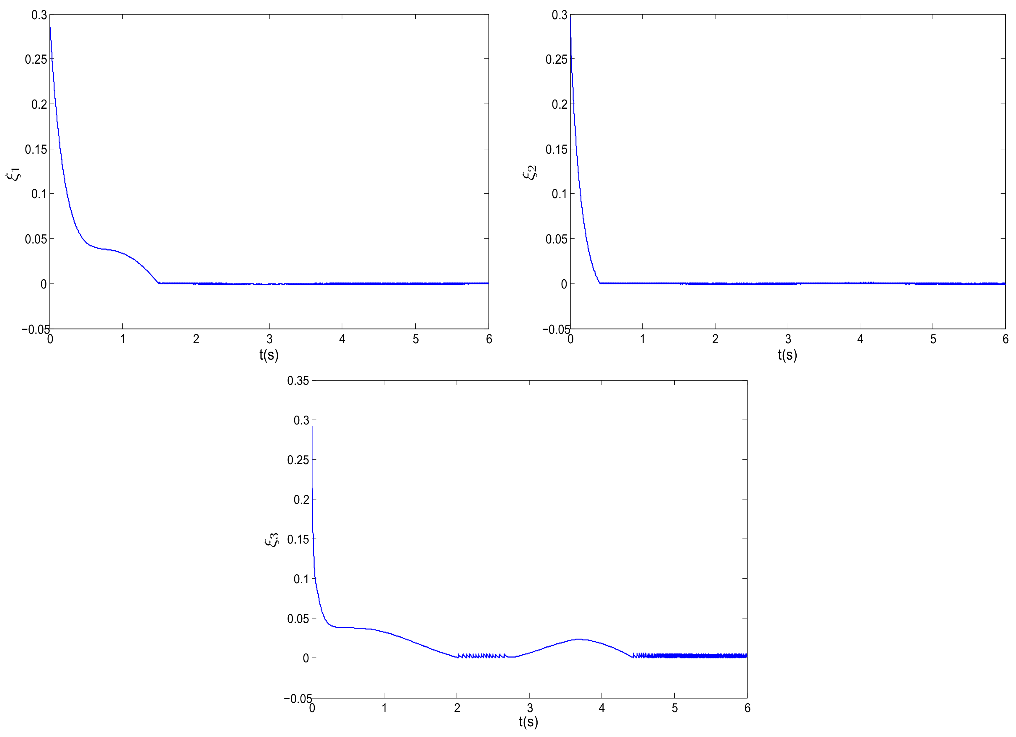
in this simulation, , , the initial values are selected as , , , , , , . When the actual controller is activated, the time response of the transformation variables are shown in Figure 3, it is obvious that all variables trajectories are asymptotically tend to zero, which implies that under the control of the proposed control strategy, the adaptive stabilization of the controlled system with sector nonlinear input is realized.
4.2. Adaptive Stabilization of Fractional-Order Rossler’s System with Dead-Zone Nonlinear Input
The fractional-order Rossler’s system can be expressed as follows
where , , , , this system can be transformed into strict feedback form by selecting , , , that is
according to the standard form (4), we known that , , , and the unknown parameter vectors , , , . is external disturbance. The dead-zone nonlinear input is given by
correspondingly, parameters , , so, , , due to , so, in the auxiliary system (9), we can choose , , , . that is
In this simulation, , , the initial values are selected as , , , , , , , . When the actual controller in (36) is activated, the time response of the transformation variables are shown in Figure 4, all variables trajectories asymptotically converge to zero. The above simulation results demonstrated the feasibility of the proposed method for fractional-order system with dead-zone nonlinear input.
Remark 1.
The theorems firstly realized the backstepping-based stabilization of the fractional-order system with sector and dead-zone nonlinear inputs, if, these methods change into the integer-order case, if α is not a fixed constant, the above theorems will be common solutions to incommensurate fractional-order systems. The indirect Lyapunov theory can ensure more degrees of freedom in designing the parameter estimation laws and can obtain better control performance.
5. Conclusions
In this paper, a backstepping-based adaptive stabilization of a fractional-order system is researched. The system is perturbed by unknown bounded external disturbance, and system parameters are unknown in advance. The effects of sector and dead-zone nonlinear inputs both are considered in design the controller. For dealing with nonlinear input, a fractional-order auxiliary system is constructed to provide virtual signals. A frequency-distributed model is adopted so that indirect Lyapunov stability theory is used to demonstrate the stability of new subsystems with transformation variables. Through design, the virtual controllers are used to deduce an overall actual controller. Simulation results demonstrated the feasibility and effectiveness of the proposed control scheme.
Author Contributions
Conceptualization, X.T.; Methodology, X.T. and Z.Y.; Software, X.T.; Validation, Z.Y.; Formal analysis, X.T.; Investigation, Z.Y.; Resources, X.T. and Z.Y.; Data curation, X.T.; Writing—original draft preparation, X.T.; Writing—review and editing, Z.Y.; Visualization, X.T. and Z.Y.; Supervision, Z.Y.; Project administration, Z.Y.; Funding acquisition, X.T. All authors have read and agreed to the published version of the manuscript.
Funding
This research received no external funding.
Acknowledgments
This work is supported by the Foundation of Jinling Institute of Technology (Grant No: jit-fhxm-201607 and jit-b-201706), the Natural Science Foundation of Jiangsu Province University (Grant No: 17KJB120003).
Conflicts of Interest
The authors declare no conflict of interest.
References
- Bagley, R.L.; Calico, R.A. Fractional order state equations for the control of viscoelastically damped structure. J. Guid. Control Dyn. 1991, 14, 304–311. [Google Scholar] [CrossRef]
- Frederico, G.S.F.; Torres, D.F.M. A formulation of Noether’s theorem for fractional problems of the calculus of variations. J. Math. Anal. Appl. 2007, 334, 834–846. [Google Scholar] [CrossRef] [Green Version]
- Zhang, Y.; Zhai, X.H. Noether symmetries and conserved quantities for fractional Birkhoffian systems. Nonlinear Dyn. 2015, 81, 469–480. [Google Scholar] [CrossRef]
- Zhai, X.H.; Zhang, Y. Noether symmetries and conserved quantities for fractional Birkhoffian systems with time delay. Commun. Nonlinear Sci. 2016, 36, 81–97. [Google Scholar] [CrossRef]
- Song, C.J. Noether symmetry for fractional Hamiltonian system. Phys. Lett. A 2019, 383, 12914. [Google Scholar] [CrossRef]
- Dumlu, A.; Erenturl, K. Trajectory tracking control for a 3-DOF parallel manipulator using fractional-order PIλDμ control. IEEE Trans. Ind. Electron. 2014, 61, 3417–3426. [Google Scholar] [CrossRef]
- Ni, J.; Liu, L.; Liu, C.; Hu, X. Fractional order fixed-time nonsingular terminal sliding mode synchronization and control of fractional order chaotic systems. Nonlinear Dyn. 2017, 89, 2065–2083. [Google Scholar] [CrossRef]
- Liu, H.; Pan, Y.; Chen, Y. Adaptive fuzzy backstepping control of fractional-order nonlinear systems. IEEE Trans. Syst. Man Cybern. Syst. 2017, 47, 2209–2217. [Google Scholar] [CrossRef]
- Aghababa, M.P.; Khanmohammadi, S.; Alizadeh, G. Finite-time synchronization of two different chaotic systems with unknown parameters via sliding mode technique. Appl. Math. Model. 2011, 35, 3080–3091. [Google Scholar] [CrossRef]
- Bigdeli, N.; Ziazi, H.A. Finite-time fractional-order adaptive intelligent backsstepping sliding mode control of uncertain fractional-order chaotic systems. J. Frankl. Inst. 2017, 354, 160–183. [Google Scholar] [CrossRef]
- Luo, R.Z.; Huang, M.C.; Su, H.P. Robust control and synchronization of 3-D uncertain fractional-order chaotic systems with external disturbances cia adding one power integrator control. Complexity 2019, 2019, 8417536. [Google Scholar] [CrossRef]
- Shukla, M.K.; Sharma, B.B. Backstepping based stabilizaiton and synchronizaiton of a class of fractional order chaotic systems. Chaos Soliton Fract. 2017, 102, 274–284. [Google Scholar] [CrossRef]
- Shukla, M.K.; Sharma, B.B. Stabilizaiton of a class of fractional order chaotic systems via backstepping approach. Chaos Soliton Fract. 2017, 98, 56–62. [Google Scholar] [CrossRef]
- Wei, Y.H.; Sheng, D.; Chen, Y.Q.; Wang, Y. Fractional order chattering-free robust adaptive backstepping control technique. Nonlinear Dyn. 2019, 95, 2383–2394. [Google Scholar] [CrossRef]
- Wei, Y.H.; Chen, Y.Q.; Liang, S.; Wang, Y. A novel algorithm on adaptive backstepping control of fractional order systems. Neurocomputing 2015, 165, 395–402. [Google Scholar] [CrossRef]
- Sheng, D.; Wei, Y.H.; Cheng, S.S.; Shuai, J.M. Adaptive backstepping control for fractional order systems with input saturation. J. Frankl. Inst. 2017, 354, 2245–2268. [Google Scholar] [CrossRef]
- Ha, S.M.; Liu, H.; Li, S.G.; Liu, A.J. Backstepping-based adaptive fuzzy synchronization control for a class of fractional-order chaotic systems with input saturation. Int. J. Fuzzy Syst. 2019, 21, 1571–1584. [Google Scholar] [CrossRef]
- Podlubny, I. Fractional Differential Equations; Academic Press: New York, NY, USA, 1999. [Google Scholar]
- Trigeassou, J.C.; Maamri, N.; Sabatier, J.; Oustaloup, A. State variables and transients of fractional order differential systems. Comput. Math. Appl. 2012, 64, 3117–3140. [Google Scholar] [CrossRef] [Green Version]
- Trigeassou, J.C.; Maamri, N.; Sabatier, J.; Oustaloup, A. Transients of fractional-order integrator and derivatives. Signal Image Video Process. 2012, 6, 359–372. [Google Scholar] [CrossRef]
- Trigeassou, J.C.; Maamri, N. Initial conditions and initialization of linear fractional differential equations. Signal Process. 2011, 91, 427–436. [Google Scholar] [CrossRef]
- Shukla, M.K.; Sharma, B.B. Control and synchronizaiton of a class of uncertain fractional order chaotic systems via adaptive backstepping control. Asian J. Control 2018, 20, 707–720. [Google Scholar] [CrossRef]
- Chen, Y.Q.; Wei, Y.H.; Zhou, X.; Wang, Y. Stability for nonlinear fractional order systems: An indirect approach. Nonlinear Dyn. 2017, 89, 1011–1018. [Google Scholar] [CrossRef]
- Wang, Y.; Liu, L.; Liu, C.X.; Zhu, Z.W.; Sun, Z.Q. Fractional-order adaptive backstepping control of a noncommensurate fractional-order ferroresonance system. Math. Probl. Eng. 2018, 8091757. [Google Scholar] [CrossRef]
- Luo, R.Z.; Wang, Y.L.; Deng, S.C. Combination synchronization of three classic chaotic systems using active backstepping design. Chaos 2011, 21, 043114. [Google Scholar]
- Liu, S.Y.; Liu, Y.C.; Wang, N. Nonlinear disturbance observer-based backstepping finite-time sliding mode tracking control of underwater vehicles with system uncertainties and external disturbances. Nonlinear Dyn. 2017, 88, 465–476. [Google Scholar] [CrossRef]
- Chen, C.P.; Wen, G.X.; Liu, Y.J.; Liu, Z. Observer-based adaptive backstepping consensus tracking control for high-order nonlinear semi-feedback multiagent systems. IEEE Trans. Cybern. 2016, 46, 1591–1601. [Google Scholar] [CrossRef]
- Ding, D.S.; Qi, D.L.; Peng, J.M.; Wang, Q. Asymptoic pseudo-state stabilization of commensurate fractional-order nonlinear systems with additive disturbance. Nonlinear Dyn. 2015, 81, 667–677. [Google Scholar] [CrossRef]
- Diethelm, K.; Ford, N. A predictor-corrector approach for the numerical solution of fractional differential equations. Nonlinear Dyn. 2002, 29, 3–22. [Google Scholar] [CrossRef]
- Li, C.; Chen, G. Chaos and hyperchaos in the fracitional-order Rossler equations. Physica A 2004, 341, 55–61. [Google Scholar] [CrossRef]
Figure 1.
Sector nonlinear function for the input .
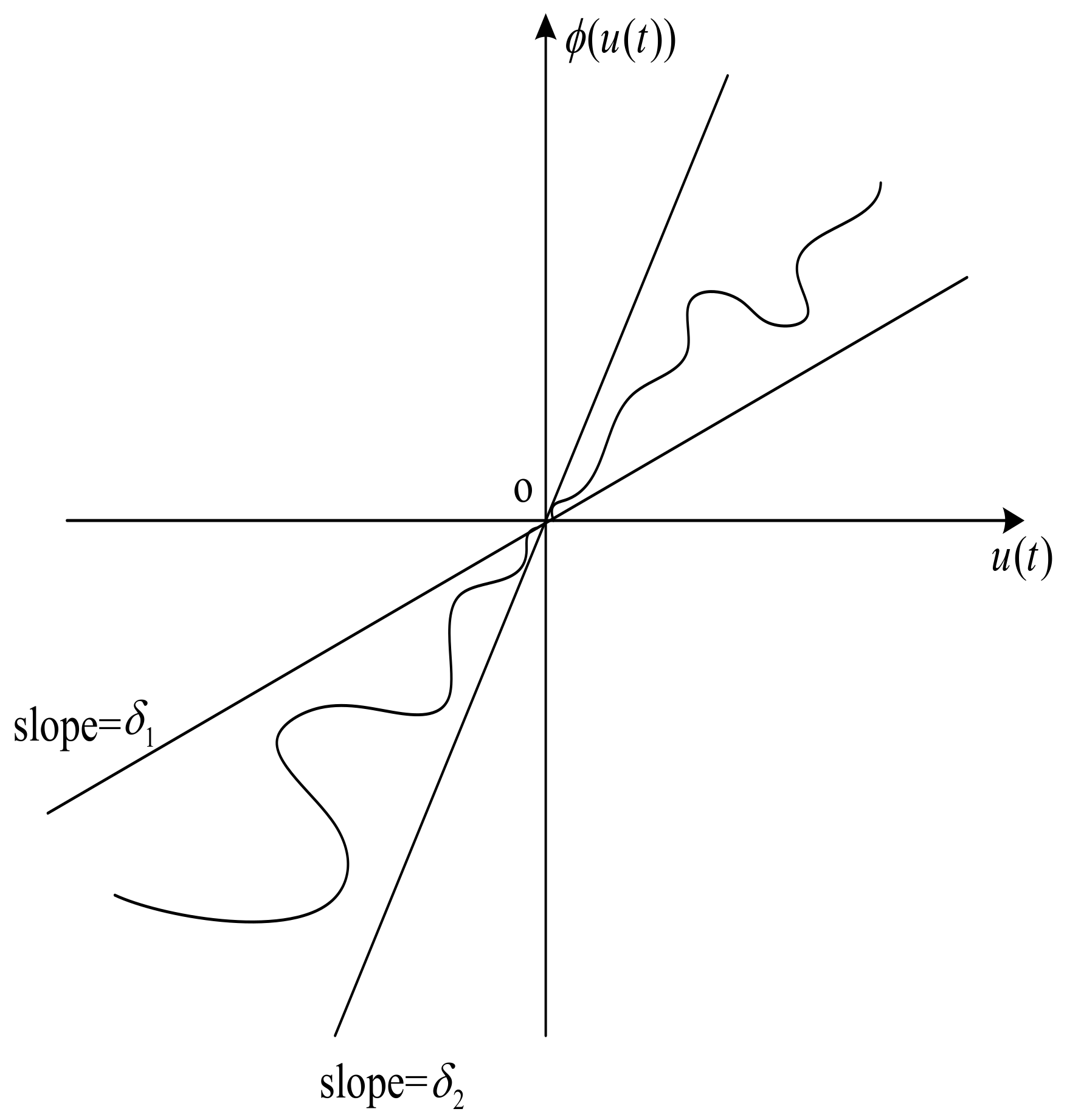
Figure 2.
Dead-zone nonlinear function for the input .
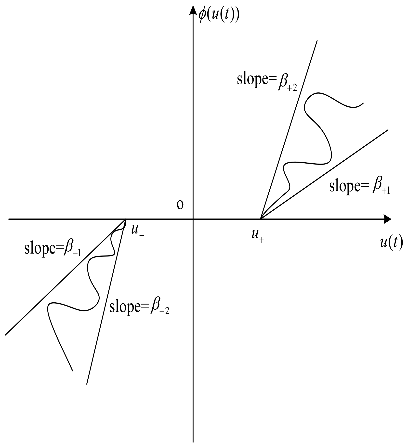
Figure 3.
Time response of the transformation variables in system (45).

Figure 4.
Time response of the transformation variables in system (49).
© 2019 by the authors. Licensee MDPI, Basel, Switzerland. This article is an open access article distributed under the terms and conditions of the Creative Commons Attribution (CC BY) license (http://creativecommons.org/licenses/by/4.0/).
Share and Cite
MDPI and ACS Style
Tian, X.; Yang, Z. Adaptive Stabilization of a Fractional-Order System with Unknown Disturbance and Nonlinear Input via a Backstepping Control Technique. Symmetry 2020, 12, 55. https://doi.org/10.3390/sym12010055
AMA Style
Tian X, Yang Z. Adaptive Stabilization of a Fractional-Order System with Unknown Disturbance and Nonlinear Input via a Backstepping Control Technique. Symmetry. 2020; 12(1):55. https://doi.org/10.3390/sym12010055
Chicago/Turabian StyleTian, Xiaomin, and Zhong Yang. 2020. "Adaptive Stabilization of a Fractional-Order System with Unknown Disturbance and Nonlinear Input via a Backstepping Control Technique" Symmetry 12, no. 1: 55. https://doi.org/10.3390/sym12010055
Note that from the first issue of 2016, this journal uses article numbers instead of page numbers. See further details here.