Abstract
In the first part of our paper, we construct a cyclic hypergroup of matrices using the Ends Lemma. Its properties are then, in the second part of the paper, used to describe the symmetry of lower and upper approximations in certain rough sets with respect to invertible subhypergroups of this cyclic hypergroup. Since our approach is widely used in autonomous robotic systems, we suggest an application of our results for the study of detection sensors, which are used especially in mobile robot mapping.
Keywords:
single-power cyclic hypergroup; invertible subhypergroup; lower approximation; upper approximation; rough set MSC:
20N20
1. Introduction
Our perception of the real world is never fully precise. Our decisions are always made with a certain level of uncertainty or lack of some pieces of information. Mathematical tools that make this decision making easier include fuzzy sets [1], rough sets [2,3] or soft sets [4]. In the algebraic hyperstructure theory, i.e., in the theory of algebraic hypercompositional structures, there are numerous constructions leading to such structures. One of these is the application of the Ends lemma [5,6,7] in which the hyperoperation is the principal end of a partially ordered semigroup. For some theoretical results regarding the construction, see for example Novák et al. [7,8,9]. In [9] the authors modify the construction in order to increase its applicability.
In our paper we develop an idea similar to [9,10,11]. With the help of matrix calculus, which we believe is a suitable tool, we construct cyclic hypergroups and their invertible subhypergroups. Notice that matrix calculus linked to the theory of algebraic hypercompositional structures has been used as a suitable tool in various contexts such as [12,13,14]. Since the notion of hypercompositional cyclicity has a rather complicated evolution, we recommend the reader to study [15], which gives a complex discussion of the topic, and [16] which is the source of our definition.
In [17] the authors consider the application of rough sets in various contexts based on establishing the set describing its upper and lower approximation. In a general case, this issue is discussed, e.g., in [11,18,19]. Suppose that we can see the Ends Lemma as a certain boundary used in various areas such as economics (the need to generate at least certain profit), electrical engineering (the transistor basis of a p-n junction needs at least certain current for the charge flow yet this must not be too great), etc. Motivated by these considerations we investigate hypercompositional structures constructed with the help of the principal end (or beginning) and their subhyperstructures. We study their cyclicity and their generators. In the context of rough sets we use cyclic hypergroups to construct the universum with the help of indiscernibility relation and its subhyperstructures describing their upper and lower approximations. In order to describe these we make use of some natural relations between matrix characteristics. In the end of our paper we demonstrate how this type of rough sets, especially the upper approximations, can be used for description of an area monitored by sensors of autonomous robotic systems.
2. Notation and Context
In our paper, we work with matrices. In a general case these are matrices over a field. However, within this field we regard a subset (infinite such as or finite such as in Example 5), elements of which are actually used as entries. We denote such a set by , and the set of all matrices with entries from a by . We also suppose that there exists a total order on with the smallest element of denoted (if it exists) by e. Within the set we, in our hyperoperations, rely on the operation , the result of which is, given our context, equal to the smaller element.
On we, for an arbitrary pair of matrices , define relation by
where , i.e., is the row norm.
Example 1.
For matrices
there is
Therefore .
Basic Notions of the Theory of Algebraic Hypercompositional Structures
Before we give our results, recall some basic notions of the algebraic hyperstructure theory (or theory of algebraic hypercompositional structures). For further reference see, for example, books [20,21]. A hypergroupoid is a pair , where H is a nonempty set and the mapping is a binary hyperoperation (or hypercomposition) on (here denotes the system of all nonempty subsets of ). If holds for all , then is called a semihypergroup. If moreover the reproduction axiom, i.e., relation for all , is satisfied, then the semihypergroup is called hypergroup. Unlike in groups, in hypergroups neutral elements or inverses need not be unique. By a neutral element, or an identity (or unit) of we mean such an element that for all while by an inverse of we mean such an element that there exists an identity such that . By idempotence in the sense of hypercompositional structures we mean that , i.e., that the element is included in its “second power” (which is, in general, a set).
Numerous notions of algebraic structures can be generalized for algebraic hypercompositional structures while some hypercompositional notions have no counterparts in algebraic structures. One of the key algebraic concepts, cyclicity, can be transferred to theory of algebraic hypercompositional structures in several ways. For a complex discussion of these approaches as well as their historical context and evolution and clarification of naming and notation, see Novák, Křehlík and Cristea [15]. In our paper we will work with the following definition introduced by Vougiouklis [16] (reworded as in [15]); for more results regarding cyclic hypergroups see Vougiouklis [22].
Definition 1
([15,16]). A hypergroup is called cyclic if, for some , there is
where and . If there exists such that Formula (2) is finite, we say that H is a cyclic hypergroup with finite period; otherwise, H is a cyclic hypergroup with infinite period. The element in Formula (2) is called generator of H, the smallest power n for which Formula (2) is valid is called period of h. If all generators of H have the same period n, then H is called cyclic with period n. If, for a given generator h, Formula (2) is valid but no such n exists (i.e., Formula (2) cannot be finite), then H is called cyclic with infinite period. If we can, for some , write
Then, the hypergroup H is called single-power cyclic with a generator h. If Formula (2) is valid and for all and, for a fixed , there is
then we say that H is a single-power cyclic hypergroup with an infinite period for h.
Apart from the notion of cyclicity we will work with the notion of –hyperstructures, i.e., hypercompositional structures constructed from ordered (or sometimes pre-ordered) semigroups by means of what is known as the “Ends Lemma”. For details and applications see, for example, [8,9,10,12,23].
3. Single-Power Cyclic Hypergroup of Matrices
In order to construct a single-power cyclic hypergroup of matrices, we first, for an arbitrary pair of matrices , define a hyperoperation by
where is such a matrix that and is the set of all matrices greater than , i.e., . Thus, using terminology of Chvalina [5], is an extensive hypergroupoid, i.e., for an arbitrary pair of matrices there is . Notice that some other authors, motivated by the geometrical meaning, call such hypergroupoids “closed” as contrasted to “open”.
Example 2.
For matrices and from Example 1 we have:
Remark 1.
With the above example we not only demonstrate the meaning of the hyperoperation “∗” but also provide an example to the forthcoming Lemma 3. In this respect notice that , and , which means that . Since in our paper we regard as a part of , writing the hyperoperation (5) explicitly in the form of union is not neccessary. However, for, as an example, the hyperoperation would no longer be extensive (without explicitly including ). Indeed,
The result of the hyperopration is influenced by the absolute value in the calculations of the matrix norm. Since in our paper we restrict ourselves to positive entries of matrices, especially in Section 4 we could omit the two-element set in the definition of the hyperoperation. Yet in our paper we prefer being more general, especially as far as the construction of the hyperoperation is concerned. Since negative values violate extensivity, we prefer including the two-element set in (5). Another way of preserving extensivity would be to modify the row norm by leaving out absolute values. In this respect also notice the result proved by Massouros [24] which says that adding to , where is a group or a hypergroup, i.e., defining , results in the fact that is a hypergroup.
Example 3.
Suppose we have a manufacturing company with two production lines , such that both lines produce products A and B. Consider some specific conditions for production under which the first line only produces 10 pieces of A and 5 pieces of B per week, and the line only produces 6 pieces of A and 7 pieces of B per week. This can be denoted by:
In the following week, under the same specific conditions, the production can be described by . The norm of the matrix, i.e., 15 in case of and 13 in case of , describes the production of the better line. The result of the hyperoperation (5), i.e.,
describes all possibilities for the minimal guaranteed production in case that in future the same conditions repeat. The associativity of the hyperoperation means that if we have more conditions of the same type, their order is not important for the value of the guaranteed minimal production.
Now we include several lemmas which will simplify proofs of our forthcoming theorems. Recall that e stands for the smallest element of , i.e., the set of entries of matrices in .
Lemma 1.
The matrix is a unit of . Moreover, there is .
Proof.
Obvious because for all holds □
Lemma 2.
Every matrix is idempotent (with respect to *).
Proof.
Obvious because for all holds
which means that . □
Lemma 3.
For an arbitrary pair of matrices , where , there is
Proof.
We consider that , and . Then we have
For every row of the matrix, i.e., for every , there is
Thus, it is obvious that □
Theorem 1.
The extensive hypergroupoid is a commutative hypergroup.
Proof.
Commutativity of the hyperoperation is obvious because the operation min is commutative. Next, we have to show that associativity axiom is satisfied, i.e., that there is for all .
We calculate left hand side:
For the right hand side we have:
The left hand side and the right hand side are the same except for the last part of the union. We are going to show that
The following calculation holds for all :
Thus the associativity axiom holds, which means that the hypergoupoid is a semihypergroup. Finally, because of extensivity of the hyperoperation (5) we immediately see that reproduction axiom holds as well, i.e., the semihypergroup is an extensive hypergroup. □
Now we can include the result concerning cyclicity of the discussed hypergroup. Notice that since we use n to denote one of the dimensions of the matrices, we will denote period of Definition 1 by p instead of n.
Theorem 2.
If the set has the smallest element e, then the hypergroup is single-power cyclic and all matrices containing e (other than ) are generators of with period .
Proof.
The proof is rather straightforward. Denote by an arbitrary matrix from such that at least one of its entries (e.g., ) is e. By definition, . By Lemma 2, we have that . Now, consider such a matrix , elements of which are different from e at least at those places where . For example, consider matrix , where . Obviously, there is . Now, we have
Since we know that , there is
Thus we have that , which means that is single-power cyclic with period with generators being all matrices of the form . □
Example 4.
Suppose , i.e., consider the semiring of natural numbers including zero. Then all matrices containing 0 are generators of . For and e.g., matrix generates . Indeed,
If we now denote by a matrix with and all other elements zero, then . We can see that
Theorem 3.
The unit matrix is a generator of with period 2.
Proof.
Proof is obvious to thanks relation “, the fact that we regard total order on and given the proof of the Lemma 1. We have that . □
It will be useful to investigate cyclicity of hypergroups , where is a finite set. Notice that in the case of a finite set we cannot construct an analogue of matrix with entry as we did in Example 4, simply because need not be an element of . Also, since is finite and we suppose that it is a chain, its smallest element e always exists.
Theorem 4.
If is finite, then the hypergroup is single-power cyclic and all matrices containing the smallest element of , denoted by e, are generators of with period , where m is the number of columns of .
Proof.
The proof is analogous to the proof of Theorem 2, except for the row of containing element e. We construct matrix in the following way: the row of which in contains e, will consist of m copies of the greatest elements of , denoted u, while all other entries of will be equal to e. In this way we have , i.e., . We calculate once again, now :
Next, we reorganize entries in the first row, which does not affect the row norm. We get
Now it is obvious that after we do this procedure times, we obtain matrix , for which there is . □
Example 5.
Consider and . In this case matrix is a generator of with period . Indeed, we calculate:
It is obvious, following from the use of the row norm, that . We get
And we see that .
Remark 2.
The generators described by Theorem 4 are neither only ones nor with the smallest period. Indeed, if in Example 5 we consider matrix , there is . Then and and we see that is a generator of with period .
4. Approximation Space Determined by the Cyclic Hypergroup
Now we rewrite some basic terminology of the rough set theory introduced by Pavlak [3] into our notation.
Let be a certain set called the universe, and let be an equivalence relation on . The pair will be called an approximation space. We will call an indiseernibility relation. If and , we will say that and are indistinguishable in . Subsets of will be denoted by , possibly with indices. The empty set will be denoted by 0, and the universe will also be denoted by 1. Equivalence classes of the relation will be called elementary sets (atoms) in or, briefly, elementary sets. The set of all atoms in will be denoted by . We assume that the empty set is also elementary in every . Every finite union of elementary sets in will be called a composed set in , or in short, a composed set. The family of all composed sets in will be denoted as . Obviously, is a Boolean algebra, i.e., the family of all composed set is closed under intersection, union, and complement of sets.
Now, let X be a certain subset of . The least composed set in containing X will be called the best upper approximation of X in , in symbols ; the greatest composed set in contained in X will be called the best lower approximation of X in , in symbols . If is known, instead of we will write , respectively. The set (in short ) will be called the boundary of X in .
Definition 2
([20]). Let H be a set and R be an equivalence relation on H. Let A be subset of H. A rough set is a pair of subsets of H which approximates A as closer as possible from outside and inside, respectively:
Example 6.
Let and R be defined on S by:
In this way we obtain the following decomposition of S:
Now, consider . Then
In what follows we consider square matrices, i.e., only.
In order to study links between rough sets and the above cyclic hypergroup , or rather its special case , we need to define a new relation on . For all we define:
It is obvious that such a relation is reflexive, transitive and symmetric. In this way we obtain a decomposition of into equivalence classes by row norm of matrices and their traces.
We denote by an arbitrary subset of with entries from , where is a set generated by the principal beginning , where and ≤ is the total order defined on which we had already regarded. To sum up,
Theorem 5.
Proof.
Recall that for and invertible subhypergroup A of a hypergroup H there holds for every .
Consider now an arbitrary set , where is defined by (8). It is obvious that . Then we have that for all , this is because . By the proof of Theorem 3 we have that . For the proof is the same. Thus we obtain that is an invertible subhypergroup of . □
By applying Theorems 4 and 5 we immediately obtain the following corollary.
Corollary 1.
Every is single power cyclic.
In the paper we assume that is a chain and an equivalence . As a result we can consider the set as a suitable set for constructing lower and uper approximations, i.e., and . When discussing our system , we can see that every subset is in the beginning of the system, i.e., the class with the smallest trace and the smallest row norm of the matrix is included in the lower and uper approximations.
Notation 1.
Our results regarding rough sets are visualised by means of figures. In all figures, a white square means that there does not exist any matrix with the given properties created by the approximation set, a coloured square means that all matrices with the given properties belong to the approximation set, and a partially coloured square that there exists at least one matrix with the given properties which belong to the approximation set and at least one matrix which does not belong to it.
Example 7.
Consider and , i.e., is the set of Boolean matrices. Then is invertible in . Since , we have, for an arbitrary pair of matrices that and . Moreover,
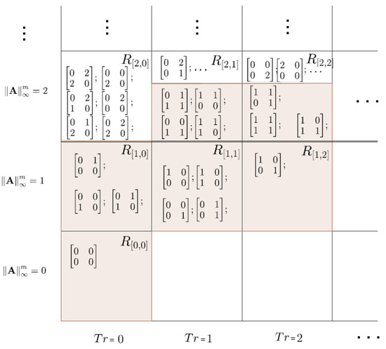
The upper approximation, i.e., the set , is in Figure 1 visualized as the union of all squares which include some coloured parts. The lower approximation, i.e., the set , is the union of all square which are fully coloured.
Figure 1.
The lower and upper approximation with relationfor matrices.
Theorem 6.
Let and be invertible hypergroups in , where is defined by for , , with relation . Then there is
where n is the size of the matrix.
Proof.
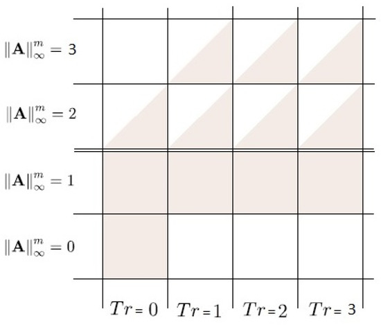
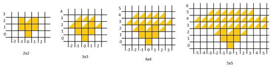
For the proof we use the idea of Example 7 and Figure 1, in which the lower approximation is the union of all squares which are fully coloured while the upper approximation is the union of all squares which contain some coloured parts. Notice that in Figure 1 rows indicate matrices with the same row norm (counted from the bottom) while columns (counted from the left) indicate matrices with the same trace. When one realizes how such a scheme in constructed, the proof becomes obvious. Indeed, take e.g., and focus on Figure 2 and (9).
□
Figure 2.
The lower and upper approximation with relation , for matrices .
Remark 3.
Note that the boundary, defined as the difference between the upper and the lower approximation, expands across the universe so that it has only two classes for and 7 classes for and 14 classes for and 23 classes for , i.e., classes for an matrix. Also, the upper approximation has classes and the lower approximation has classes. All these formulas can be easily seen in Figure 1 and Figure 2.
In what follows, we will consider and , where . In this way the construction can be considered as a dynamic system, where the set X is the hyperoperproduct defined by (5).
Corollary 2.
For there is . Moreover,
Now we will use the relation to present some basic and natural properties of the lower and upper approximations with respect to the above mentioned theorem. Recall that matrices are generators of the cyclic hypergroup .
Theorem 7.
The following properties hold:
- (1)
- (2)
- (3)
Recall that when defining the relation in (7) we used the row norm and trace. Let us now modify the definition to make use of the row norm and determinant. We define:
If we use the relation instead of , Figure 1 changes to Figure 3. This results in the following theorem.
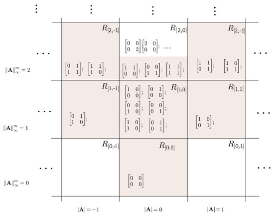
Figure 3.
The lower and upper approximation with relation for matrices .
Theorem 8.
Let and be invertible hypergroups in , where is defined by for , with relation . Than there is
where n is the size of the matrix.
Proof.
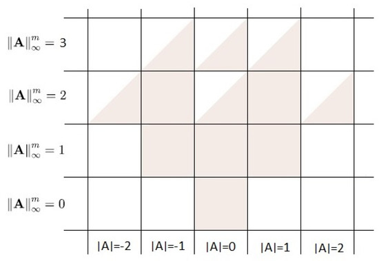
We use Figure 3 and Figure 4 in the proof. For an arbitrary size of the matrix, n, the lower approximation always consists of 6 classes of equivalence. Obviously, for an arbitrary n and there exists only one matrix (the null one), which is in , see the coloured square. For norm equal to 1, the proof is again obvious because thanks to the norm in every matrix of size n there can be maximum one 1 in every row, which means that the determinant of such a matrix can only be , 0 or 1. For norm 2 there exists, for an arbitrary size n a matrix with element 2 and zero determinant. Also, there exists a matrix which has one row with two 1’s. If we repeat such a row, the determinant is zero, see the partially coloured square. At the same time no matrix with 2 as an entry can be in a class with norm 2 and determinant 1 oe because in that case the respective row must contain only zeros as other entries. If we now expand the determinant with respect to that row, the calculation will include , where s is a subdeterminant and , which means that the determinant can never be 1 or . For norm 3 we get that the numbers of matrices can include 2 and 1, which means that the calculation of the determinant will include a difference, i.e., we can get an arbitrary number. In other words, for norm greater than 2 we cannot obtain fully coloured squares, i.e., classes of equivalence which consist only of matrices with entries 0 and 1. □
Figure 4.
The lower and upper approximation with relation for matrices .
Finding a general rule for the upper approximation when using the determinant is not as easy as it may seem. Even though it seems that the whole universum “behaves accordingly”, it is not easy to find an algorithm which would easily define the upper approximation. Therefore we at least include a theorem which shows an important property of the upper approximation. At the same time, its proof describes the upper approximation for .
Theorem 9.
For , and , the following holds:
Proof.
For the proof we use Figure 3 and Figure 5. Results for and , which had been computed by software means, are included below. □
Figure 5.
The lower and upper approximation with relation for matrices –.
Application in the Control Theory
Application of rough set theory is widely used in information technologies. This approach has fundamental importance in knowledge acquisition, cognitive science, pattern recognition, machine learning, database systems, etc. Rough sets are also used in sensors mapping in robotics.
If we examine how an autonomous mobile robot can get from point A to point B, we realize that it must have information about obstacles in front of itself to avoid collision. To find this out it uses sensors, mostly camera and LIDAR (an abbreviation of “Light Detection And Ranging”) for environment mapping [25,26].
We can easily find surjective function from a set of matrices (our model) to coordinates , where . These are coordinates of occupancy grid [26] cells (robotics usage), which must meet the following condition:
where are real coordinates that represents the interval/size of the cells in occupancy grid (see Figure 6). This process is called quantization. We can mark the occupancy grid as equivalence classes.
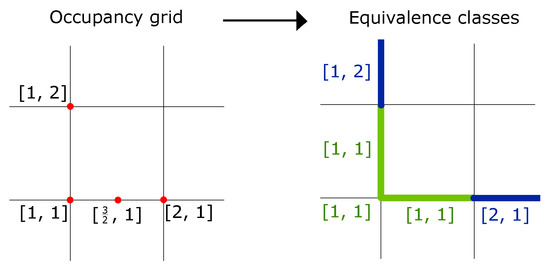
Figure 6.
Quantization from real coordinates to equivalence classes.
Both sensors can be attached to specific places on the top of robot. (Notice that all visualised information from sensors what we are working with are projected from 3D to 2D plane because of assumption that the robot can move only in 2 directions.) In our figures (for , for example) the lower approximation describes the robot’s shape and pose. We can be sure for occupation of these cells because of the fusion of sensor data with the known relative position between the sensors and the robot (its shape) in particular. As we can see, this approximation will never change depending on change of n (matrix size). This lower approximation is typical for an industrial warehouse robot.
Next part of LIDAR/camera scan is the upper approximation. This gives us information about all cells which were hit by the sensors. However, we can only say that these cells are occupied with probability between 0 and 1 (never 0 or 1) because this is how all current sensor work. The bigger the n, the bigger the range of sensors. Notice that the sensor scanning angle is symmetric by vertical axis of the sensor.
The above example makes use of a single sensor scan. However, we can process these scans into a whole simple mapping algorithm described in [12,26] or improved algorithm via particle filter described in [27].
5. Conclusions
In our paper we deal with a construction of cyclic hypergroups and present their links to rough sets. We construct subsets of such hypergroups which determine the approximation for finding the lower and upper approximation of the rough set. For this we use various types of equivalence relations. In our paper we choose the input of the matrix subhypergroups out of a two element set. Generalizing our results for arbitrary more-element sets is a topic of our further research. The constructions of the lower and upper approximation described in this paper for various n are very interesting, which can be, in case of norm and trace and , visualised in a simple figure; see Figure 7. Further research can also focus on finding the approximation set. For this we can look for inspiration in the intersection of the principal end and beginning of the hyperoperation in [10]. As a result we can form an approximation set which need not include the origin of the universe, i.e., .
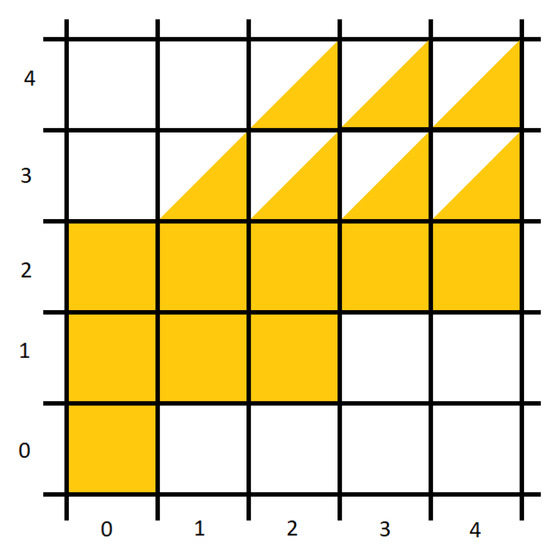
Figure 7.
The lower and upper approximation with relation for matrices and .
Author Contributions
Investigation, Š.K. and J.V.; Methodology, Š.K. and J.V.; Software, Š.K. and J.V.; Supervision, Š.K. and J.V.; Writing—original draft, Š.K. and J.V.; Writing—review & editing,Š.K. and J.V. All authors have read and agreed to the published version of the manuscript.
Funding
The first author was supported by the Ministry of Education, Youth and Sports within the National Sustainability Program I, project of Transport R&D Centre (LO1610) and the second author was supported by the FEKT-S-17-4225 grant of Brno University of Technology.
Conflicts of Interest
The authors declare no conflict of interest.
References
- Zadeh, L.A. Fuzzy sets. Inf. Control 1965, 8, 338–353. [Google Scholar] [CrossRef]
- Pavlak, Z. Rough Set: Theorerical Aspects of Reasoning Above Data; Kluver Academic Publishers: Dordrecht, The Netherlands, 1991. [Google Scholar]
- Pavlak, Z. Rough set. Int. J. Comput. Inf. Sci. 1982, 11, 341–356. [Google Scholar]
- Molodtsov, D. Soft set—First results. Comp. Math. Appl. 1999, 37, 19–31. [Google Scholar] [CrossRef]
- Chvalina, J. Functional Graphs, Quasi-ordered Sets and Commutative Hypergroups; Masaryk University: Brno, Czech Republic, 1995. (In Czech) [Google Scholar]
- Hošková, Š.; Chvalina, J.; Račková, P. Transposition hypergroups of Fredholm integral operators and related hyperstructures. Part I. J. Basic Sci. 2008, 4, 43–54. [Google Scholar]
- Novák, M. On EL-semihypergroups. Eur. J. Combin. 2015, 44 Pt B, 274–286. [Google Scholar]
- Novák, M.; Cristea, I. Composition in EL-hyperstructures. Hacet. J. Math. Stat. 2019, 48, 45–58. [Google Scholar] [CrossRef]
- Novák, M.; Křehlík, Š. EL-hyperstructures revisited. Soft Comput. 2018, 22, 7269–7280. [Google Scholar]
- Křehlík, Š.; Novák, M. From lattices to Hv-matrices. An. Şt. Univ. Ovidius Constanţa 2016, 24, 209–222. [Google Scholar] [CrossRef]
- Leoreanu-Foneta, V. The lower and upper approximation in hypergroup. Inf. Sci. 2008, 178, 3605–3615. [Google Scholar]
- Novák, M.; Křehlík, Š.; Staněk, D. n-ary Cartesian composition of automata. Soft Comput. 2019. [Google Scholar] [CrossRef]
- Novák, M.; Ovaliadis, K.; Křehlík, Š. A hyperstructure of Underwater Wireless Sensor Network (UWSN) design. In AIP Conference Proceedings 1978, Proceedings of the International Conference on Numerical Analysis and Applied Mathematics (ICNAAM 2017), The MET Hotel, Thessaloniki, Greece, 25–30 September 2017; American Institute of Physics: Thessaloniki, Greece, 2018. [Google Scholar]
- Račková, P. Hypergroups of symmetric matrices. In Proceedings of the 10th International Congress of Algebraic Hyperstructures and Applications (AHA 2008), Brno, Czech Republic, 3–9 September 2008; University of Defence: Brno, Czech Republic, 2009; pp. 267–272. [Google Scholar]
- Novák, M.; Křehlík, Š.; Cristea, I. Cyclicity in EL-hypergroups. Symmetry 2018, 10, 611. [Google Scholar] [CrossRef]
- Vougiouklis, T. Cyclicity in a Special Class of Hypergroups. Acta Universitatis Carolinae Mathematica Physica 1981, 22, 3–6. [Google Scholar]
- Skowron, A.; Dutta, S. Rough sets: Past, present, and future. Nat. Comput. 2018, 17, 855–876. [Google Scholar] [CrossRef] [PubMed]
- Anvariyeh, S.M.; Mirvakili, S.; Davvaz, B. Pavlak’s approximations in Γ-semihypergroups. Comput. Math. Appl. 2010, 60, 45–53. [Google Scholar] [CrossRef]
- Leoreanu-Foneta, V. Approximations in hypergroups and fuzzy hypergroups. Comput. Math. Appl. 2011, 61, 2734–2741. [Google Scholar] [CrossRef]
- Corsini, P.; Leoreanu, V. Applications of Hyperstructure Theory; Kluwer Academic Publishers: Dodrecht, The Netherlands; Boston, MA, USA; London, UK, 2003. [Google Scholar]
- Davvaz, B.; Leoreanu–Fotea, V. Applications of Hyperring Theory; International Academic Press: Palm Harbor, FL, USA, 2007. [Google Scholar]
- Vougiouklis, T. Hyperstructures and Their Representations; Hadronic Press: Palm Harbor, FL, USA, 1994. [Google Scholar]
- Chvalina, J.; Křehlík, Š.; Novák, M. Cartesian composition and the problem of generalising the MAC condition to quasi-multiautomata. An. Şt. Univ. Ovidius Constanţa 2016, 24, 79–100. [Google Scholar]
- Massouros, C.G. On the semi-sub-hypergroups of a hypergroup. Int. J. Math. Math. Sci. 1991, 14, 293–304. [Google Scholar] [CrossRef]
- Kokovkina, V.A.; Antipov, V.A.; Kirnos, V.P.; Priorov, A.L. The Algorithm of EKF-SLAM Using Laser Scanning System and Fisheye Camera. In Proceedings of the 2019 Systems of Signal Synchronization, Generating and Processing in Telecommunications (SYNCHROINFO), Yaroslavl, Russia, 1–3 July 2019; pp. 1–6. [Google Scholar]
- Vu, T.-D.; Aycard, O.; Appenrodt, N. Online Localization and Mapping with Moving Object Tracking in Dynamic Outdoor Environments. In Proceedings of the 2007 IEEE Intelligent Vehicles Symposium, Istanbul, Turkey, 13–15 June 2007; pp. 190–195. [Google Scholar]
- Zhu, D.; Sun, X.; Wang, L.; Liu, B.; Ji, K. Mobile Robot SLAM Algorithm Based on Improved Firefly Particle Filter. In Proceedings of the 2019 International Conference on Robots & Intelligent System (ICRIS), Haikou, China, 15–16 June 2019; pp. 35–38. [Google Scholar]
© 2019 by the authors. Licensee MDPI, Basel, Switzerland. This article is an open access article distributed under the terms and conditions of the Creative Commons Attribution (CC BY) license (http://creativecommons.org/licenses/by/4.0/).