Figure 1.
Geometry of the problem.
Figure 1.
Geometry of the problem.
Figure 2.
The h-curve for (a) velocity profile, (b) temperature profile when
Figure 2.
The h-curve for (a) velocity profile, (b) temperature profile when
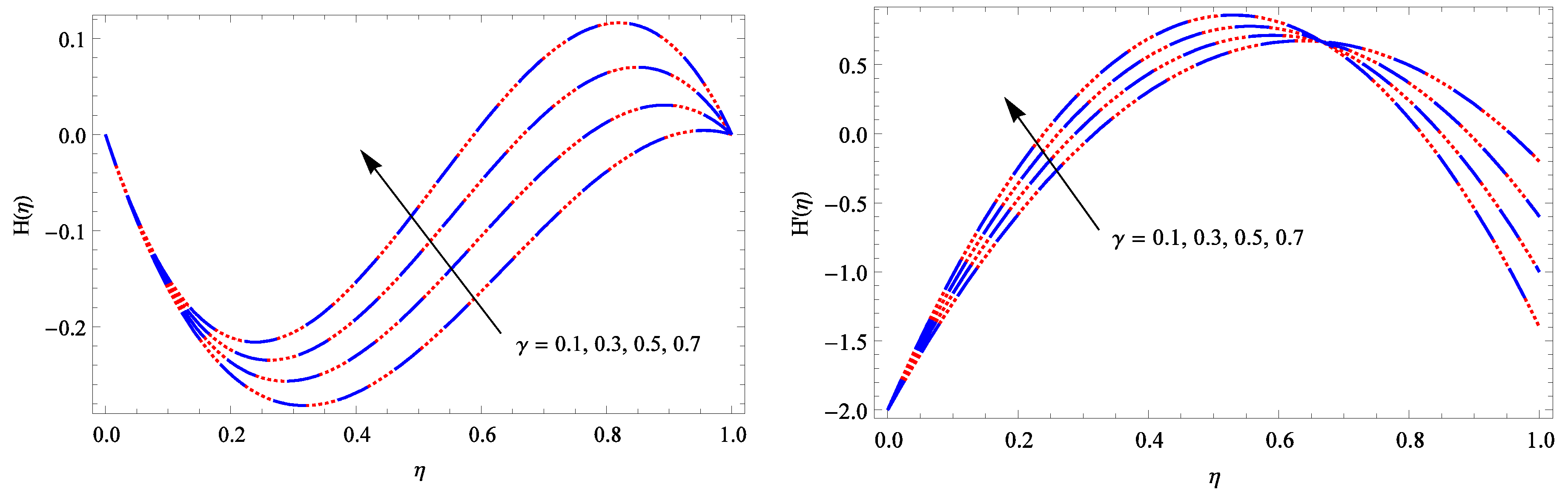
Figure 3.
Comparison of velocity components
and
for different values of stretching parameter
, dotted red lines represents the HAM solution while blue lines denotes the solution by Gorder et al. [
21].
Figure 3.
Comparison of velocity components
and
for different values of stretching parameter
, dotted red lines represents the HAM solution while blue lines denotes the solution by Gorder et al. [
21].
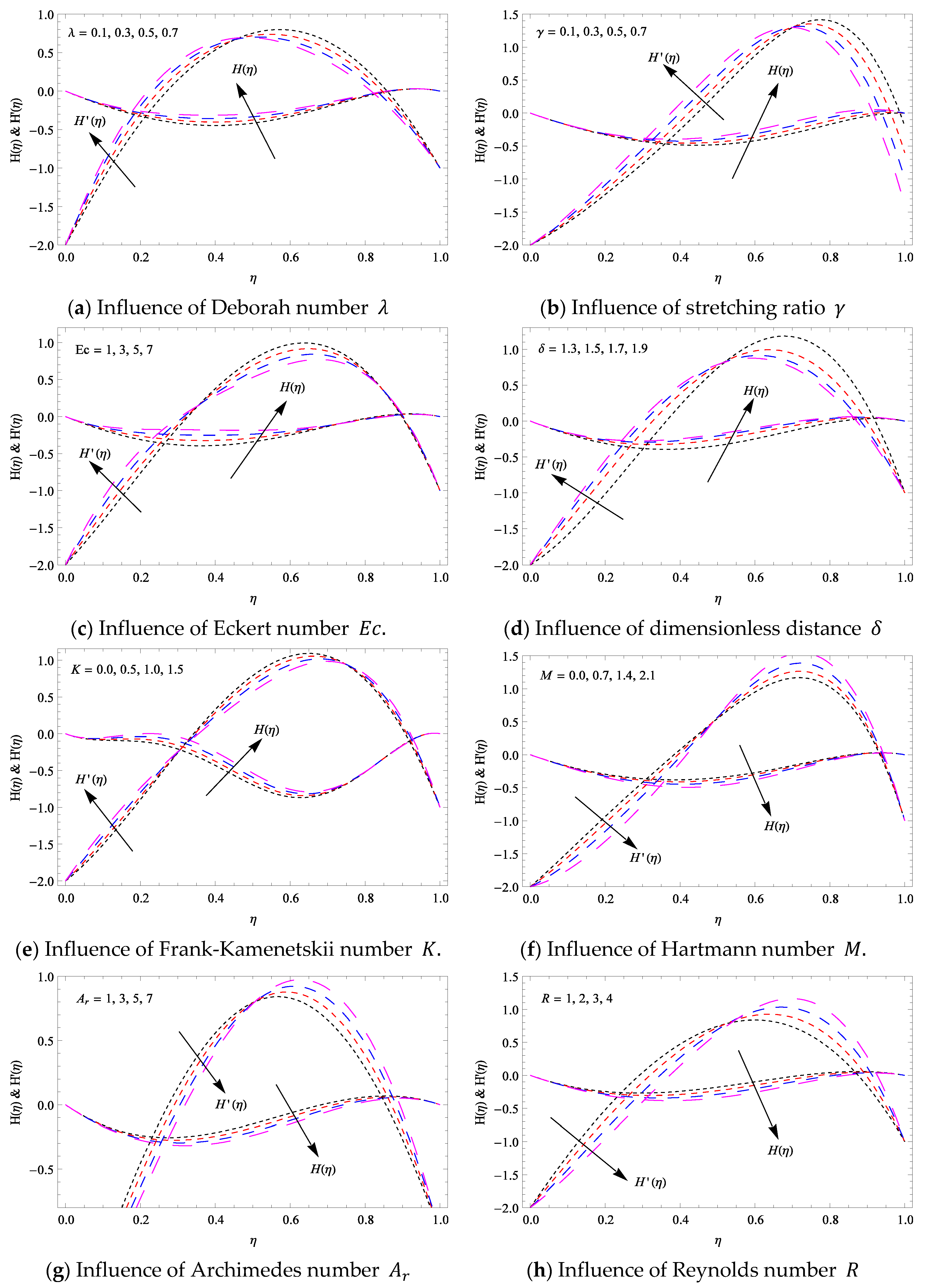
Figure 4.
In r and z components of velocities when and
Figure 4.
In r and z components of velocities when and
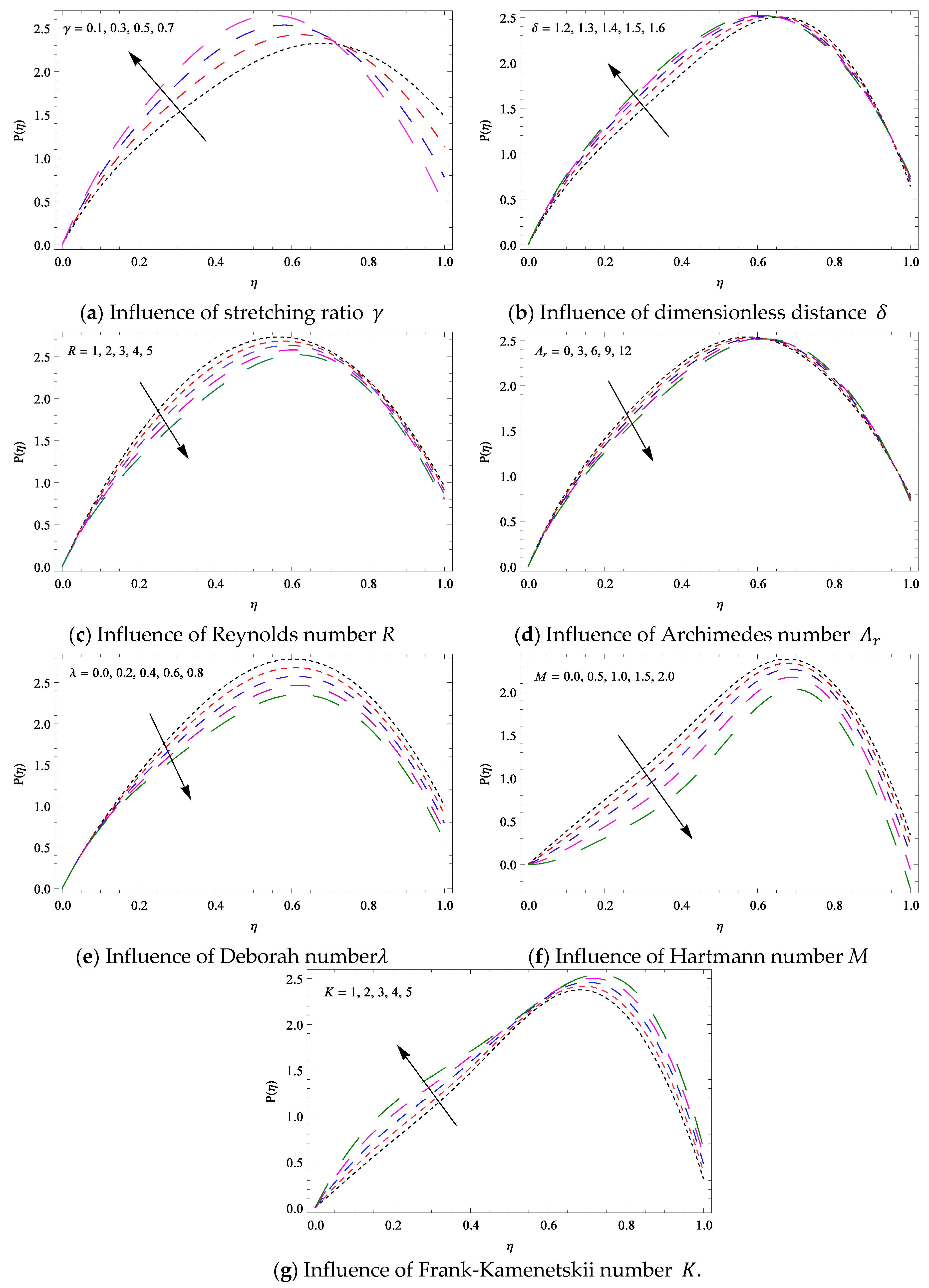
Figure 5.
Pressure distribution for different parameters with and .
Figure 5.
Pressure distribution for different parameters with and .
Figure 6.
Temperature profile for and .
Figure 6.
Temperature profile for and .
Figure 7.
(a–c) The in skin friction coefficients at both disks for various values of and with and
Figure 7.
(a–c) The in skin friction coefficients at both disks for various values of and with and
Figure 8.
(a,b) The variation in Nusselt number at both disks for various values of and when and .
Figure 8.
(a,b) The variation in Nusselt number at both disks for various values of and when and .
Table 1.
The convergence analysis of the homotopic solution with and
Table 1.
The convergence analysis of the homotopic solution with and
| Order of Approximation | | |
|---|
| 11 | 9.79594 | −1.91738 |
| 14 | 9.79619 | −1.91686 |
| 16 | 9.79643 | −1.91634 |
| 18 | 9.79667 | −1.91582 |
| 20 | 9.79717 | −1.91461 |
| 25 | 9.79717 | −1.91461 |
| 30 | 9.79717 | −1.91461 |
Table 2.
Comparison of for different values of with and
Table 2.
Comparison of for different values of with and
| Gorder et al. [21] | Present Result (HAM) |
|---|
| | | |
|---|
| 0.0 | 0.000 | −2.00 | 0.000 | −2.00 |
| 0.2 | −0.224 | −0.360 | −0.224 | −0.360 |
| 0.4 | −0.192 | 0.560 | −0.192 | 0.560 |
| 0.6 | −0.048 | 0.760 | −0.048 | 0.760 |
| 0.8 | 0.064 | 0.240 | 0.064 | 0.240 |
| 1.0 | 0.000 | −1.00 | 0.000 | −1.000 |
Table 3.
Numerical variation in wall shear stress at both surfaces of moving disk.
Table 3.
Numerical variation in wall shear stress at both surfaces of moving disk.
| | | | | | | | | | | | Lower Disk | Upper Disk |
|---|
| 0.2 | 01 | 05 | 1.0 | 1.0 | 0.2 | 0.5 | 0.5 | 0.5 | 02 | 2.0 | 0.1 | −116.204 | −252.335 |
| 0.4 | 01 | 05 | 1.0 | 1.0 | 0.2 | 0.5 | 0.5 | 0.5 | 02 | 2.0 | 0.1 | −129.404 | −262.989 |
| 0.6 | 01 | 05 | 1.0 | 1.0 | 0.2 | 0.5 | 0.5 | 0.5 | 02 | 2.0 | 0.1 | −142.249 | −272.563 |
| 0.5 | 1.0 | 05 | 1.0 | 1.0 | 0.2 | 0.5 | 0.5 | 0.5 | 02 | 2.0 | 0.1 | −135.869 | −267.915 |
| 0.5 | 1.5 | 05 | 1.0 | 1.0 | 0.2 | 0.5 | 0.5 | 0.5 | 02 | 2.0 | 0.1 | −149.413 | −273.824 |
| 0.5 | 2.0 | 05 | 1.0 | 1.0 | 0.2 | 0.5 | 0.5 | 0.5 | 02 | 2.0 | 0.1 | −162.905 | −281.867 |
| 0.5 | 01 | 1.0 | 1.0 | 1.0 | 0.2 | 0.5 | 0.5 | 0.5 | 02 | 2.0 | 0.1 | −1.63619 | −38.7856 |
| 0.5 | 01 | 2.0 | 1.0 | 1.0 | 0.2 | 0.5 | 0.5 | 0.5 | 02 | 2.0 | 0.1 | −22.2454 | −67.5845 |
| 0.5 | 01 | 3.0 | 1.0 | 1.0 | 0.2 | 0.5 | 0.5 | 0.5 | 02 | 2.0 | 0.1 | −44.9617 | −108.970 |
| 0.5 | 01 | 05 | 1.0 | 1.0 | 0.2 | 0.5 | 0.5 | 0.5 | 02 | 2.0 | 0.1 | −135.869 | −267.915 |
| 0.5 | 01 | 05 | 2.0 | 1.0 | 0.2 | 0.5 | 0.5 | 0.5 | 02 | 2.0 | 0.1 | −102.816 | −437.258 |
| 0.5 | 01 | 05 | 3.0 | 1.0 | 0.2 | 0.5 | 0.5 | 0.5 | 02 | 2.0 | 0.1 | −69.7624 | −606.601 |
| 0.5 | 01 | 05 | 1.0 | 1.0 | 0.2 | 0.5 | 0.5 | 0.5 | 02 | 2.0 | 0.1 | −135.869 | −267.915 |
| 0.5 | 01 | 05 | 1.0 | 1.5 | 0.2 | 0.5 | 0.5 | 0.5 | 02 | 2.0 | 0.1 | 115.683 | −430.368 |
| 0.5 | 01 | 05 | 1.0 | 2.0 | 0.2 | 0.5 | 0.5 | 0.5 | 02 | 2.0 | 0.1 | 367.236 | −592.821 |
| 0.5 | 01 | 05 | 1.0 | 1.0 | 0.2 | 0.5 | 0.5 | 0.5 | 02 | 2.0 | 0.1 | −135.869 | −267.915 |
| 0.5 | 01 | 05 | 1.0 | 1.0 | 0.4 | 0.5 | 0.5 | 0.5 | 02 | 2.0 | 0.1 | −195.891 | −369.982 |
| 0.5 | 01 | 05 | 1.0 | 1.0 | 0.6 | 0.5 | 0.5 | 0.5 | 02 | 2.0 | 0.1 | −255.476 | −472.018 |
| 0.5 | 01 | 05 | 1.0 | 1.0 | 0.2 | 0.5 | 0.5 | 0.5 | 02 | 2.0 | 0.1 | −135.869 | −267.915 |
| 0.5 | 01 | 05 | 1.0 | 1.0 | 0.2 | 0.6 | 0.5 | 0.5 | 02 | 2.0 | 0.1 | −62.2384 | −77.8090 |
| 0.5 | 01 | 05 | 1.0 | 1.0 | 0.2 | 0.7 | 0.5 | 0.5 | 02 | 2.0 | 0.1 | −23.2608 | −44.7235 |
| 0.5 | 01 | 05 | 1.0 | 1.0 | 0.2 | 0.5 | 0.1 | 0.5 | 02 | 2.0 | 0.1 | −130.344 | −270.583 |
| 0.5 | 01 | 05 | 1.0 | 1.0 | 0.2 | 0.5 | 0.3 | 0.5 | 02 | 2.0 | 0.1 | −133.108 | −269.244 |
| 0.5 | 01 | 05 | 1.0 | 1.0 | 0.2 | 0.5 | 0.5 | 0.5 | 02 | 2.0 | 0.1 | −135.869 | −267.915 |
| 0.5 | 01 | 05 | 1.0 | 1.0 | 0.2 | 0.5 | 0.5 | 0.1 | 02 | 2.0 | 0.1 | −14.4518 | −37.1367 |
| 0.5 | 01 | 05 | 1.0 | 1.0 | 0.2 | 0.5 | 0.5 | 0.3 | 02 | 2.0 | 0.1 | −52.1849 | −61.3395 |
| 0.5 | 01 | 05 | 1.0 | 1.0 | 0.2 | 0.5 | 0.5 | 0.5 | 02 | 2.0 | 0.1 | −89.1381 | −99.7870 |
| 0.5 | 01 | 05 | 1.0 | 1.0 | 0.2 | 0.5 | 0.5 | 0.5 | 3.5 | 2.0 | 0.1 | 24.7854 | −1205.14 |
| 0.5 | 01 | 05 | 1.0 | 1.0 | 0.2 | 0.5 | 0.5 | 0.5 | 4.0 | 2.0 | 0.1 | 195.575 | −1786.25 |
| 0.5 | 01 | 05 | 1.0 | 1.0 | 0.2 | 0.5 | 0.5 | 0.5 | 4.5 | 2.0 | 0.1 | 445.195 | −2541.17 |
| 0.5 | 01 | 05 | 1.0 | 1.0 | 0.2 | 0.5 | 0.5 | 0.5 | 02 | 2.0 | 0.1 | −135.869 | −267.915 |
| 0.5 | 01 | 05 | 1.0 | 1.0 | 0.2 | 0.5 | 0.5 | 0.5 | 02 | 2.3 | 0.1 | −185.374 | −345.966 |
| 0.5 | 01 | 05 | 1.0 | 1.0 | 0.2 | 0.5 | 0.5 | 0.5 | 02 | 2.6 | 0.1 | −247.552 | −440.297 |
| 0.5 | 01 | 05 | 1.0 | 1.0 | 0.2 | 0.5 | 0.5 | 0.5 | 02 | 2.0 | 0.1 | −155.783 | −257.838 |
| 0.5 | 01 | 05 | 1.0 | 1.0 | 0.2 | 0.5 | 0.5 | 0.5 | 02 | 2.0 | 0.2 | −154.907 | −257.367 |
| 0.5 | 01 | 05 | 1.0 | 1.0 | 0.2 | 0.5 | 0.5 | 0.5 | 02 | 2.0 | 0.3 | −154.003 | −256.903 |
Table 4.
Numerical variation in local Nusselt number at both surfaces of moving disk.
Table 4.
Numerical variation in local Nusselt number at both surfaces of moving disk.
| | | | | | | | | | | | Lower Disk | Upper Disk |
|---|
| 0.2 | 01 | 05 | 1.0 | 1.0 | 0.2 | 0.5 | 0.5 | 0.5 | 02 | 2.0 | 0.1 | −43.2173 | 62.2902 |
| 0.4 | 01 | 05 | 1.0 | 1.0 | 0.2 | 0.5 | 0.5 | 0.5 | 02 | 2.0 | 0.1 | −43.1456 | 64.2379 |
| 0.6 | 01 | 05 | 1.0 | 1.0 | 0.2 | 0.5 | 0.5 | 0.5 | 02 | 2.0 | 0.1 | −43.1225 | 66.2978 |
| 0.5 | 1.0 | 05 | 1.0 | 1.0 | 0.2 | 0.5 | 0.5 | 0.5 | 02 | 2.0 | 0.1 | −43.1714 | 65.2526 |
| 0.5 | 1.5 | 05 | 1.0 | 1.0 | 0.2 | 0.5 | 0.5 | 0.5 | 02 | 2.0 | 0.1 | −49.2164 | 71.3174 |
| 0.5 | 2.0 | 05 | 1.0 | 1.0 | 0.2 | 0.5 | 0.5 | 0.5 | 02 | 2.0 | 0.1 | −55.2913 | 77.3855 |
| 0.5 | 01 | 2.0 | 1.0 | 1.0 | 0.2 | 0.5 | 0.5 | 0.5 | 02 | 2.0 | 0.1 | −1.93260 | 10.9702 |
| 0.5 | 01 | 3.0 | 1.0 | 1.0 | 0.2 | 0.5 | 0.5 | 0.5 | 02 | 2.0 | 0.1 | −9.76591 | 20.5937 |
| 0.5 | 01 | 4.0 | 1.0 | 1.0 | 0.2 | 0.5 | 0.5 | 0.5 | 02 | 2.0 | 0.1 | −20.8434 | 35.8615 |
| 0.5 | 01 | 05 | 1.0 | 1.0 | 0.2 | 0.5 | 0.5 | 0.5 | 02 | 2.0 | 0.1 | −34.5174 | 58.1590 |
| 0.5 | 01 | 05 | 2.0 | 1.0 | 0.2 | 0.5 | 0.5 | 0.5 | 02 | 2.0 | 0.1 | −59.2591 | 126.626 |
| 0.5 | 01 | 05 | 3.0 | 1.0 | 0.2 | 0.5 | 0.5 | 0.5 | 02 | 2.0 | 0.1 | −70.4176 | 209.251 |
| 0.5 | 01 | 05 | 1.0 | 1.0 | 0.2 | 0.5 | 0.5 | 0.5 | 02 | 2.0 | 0.1 | −34.5174 | 58.1590 |
| 0.5 | 01 | 05 | 1.0 | 1.5 | 0.2 | 0.5 | 0.5 | 0.5 | 02 | 2.0 | 0.1 | −65.0929 | 88.3373 |
| 0.5 | 01 | 05 | 1.0 | 2.0 | 0.2 | 0.5 | 0.5 | 0.5 | 02 | 2.0 | 0.1 | −95.5317 | 118.241 |
| 0.5 | 01 | 05 | 1.0 | 1.0 | 0.2 | 0.5 | 0.5 | 0.5 | 02 | 2.0 | 0.1 | −37.1562 | 59.1911 |
| 0.5 | 01 | 05 | 1.0 | 1.0 | 0.4 | 0.5 | 0.5 | 0.5 | 02 | 2.0 | 0.1 | −35.3967 | 58.5028 |
| 0.5 | 01 | 05 | 1.0 | 1.0 | 0.6 | 0.5 | 0.5 | 0.5 | 02 | 2.0 | 0.1 | −33.6384 | 57.8153 |
| 0.5 | 01 | 05 | 1.0 | 1.0 | 0.2 | 0.5 | 0.5 | 0.5 | 02 | 2.0 | 0.1 | −34.5174 | 58.1590 |
| 0.5 | 01 | 05 | 1.0 | 1.0 | 0.2 | 0.6 | 0.5 | 0.5 | 02 | 2.0 | 0.1 | −4.57816 | 17.6285 |
| 0.5 | 01 | 05 | 1.0 | 1.0 | 0.2 | 0.7 | 0.5 | 0.5 | 02 | 2.0 | 0.1 | −2.16759 | 8.23666 |
| 0.5 | 01 | 05 | 1.0 | 1.0 | 0.2 | 0.5 | 0.1 | 0.5 | 02 | 2.0 | 0.1 | −32.5620 | 56.3592 |
| 0.5 | 01 | 05 | 1.0 | 1.0 | 0.2 | 0.5 | 0.3 | 0.5 | 02 | 2.0 | 0.1 | −33.5476 | 57.2673 |
| 0.5 | 01 | 05 | 1.0 | 1.0 | 0.2 | 0.5 | 0.5 | 0.5 | 02 | 2.0 | 0.1 | −34.5174 | 58.1590 |
| 0.5 | 01 | 05 | 1.0 | 1.0 | 0.2 | 0.5 | 0.5 | 0.1 | 02 | 1.0 | 0.1 | −4.03154 | 4.78376 |
| 0.5 | 01 | 05 | 1.0 | 1.0 | 0.2 | 0.5 | 0.5 | 0.3 | 02 | 1.0 | 0.1 | −7.31547 | 21.5100 |
| 0.5 | 01 | 05 | 1.0 | 1.0 | 0.2 | 0.5 | 0.5 | 0.5 | 02 | 1.0 | 0.1 | −34.5174 | 58.1590 |
| 0.5 | 01 | 05 | 1.0 | 1.0 | 0.2 | 0.5 | 0.5 | 0.5 | 3.5 | 1.0 | 0.1 | −128.255 | 180.574 |
| 0.5 | 01 | 05 | 1.0 | 1.0 | 0.2 | 0.5 | 0.5 | 0.5 | 4.0 | 1.0 | 0.1 | −171.887 | 236.943 |
| 0.5 | 01 | 05 | 1.0 | 1.0 | 0.2 | 0.5 | 0.5 | 0.5 | 4.5 | 1.0 | 0.1 | −221.713 | 301.095 |
| 0.5 | 01 | 05 | 1.0 | 1.0 | 0.2 | 0.5 | 0.5 | 0.5 | 02 | 2.0 | 0.1 | −34.5174 | 58.1590 |
| 0.5 | 01 | 05 | 1.0 | 1.0 | 0.2 | 0.5 | 0.5 | 0.5 | 02 | 2.3 | 0.1 | −43.9555 | 76.6222 |
| 0.5 | 01 | 05 | 1.0 | 1.0 | 0.2 | 0.5 | 0.5 | 0.5 | 02 | 2.6 | 0.1 | −53.7965 | 97.8575 |
| 0.5 | 01 | 05 | 1.0 | 1.0 | 0.2 | 0.5 | 0.5 | 0.5 | 02 | 1.0 | 0.1 | −35.1337 | 58.7998 |
| 0.5 | 01 | 05 | 1.0 | 1.0 | 0.2 | 0.5 | 0.5 | 0.5 | 02 | 1.0 | 0.2 | −35.8183 | 59.5099 |
| 0.5 | 01 | 05 | 1.0 | 1.0 | 0.2 | 0.5 | 0.5 | 0.5 | 02 | 1.0 | 0.3 | −36.5027 | 60.2180 |
Table 5.
The numerical values of Critical Frank–Kamenetskii number for various parameters.
Table 5.
The numerical values of Critical Frank–Kamenetskii number for various parameters.
| | | | | | | | | | | |
|---|
| 0.3 | 01 | 05 | 01 | 01 | 0.5 | 0.5 | 0.01 | 02 | 2.0 | 1.2 | −10.8144 |
| 0.5 | 01 | 05 | 01 | 01 | 0.5 | 0.5 | 0.01 | 02 | 2.0 | 1.2 | −10.8151 |
| 0.7 | 01 | 05 | 01 | 01 | 0.5 | 0.5 | 0.01 | 02 | 2.0 | 1.2 | −10.8170 |
| 0.5 | 01 | 05 | 01 | 01 | 0.5 | 0.5 | 0.01 | 02 | 2.0 | 1.2 | −10.8151 |
| 0.5 | 03 | 05 | 01 | 01 | 0.5 | 0.5 | 0.01 | 02 | 2.0 | 1.2 | −10.7897 |
| 0.5 | 05 | 05 | 01 | 01 | 0.5 | 0.5 | 0.01 | 02 | 2.0 | 1.2 | −10.7400 |
| 0.5 | 01 | 01 | 01 | 01 | 0.5 | 0.5 | 0.01 | 02 | 2.0 | 1.2 | −10.6770 |
| 0.5 | 01 | 02 | 01 | 01 | 0.5 | 0.5 | 0.01 | 02 | 2.0 | 1.2 | −10.6946 |
| 0.5 | 01 | 03 | 01 | 01 | 0.5 | 0.5 | 0.01 | 02 | 2.0 | 1.2 | −10.7235 |
| 0.5 | 01 | 05 | 01 | 01 | 0.5 | 0.5 | 0.01 | 02 | 2.0 | 1.2 | −10.8151 |
| 0.5 | 01 | 05 | 02 | 01 | 0.5 | 0.5 | 0.01 | 02 | 2.0 | 1.2 | −10.9559 |
| 0.5 | 01 | 05 | 03 | 01 | 0.5 | 0.5 | 0.01 | 02 | 2.0 | 1.2 | −11.0960 |
| 0.5 | 01 | 05 | 01 | 01 | 0.5 | 0.5 | 0.01 | 02 | 2.0 | 1.2 | −10.8151 |
| 0.5 | 01 | 05 | 01 | 02 | 0.5 | 0.5 | 0.01 | 02 | 2.0 | 1.2 | −10.8064 |
| 0.5 | 01 | 05 | 01 | 03 | 0.5 | 0.5 | 0.01 | 02 | 2.0 | 1.2 | −10.7978 |
| 0.5 | 01 | 05 | 01 | 01 | 2.0 | 0.5 | 0.01 | 02 | 2.0 | 1.2 | −10.5643 |
| 0.5 | 01 | 05 | 01 | 01 | 2.5 | 0.5 | 0.01 | 02 | 2.0 | 1.2 | −10.4735 |
| 0.5 | 01 | 05 | 01 | 01 | 3.0 | 0.5 | 0.01 | 02 | 2.0 | 1.2 | −10.3631 |
| 0.5 | 01 | 05 | 01 | 01 | 0.5 | 0.3 | 0.01 | 02 | 2.0 | 1.2 | −10.6729 |
| 0.5 | 01 | 05 | 01 | 01 | 0.5 | 0.5 | 0.01 | 02 | 2.0 | 1.2 | −10.8151 |
| 0.5 | 01 | 05 | 01 | 01 | 0.5 | 0.7 | 0.01 | 02 | 2.0 | 1.2 | −10.9575 |
| 0.5 | 01 | 05 | 01 | 01 | 0.5 | 0.5 | 0.1 | 02 | 2.0 | 1.2 | −12.1179 |
| 0.5 | 01 | 05 | 01 | 01 | 0.5 | 0.5 | 0.2 | 02 | 2.0 | 1.2 | −14.0721 |
| 0.5 | 01 | 05 | 01 | 01 | 0.5 | 0.5 | 0.3 | 02 | 2.0 | 1.2 | −16.1551 |
| 0.5 | 01 | 05 | 01 | 01 | 0.5 | 0.5 | 0.01 | 10 | 2.0 | 1.2 | −11.3132 |
| 0.5 | 01 | 05 | 01 | 01 | 0.5 | 0.5 | 0.01 | 50 | 2.0 | 1.2 | −15.1132 |
| 0.5 | 01 | 05 | 01 | 01 | 0.5 | 0.5 | 0.01 | 100 | 2.0 | 1.2 | −20.1335 |
| 0.5 | 01 | 05 | 01 | 01 | 0.5 | 0.5 | 0.01 | 02 | 01 | 1.2 | −10.4104 |
| 0.5 | 01 | 05 | 01 | 01 | 0.5 | 0.5 | 0.01 | 02 | 02 | 1.2 | −10.3151 |
| 0.5 | 01 | 05 | 01 | 01 | 0.5 | 0.5 | 0.01 | 02 | 03 | 1.2 | −11.2584 |
| 0.5 | 01 | 05 | 01 | 01 | 0.5 | 0.5 | 0.01 | 02 | 2.0 | 0.5 | −10.8071 |
| 0.5 | 01 | 05 | 01 | 01 | 0.5 | 0.5 | 0.01 | 02 | 2.0 | 1.0 | −10.8127 |
| 0.5 | 01 | 05 | 01 | 01 | 0.5 | 0.5 | 0.01 | 02 | 2.0 | 1.5 | −10.8189 |


 ,
, 


