Serious Solutions for Unsteady Axisymmetric Flow over a Rotating Stretchable Disk with Deceleration

Department of Mathematics, DCC-KFUPM, KFUPM Box 5084, Dhahran 31261, Saudi Arabia
Symmetry 2020, 12(1), 96; https://doi.org/10.3390/sym12010096
Submission received: 12 December 2019
/
Revised: 2 January 2020
/
Accepted: 2 January 2020
/
Published: 3 January 2020
(This article belongs to the Special Issue Recent Advances in Mathematical Aspect in Engineering)
Abstract
:In this article, the author has examined the unsteady flow over a rotating stretchable disk with deceleration. The highly nonlinear partial differential equations of viscous fluid are simplified by existing similarity transformation. Reduced nonlinear ordinary differential equations are solved by homotopy analysis method (HAM). The convergence of HAM solutions is also obtained. A comparison table between analytical solutions and numerical solutions is also presented. Finally, the results for useful parameters, i.e., disk stretching parameters and unsteadiness parameters, are found.
1. Introduction
Recently, due to the massive practical application in the scientific and technical field, the study of the rotating stretchable disk has become significant, such as thermal power generation system, medical equipment’s, computer storage devices, rotating machinery, gas turbine routers, air cleaning machines, crystal growth process, and in aerodynamic applications [1]. Initially, von Kármán [2] conducted a study on rotating disk. Several researchers then illustrated the different aspects of this important analysis. Fang and Zhang [3] have highlighted the flow between two stretchable disks and found the exact solutions. The parameters analysis and optimization of entropy generation in unsteady magneto hydrodynamics flow over a rotating stretchable flow over a rotating disk using artificial neural network and practical swarm optimization algorithm was presented by Rashidi et al. [4]. Recently, Fang and Tao [5] wrote about the unsteady flow over a rotating stretchable disk with deceleration. After using the similarity analysis, they found the numerical solutions.
In many situations, exact solutions are very difficult and in most of the cases exact solutions are impossible. Therefore, series solutions are more useful if they satisfy the given initial and boundary value problems. Nevertheless, there are various analytical approaches, and each approach has certain limitations. However, homotopy analysis method (HAM) has many advantages over many analytical methods. Liao [6] introduced the idea of HAM, which is used by many researchers effectively. Some useful studies are cited in [7,8,9,10,11,12,13,14,15]. The purpose of this article is to illustrate the application of HAM for unsteady Newtonian fluid flow over a rotating stretchable disk with declaration. Tables provide a correlation between current HAM solution and Fang and Tao’s [5] numerical solution.
2. Formulation of the Problem
Let us consider an incompressible, laminar, and unsteady flow of a viscous fluid or Newtonian fluid over a stretchable disk, which is rotating about the -axis with time dependent angular velocity , where is constant angular speed of the disk and ‘b’ is the measure of unsteadiness. Flow is due to the rotation of the stretchable disk and is axisymmetric about the z-axis. Figure 1 describe the geometry of the proposed problem. The governing equations for an unsteady three-dimensional flow of viscous fluid in cylindrical coordinates are shown below.
where is along the radial direction, is along the azimuthal direction, and is in normal direction to the axis. Here, Equation (1) is the continuity equation and Equations (2) and (4) represent the momentum equation for incompressible flow.
Where , and are the velocities along directions, is the density of fluid, is the pressure, is the kinematic viscosity, and are the stress which are defined as
The proposed boundary conditions are specified in accordance with the geometry of the problem as
where ‘a’ is the disk stretching parameter.
Introducing, the similarity transformation used in [5] are
Applying these similarities into the above equations, following non-dimensional equations along with boundary conditions can be obtained as
where is the unsteadiness parameter.
3. Homotopy Analysis Method
Homotopy Analysis Method (HAM) [6,7,8,9,10,11,12,13,14,15] is used to find an analytical solution to Equations (8) and (11). The velocity distribution and can be expressed by a set of base functions
in the form
in which and are the coefficients, the initial guesses can be selected on the basis of the law of the solution expressions and of the boundary conditions:
The auxiliary linear operators are
which satisfy
where are integral constants.
3.1. Zeroth-Order Deformation Equation
If denote an embedding parameter, and indicate the non zero auxiliary parameters for and , the zeroth-order deformations for the given problem are
Defining the nonlinear operators for the above problem as
For and , one can have
By Taylor’s theorem
and
3.2. Mth-Order Deformation
Differentiating the zeorth-order deformation Equations (21) and (23) with respect to , then setting , and finally dividing them by , the mth-order deformation equations can be obtained as
where
in which and denote the special solutions of Equations (32) and (33) and the integral constants are calculated by the (34) boundary conditions. Equations (32) and (34) can be solved using Mathematica for = 1, 2, 3….
4. Convergence of the HAM Solution
The homotopy analysis method includes the regulating parameter , which controls the region of convergence and HAM solution approximation. To ensure that the solutions converge within the admissible spectrum of auxiliary parameter values and and , were sketched for 15th-order approximation. The are plotted in Figure 2 and Figure 3. The admissible ranges of values of and are these ranges vary with the change in parameters.
5. Results and Discussion
To solve Equations (8) and (9) homotopy analysis method (HAM) is applied as a subject to the boundary conditions (11). Homotopy analysis method is a strong analytical technique which is applied to obtain the convergent series solution of nonlinear differential equations. The convergence region for HAM through are sketched and analyzed in Figure 3 and Figure 4. Homotopy analysis method provides great freedom to obtain the convergent result. The convergence region varies for different values of and . Table 1, Table 2, Table 3 and Table 4 represent the convergence of solution for different values of parameters. The error analysis of the obtained approximated results is as follows.
where is the residual error of Equations (8) and (9) at the mth-order approximation. It is observed that 10th-order approximation is in good agreement with the numerical result.
The convergence control parameter plays an important role. In Table 5 and Table 6, the effect of on convergence is shown. Table 5 and Table 6 show that the convergence of the solution depends strongly on . It can be seen easily that for one set of the convergence is faster than the other.
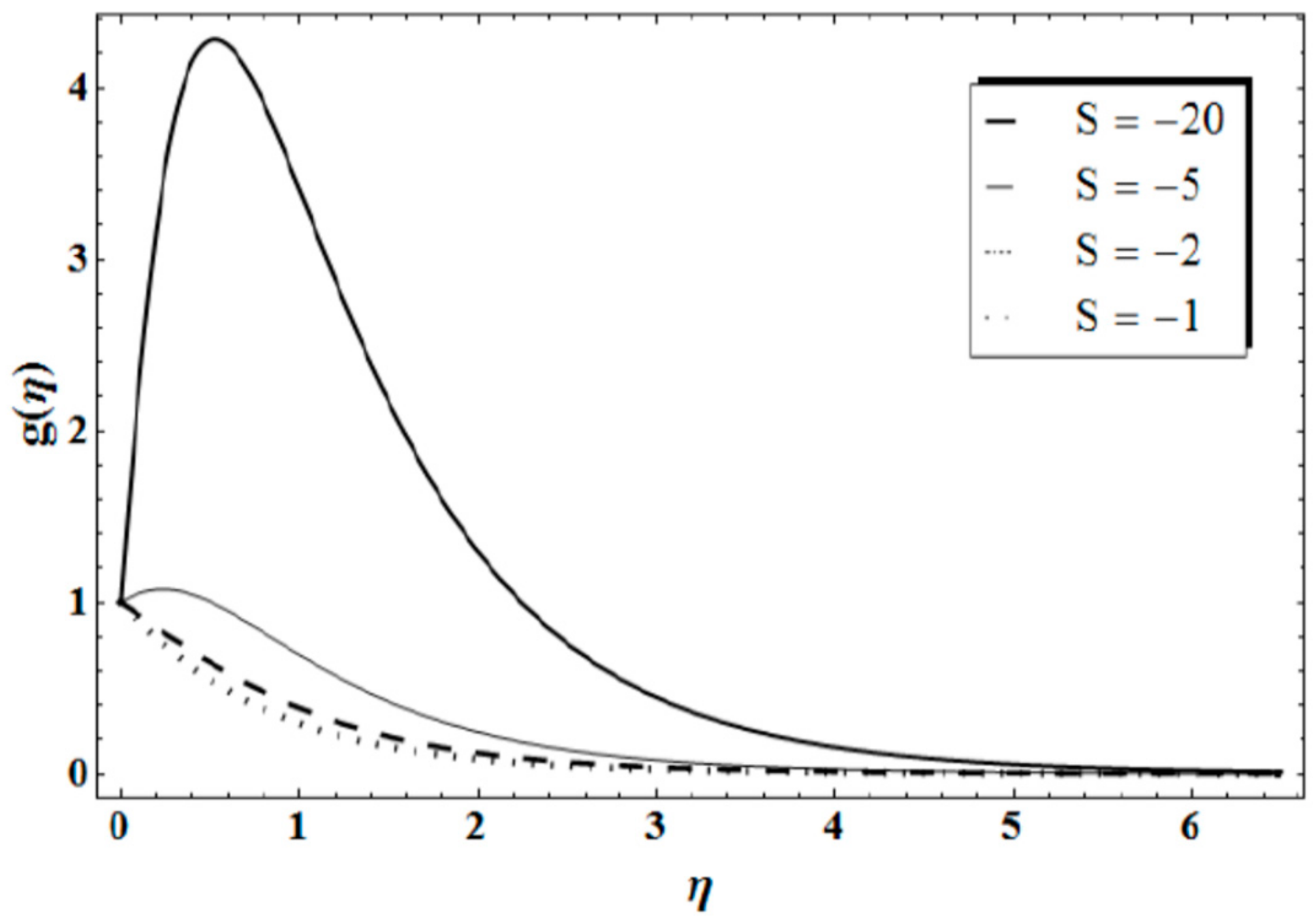
In Figure 5 and Figure 6, the comparison of 5th-order approximation with 10th-order approximation is shown, which again provide the facts for convergence. The Mathematica software is used to compute the results for higher-order approximation. As the given problem is highly nonlinear, the computation time increases if higher-order approximation is computed or increases the value of the parameters. For and , the given problem becomes a special case as mentioned in the numerical paper [5]. Table 7 provides the convergence result for this special case as well. The results obtained in the present research for this special case are also in very good agreement with the numerical result. This shows the strength of homotopy analysis methods. It is found that for small , decreases with the increase of ‘a’ as shown in Table 2 and Table 3. Figure 7 represents the velocity distribution for different values of . It is observed that with the increase in disk stretching parameter the velocity decreases. Figure 8 and Figure 9 show that with the decrease in the unsteadiness parameter, both tangential and radial velocities increase.
6. Conclusions
In this research, viscous axisymmetric flow is studied on a stretchable rotating disk with deceleration. It is found that Navier–Stokes equation admits a similarity solution, which depends on non-dimensionalized parameters and measuring unsteadiness and disk stretching, respectively. The resulting group of nonlinear ordinary differential equations is then solved analytically using homotopy analysis method (HAM). In numerical paper [5] it is mentioned that there are two solution branches. The upper solution branch is physically feasible, but the lower solution branch may not be practically possible. Here, the author has discussed and evaluated the outcome for a physical solution from the upper field.
The main results are summarized as
- Results obtained by homotopy analysis method are in good agreement with existing numerical results;
- All the velocity profiles decrease with an increase in unsteadiness parameter ;
- Radial and axial velocity of the flow increases with the increase in disk stretching parameter , whereas tangential velocity shows a decreasing trend with an increase in ;
- Variation trend decays with faster velocity to the ambient for fast deceleration as compared to the slow deceleration of the disk.
Funding
This research received funding from KFUPM.
Acknowledgments
The author wishes to express his thanks for the support received from King Fahd University of Petroleum and Minerals.
Conflicts of Interest
Author declare no conflicts of interest with any one.
References
- Turkyilmazoglu, M. Three-dimensional MHD stagnation flow due to a stretchable rotating disk. Int. J. Heat Mass Transf. 2012, 55, 6959–6965. [Google Scholar] [CrossRef]
- Von Kármán, T. Über Laminar Und Turbulente Reibung. J. Appl. Math. Mech. 1921, 1, 233–252. [Google Scholar]
- Fang, T.; Zhang, J. Flow between two stretchable disks-An exact solution of the NavierStokes equations. Int. Commun. Heat Mass Transf. 2008, 35, 892–895. [Google Scholar] [CrossRef]
- Rashidi, M.M.; Ali, M.; Freidoonimehr, N.; Nazari, F. Parametric analysis and optimization of entropy generation in unsteady MHD flow over a stretching rotating disk using articial neural network and particle swarm optimization algorithm. Energy 2013, 55, 1–14. [Google Scholar] [CrossRef]
- Fang, T.; Hua, T. Unsteady viscous flow over a rotating stretchable disk with deceleration. Commun. Nonlinear Sci. Numer. Simul. 2012, 17, 5064–5072. [Google Scholar] [CrossRef]
- Liao, S. On the homotopy analysis method for nonlinear problems. Appl. Math. Comput. 2004, 147, 499–513. [Google Scholar] [CrossRef]
- Nadeem, S.; Awais, M. Thin film flow of an unsteady shrinking sheet through porous medium with variable viscosity. Phys. Lett. A 2008, 372, 4965–4972. [Google Scholar] [CrossRef]
- Nadeem, S.; Ali, M. Analytical solutions for pipe flow of a fourth grade fluid with Reynold and Vogel’s models of viscosities. Commun. Nonlinear Sci. Numer. Simul. 2009, 14, 2073–2090. [Google Scholar] [CrossRef]
- Nadeem, S.; Abbasbandy, S.; Hussain, M. Series solutions of boundary layer flow of a Micropolar fluid near the stagnation point towards a shrinking sheet. Z. Fur Nat. 2009, 64, 575–582. [Google Scholar] [CrossRef]
- Nadeem, S. Thin film flow of a third grade fluid with variable viscosity. Z. Fur Nat. 2009, 64, 553–558. [Google Scholar] [CrossRef]
- Nadeem, S.; Hussain, A. MHD flow of a viscous fluid on a non-linear porous shrinking sheet by Homotopy analysis method. Appl. Math. Mech. 2009, 30, 1569–1578. [Google Scholar] [CrossRef]
- Khan, H.; Ram, N.M.; Vajravelu, K.; Liao, S.J. The explicit Series Solution of SIR and SIS Epidemic Models. Appl. Math. Comput. 2009, 215, 653–669. [Google Scholar] [CrossRef]
- Khan, H.; Liao, S.J.; Ram, N.M.; Vajravelu, K. An analytical solution for a nonlinear time delay model in Biology. Commun. Nonlinear Sci. Numer. Simul. 2009, 14, 3141–3148. [Google Scholar] [CrossRef]
- Khan, H.; Xu, H. Series Solution of Thomas Fermi Atom Model. Phys. Lett. A 2007, 365, 111–115. [Google Scholar] [CrossRef]
- Liao, S. A short review on the homotopy analysis method in fluid mechanics. J. Hydrodyn. 2010, 22, 882–884. [Google Scholar] [CrossRef]
Figure 1.
Geometry of the problem.

Figure 2.
15th-order for .
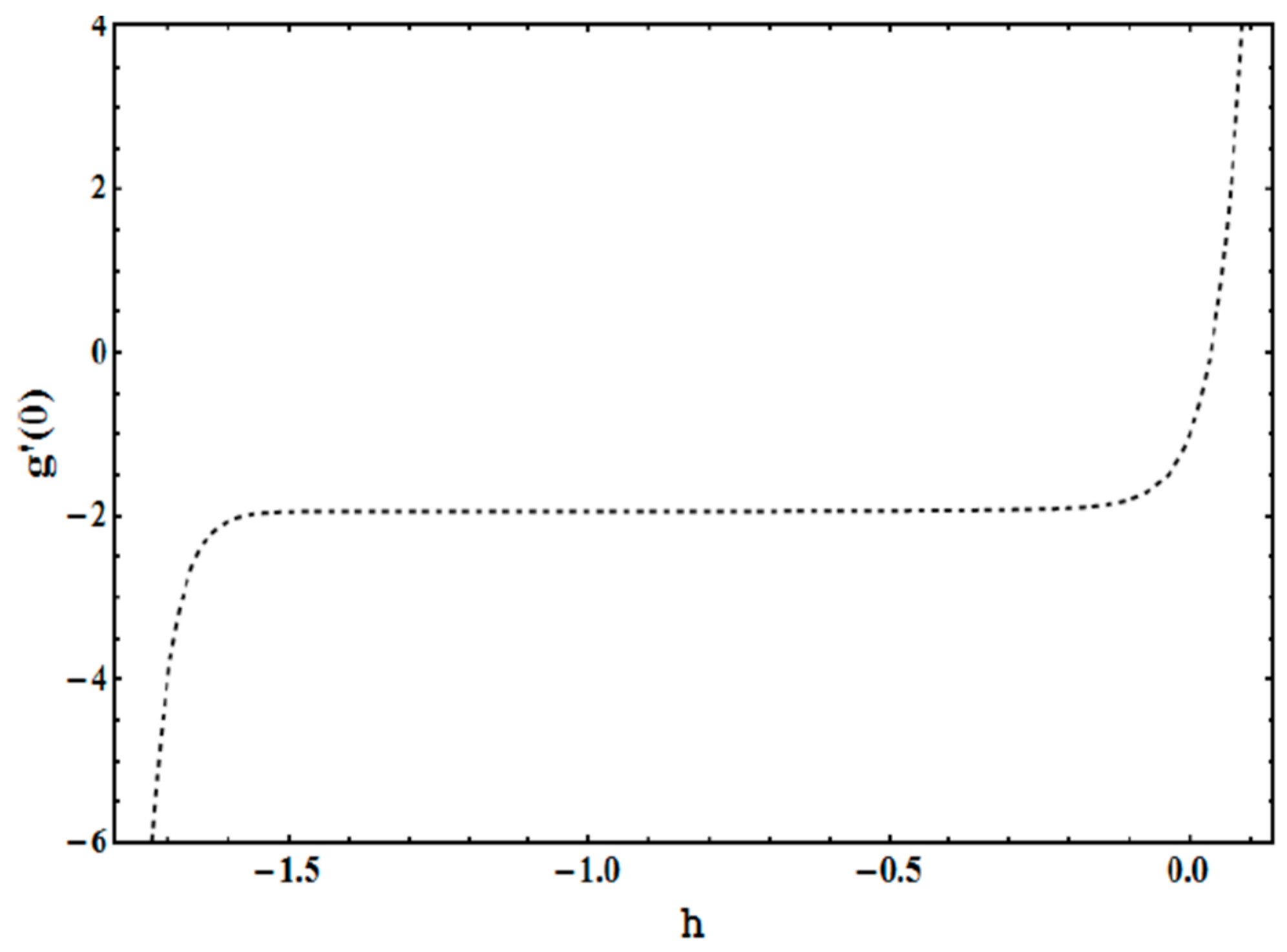
Figure 3.
15th-order for .

Figure 4.
Comparison of convergence of (line: 10th-order, dots: 5th-order).

Figure 5.
Comparison of convergence of (line: 10th-order, dots: 5th-order).

Figure 6.
For solid line: , Dashed line: 10th order HAM approximation for .

Figure 7.
For 10th-order HAM approximation for .

Figure 8.
Variation of for different values of unsteadiness parameter for .
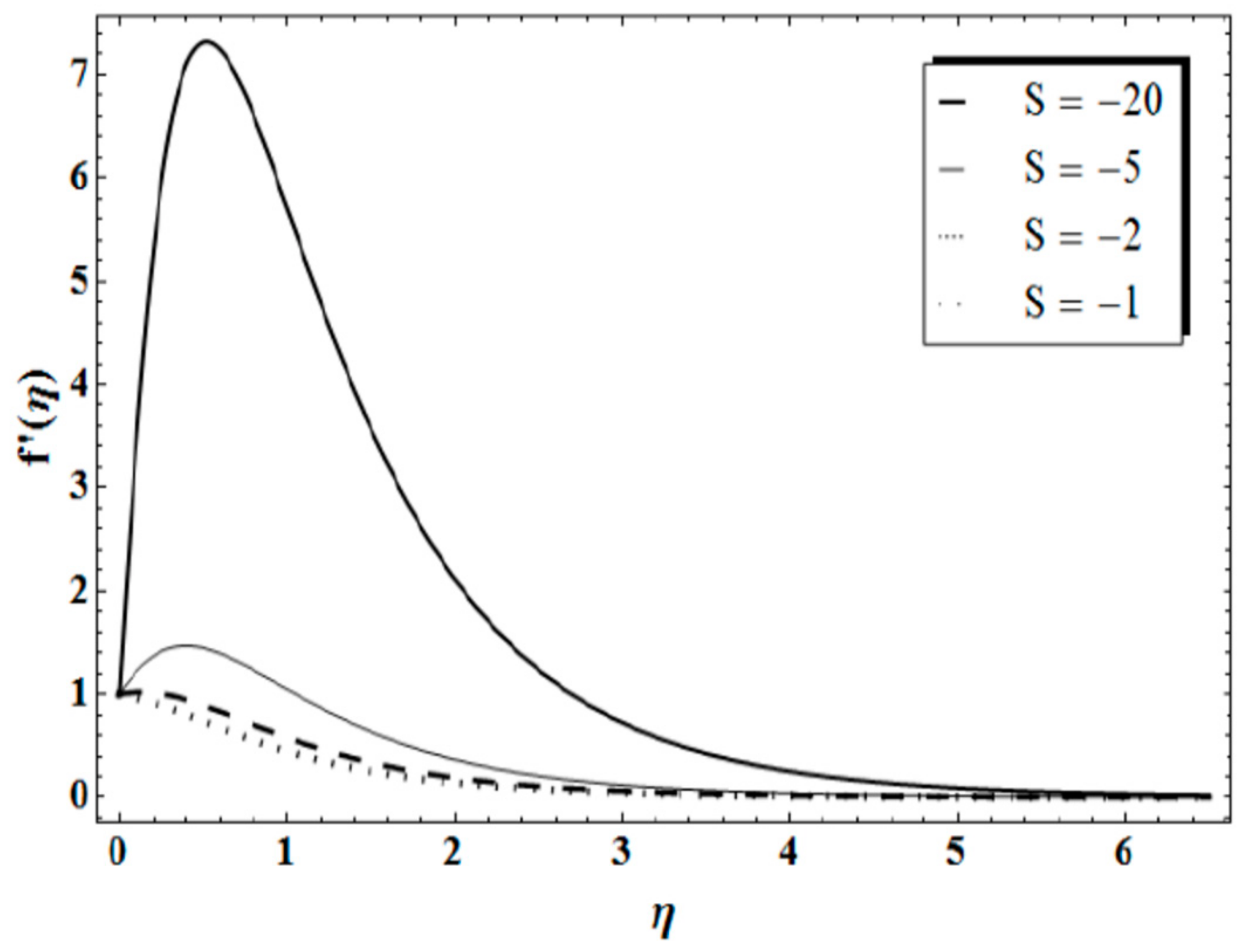
Figure 9.
Variation of for different values of unsteadiness parameter for .

Table 1.
Comparison of the numerical result [5] with homotopy analysis method (HAM) convergent result when .
Table 1.
Comparison of the numerical result [5] with homotopy analysis method (HAM) convergent result when .
| Order | ||||
|---|---|---|---|---|
| 2nd | −0.7673 | −1.196 | 0.311 | 0.044 |
| 4th | −0.6945 | −1.246 | 0.021 | 0.0067 |
| 6th | −0.6681 | −1.264 | 0.0046 | 0.0021 |
| 8th | −0.6581 | −1.270 | 0.00091 | 0.000715 |
| 10th | −0.6543 | −1.271 | 0.00014 | 0.00023 |
Numerical result [5] .
Table 2.
Comparison of the numerical result [5] with HAM convergent result when .
Table 2.
Comparison of the numerical result [5] with HAM convergent result when .
| Order | ||||
|---|---|---|---|---|
| 2nd | −0.9642 | −1.3321 | 0.031 | 0.379 |
| 4th | −0.9374 | −1.4162 | 0.0047 | 0.0055 |
| 6th | −0.9262 | −1.446 | 0.00075 | 0.00091 |
| 8th | −0.9217 | −1.458 | 0.00012 | 0.00016 |
| 10th | −0.9200 | −1.4627 | 0.000018 | 0.000033 |
Numerical result [5] .
Table 3.
Comparison of the numerical result [5] with HAM convergent result when .
Table 3.
Comparison of the numerical result [5] with HAM convergent result when .
| Order | ||||
|---|---|---|---|---|
| 2nd | −2.779 | −1.658 | 0.408 | 0.543 |
| 4th | −2.9729 | −1.847 | 0.0876 | 0.136 |
| 6th | −3.044 | −1.924 | 0.0234 | 0.0437 |
| 8th | −3.072 | −1.953 | 0.0071 | 0.018 |
| 10th | −3.082 | −1.958 | 0.0024 | 0.012 |
Numerical result [5] .
Table 4.
Comparison of the numerical result [5] with HAM convergent result when .
Table 4.
Comparison of the numerical result [5] with HAM convergent result when .
| Order | ||||
|---|---|---|---|---|
| 2nd | −0.9062 | −1.2760 | 0.1051 | 0.0221 |
| 4th | −0.8592 | −1.3424 | 0.0283 | 0.0037 |
| 6th | −0.8319 | −1.3654 | 0.0077 | 0.00082 |
| 8th | −0.8172 | −1.3741 | 0.0021 | 0.00021 |
| 10th | −0.8093 | −1.3774 | 0.00058 | 0.00006 |
Numerical result [5] .
Table 5.
The Convergence analysis of for different when and .
| Order | Err | Err | ||
|---|---|---|---|---|
| 2nd | −0.9007 | 0.1062 | −0.9243 | 0.1405 |
| 4th | −0.8535 | 0.0283 | −0.8826 | 0.0514 |
| 6th | −0.8282 | 0.0076 | −0.8658 | 0.0312 |
| 8th | −0.8149 | 0.0021 | −0.8325 | 0.0069 |
| 10th | −0.8080 | 0.0005 | −0.8201 | 0.0025 |
Numerical result [5] .
Table 6.
The Convergence analysis of for different when and .
| Order | Err | Err | ||
|---|---|---|---|---|
| 2nd | −1.2345 | 0.03718 | −1.2786 | 0.022 |
| 4th | −1.3157 | 0.0087 | −1.3445 | 0.0036 |
| 6th | −1.3502 | 0.0024 | −1.3578 | 0.0016 |
| 8th | −1.366 | 0.0007 | −1.3737 | 0.00021 |
| 10th | −1.3734 | 0.0002 | −1.3768 | 0.00006 |
Numerical result [5] .
Table 7.
Comparison of the numerical result [5] with HAM convergent result for special case when analysis .
© 2020 by the author. Licensee MDPI, Basel, Switzerland. This article is an open access article distributed under the terms and conditions of the Creative Commons Attribution (CC BY) license (http://creativecommons.org/licenses/by/4.0/).
Share and Cite
MDPI and ACS Style
Sadiq, M.A. Serious Solutions for Unsteady Axisymmetric Flow over a Rotating Stretchable Disk with Deceleration. Symmetry 2020, 12, 96. https://doi.org/10.3390/sym12010096
AMA Style
Sadiq MA. Serious Solutions for Unsteady Axisymmetric Flow over a Rotating Stretchable Disk with Deceleration. Symmetry. 2020; 12(1):96. https://doi.org/10.3390/sym12010096
Chicago/Turabian StyleSadiq, Muhammad Adil. 2020. "Serious Solutions for Unsteady Axisymmetric Flow over a Rotating Stretchable Disk with Deceleration" Symmetry 12, no. 1: 96. https://doi.org/10.3390/sym12010096
Note that from the first issue of 2016, this journal uses article numbers instead of page numbers. See further details here.