Impact of Nonlinear Thermal Radiation on the Time-Dependent Flow of Non-Newtonian Nanoliquid over a Permeable Shrinking Surface

Abstract

Symmetry and fluid dynamics either advances the state-of-the-art of mathematical methods and extends the limitations of existing methodologies to new contributions in fluid. Physical scenario is modelled in terms of differential equations as mathematical models in fluid mechanics to address current challenges. In this work a physical problem to examine the unsteady flow of a third-grade non-Newtonian liquid induced through a permeable shrinking surface containing nanoliquid is considered. The model of Buongiorno is utilized comprising the thermophoresis and Brownian effects through nonlinear thermal radiation and convective condition. Based on the flow symmetry, suitable similarity transformations are employed to alter the partial differential equations into nonlinear ordinary differential equations and then these ordinary differential equations are numerically executed via three-stage Lobatto IIIa formula. The flow symmetry is discussed for interesting physical parameters and thus this work is concluded. More exactly, the impacts of pertinent constraints on the concentration, temperature and velocity profiles along together drag force, Sherwood and Nusselt numbers are explained through the aid of the tables and plots. The outcomes reveal that the dual nature of solutions is gained for a specific amount of suction and flow in the decelerating form $A<0$. However, the unique result is obtained for flow in accelerating form $A\ge 0$. In addition, the non-linear parameter declines the liquid velocity and augments the concentration and temperature fields in the first result, whereas the contrary behavior is scrutinized in the second result.

1. Introduction

In recent times, non-Newtonian liquids play an imperative role in industrial and engineering processes due to their numerous applications. Here, blood, paints, clay coatings, molten plastics, certain oils, artificial fibers, ketchup, etc., are a few examples. These liquids defy Newton′s law of viscosity due to their vital elastic properties. These kinds of liquids are found in an ample variety of realistic problems, enclosing essential significance in polymer depolarization, composite processing, boiling, bubble absorption, etc. Non-Newtonian liquids are scrutinized via three foremost classes, for instance, the integral type, differential type, and rate type. A third-grade liquid is a subclass liquid of the differential kind of model which can envisage the normal stresses along with the phenomena of shear thickening and thinning. Keçebaş and Yürüsoy [1] discussed the time-dependent flow of a special type of third-grade liquid and obtained the solution through similarity variables. Ellahi and Riaz [2] obtained an analytical result of the magnetohydrodynamics (MHD) flow of a third-grade liquid through erratic viscosity analysis. Sahoo and Do [3] explored the impact of the slip factor on a magnetic field comprising a third-grade liquid induced through a stretched sheet. The slip impact on a third-grade liquid from a stretched surface moving in exponential form was discussed by Sahoo and Poncet [4]. Abbasbandy and Hayat [5] discussed the special third-grade liquid through a permeable moving surface. Rahman et al. [6] inspected the mixed convective flow of a third-grade liquid close to a stagnation position from an exponentially stretching surface. Hussain et al. [7] presented solar radiation model for the magnetic field along with third-grade nanoliquid from a convectively heated stretched surface. Naganthran et al. [8] scrutinized the time-dependent flow of a special third-grade liquid through a porous stretched/shrinking surface. They observed the dual nature of results which remained true for the shrinking and stretched surfaces, and they also executed stability analysis. Recently, Reddy et al. [9] have inspected the time-dependent flow of a third-grade liquid through a cylinder. They found that a significant impact of third-grade fluid can observed in the flow field as compared to Newtonian fluid.

In recent times, the study of nanoliquids has gathered considerable curiosity, due to the field’s assorted realistic applications, including use in pharmaceutical medicines, thermal systems, electronics, nuclear reactors, chemical industry, etc. Nanoliquids are solid liquid particles which hold nanofiber or nanometer sized particles, having sizes of 1–100 nm, which are scattered in liquids such as water, lubricants, ethylene glycol, bio-fluids, oil, and polymer solutions. In recent times, it has been shown that nanoliquids demonstrate enhanced properties, including an enhanced thermophysical behavior, a modified viscosity, and enhanced thermal diffusivity, density, and thermal conductivity. A novel category of liquid has been described by Choi [10], which has been acknowledged as a nanoliquid. The phenomenon of the augmentation the thermal conductivity through dispersion of the nanomaterial in the liquid was shown by Masuda et al. [11]. Later, Buongiorno [12] observed that the motion of Brownian and thermophoretic diffusion of nanomaterials offers immense potential improvement in liquid thermal conductivity. As a result of these impacts, he recommended variations in situations of convective transport. This plays a significant role in several applications in various industries, like in the collection of aerosols, the safety of nuclear reactors, and eradicating tiny particles from gas streams. Khan and Pop [13] scrutinized flow involving a nanoliquid from a stretched surface using Buongiorno′s model. Then, Rana and Bhargava [14] expanded this problem through the use of a different geometry, namely, a non-linear stretched surface. The impact of the heat transport containing nanoliquid induced through a heated stretching surface was inspected through Makinde and Aziz [15]. The results revealed that the preserved thermal features were significantly distorted by escalating the impacts of thermophoresis and Brownian movement. Recently, several researchers [16,17,18,19,20] have discussed the importance of thermophoresis along with Brownian motion with different physical aspects.

The impact of thermal radiation through convective boundary circumstances is involved in numerous industrial and engineering processes, including gas turbines, the storage of thermal energy, die forging, nuclear turbines, and chemical reactions. Aziz [21] looked at the flow of a flat surface by employing a convective condition. Makinde and Aziz [22] scrutinized the magnetic impact of free and forced convective flow on the characteristic of heat transfer in an erect plate in a convective condition in a porous medium. The boundary layer flow provoked through a permeable stretched surface through a convective condition was scrutinized by Ishak [23]. Yao et al. [24] investigated flow with a permeable convectively heated shrinking and stretching wall and found an exact result. Rahman et al. [25] utilized the convective condition to find the solution numerically for mixed convective flow through an upright flat plate in a convective condition. Mustafa et al. [26] analyzed Maxwell liquid and an exponential stretched surface with a convective condition engrossed in a nanoliquid. Ibrahim and Haq [27] explored electrically conducting flow involving a nanoliquid from a stretched sheet in a convective condition. Makinde et al. [28] looked into the impact of MHD on flow comprising a nanoliquid through a connectivity-heated stretched sheet through radiation and slip impacts. The influence of convective condition on MHD flow with nonlinear radiation involving Carreau liquid induced by a stretched sheet was examined by Khan et al. [29]. Recently, Mabood and Khan [30] considered the impact of time-dependent flow with magnetic field from a stretched surface with convective condition.

However, time-dependent flow in the presence of a precise third-grade nanoliquid induced by a shrinking surface through nonlinear thermal radiation and a convective condition has not yet been explored. Although, the literature review has revealed that just a small amount of research has been carried out in a two-phase model comprising nanofluids in non-Newtonian fluid. Second, most researchers have found only one solution regarding the flow field. In addition, with a shrinking surface, a boundary layer flow through a shrinking surface is not achievable because the vorticity produced in this case is not confined inside the boundary layer. To maintain the structure of the boundary layer, the flow requires a certain value of exterior suction at the permeable sheet. Thus, we inspect the impact of nonlinear radiation on time-dependent flow through a shrinking surface involving a special third-grade nanofluid and obtain the dual solutions. The significant technique bvp4c (which is actually a finite difference technique which employs the 3-stage Lobatto IIIa formula) is utilized to solve transmuted ordinary differential equations (ODE’s). It is estimated that this study may be helpful for the examination of bundle and shrink wrappings, etc., and is a procedure through which manufactured goods or a group of goods may be wrapped in a movable cover or wrapper of plastic film, leading to the application of heat shrinkage and firmly conforming to the shape of the enclosed contents. The important aspect of this procedure is shrinking film. Owing to its real advantages, shrinking film has seen utilization in numerous industries at several stages of processes relating to packaging.

2. Formulation of the Problem

An unsteady nonlinear radiative flow, together with mass and heat transport, containing a special third-grade liquid induced through a permeable shrinking surface crammed by nanoliquids was developed. It is supposed that the x and y axes denote alongside the sheet and normal to it, respectively. The nanoliquid velocity of shrinking sheet is $ax/\left(1-ct\right)+u_w(x,t)=0$ with $a>0$ and $c$ showing the unsteadiness of the problem. In addition, the sheet was convectively heated by temperature $T_f$, which suggests a heat transport coefficient $h_f$. The considerations of the physical flow problem for third-grade liquids were considered as was considered by Fosdick and Rajagopal [31].

$${\mathrm{T}}_1+p\mathrm{I}=\mu {\mathrm{A}}_1+{\alpha }_1{\mathrm{A}}_2+{\alpha }_2{\mathrm{A}}_1^2+\beta \left({\mathrm{trA}}_1^2\right){\mathrm{A}}_1$$

(1)

where $\mu$, ${\mathrm{T}}_1$, $p$, and $\mathrm{I}$ represent the viscosity, Cauchy stress tensor, pressure, and identity tensor, respectively, and ${\alpha }_1$, ${\alpha }_2$, and $\beta$ represent the material moduli. Following Fosdick and Rajagopal [31], we imposed the following conditions:

$$0\le \mu , 0\le \beta , 0\le {\alpha }_1, {\left(24\mu \beta \right)}^{0.5}\ge \left|{\alpha }_1+{\alpha }_2\right|$$

(2)

Through these statements, the leading equations that oversee the time-dependent flow are presented as [4,8,26]:

$$\frac{\partial v}{\partial y}=-\frac{\partial u}{\partial x}$$

(3)

$$\frac{\partial u}{\partial t}+v\frac{\partial u}{\partial y}+u\frac{\partial u}{\partial x}-\nu \frac{{\partial }^{2}u}{\partial y^2}-6\kappa {\left(\frac{\partial u}{\partial y}\right)}^2\frac{{\partial }^{2}u}{\partial y^2}=0$$

(4)

$$\frac{\partial T}{\partial t}+v\frac{\partial T}{\partial y}+u\frac{\partial T}{\partial x}-\alpha \frac{{\partial }^{2}T}{\partial y^2}=\tau \left[\left(\frac{D_T}{T_{\infty }}\right){\left(\frac{\partial T}{\partial y}\right)}^2+D_B\frac{\partial C}{\partial y}\frac{\partial T}{\partial y}\right]-\frac{1}{{\left(\rho c_p\right)}_f}\frac{\partial q_r}{\partial y}$$

(5)

$$\frac{\partial C}{\partial t}+v\frac{\partial C}{\partial y}+u\frac{\partial C}{\partial x}-D_B\frac{{\partial }^{2}C}{\partial y^2}=\left(\frac{D_T}{T_{\infty }}\right)\left(\frac{\partial T^2}{\partial y^2}\right)$$

(6)

The boundary conditions are:

$$\begin{array}{ll}\hfill t<0:& C=C_{\infty }, v=0, u=0, T=T_{\infty } \mathrm{for} \mathrm{all} x,y,\hfill \\ \hfill t\ge 0:& C=C_w, v+v_w(t)=0, u-u_w(x,t)=0, -k\frac{\partial T}{\partial y}=h_f(t)\left(T_f-T\right) \mathrm{at} y=0,\hfill \\ & u\to 0, C\to C_{\infty }, T\to T_{\infty } \mathrm{as} y\to \infty .\hfill \end{array}$$

(7)

Here, $\left(v,u\right)$ denotes the components of velocity in the $y-,x-$ directions, respectively, $\alpha$, $\nu$ and $\rho$ denote the thermal diffusivity, kinematic viscosity, and density, respectively, $C$, $D_B$, $D_T$ and $\kappa$ denote the concentration of nanoparticles, the Brownian motion, thermophoresis diffusion coefficient, and the non-Newtonian parameter, respectively, and $\tau ={\left(\rho c_p\right)}_p/{\left(\rho c_p\right)}_f$ is the ratio of capacity.

In Equation (3), $q_r$ (radiative heat-flux) is presented as was obtained by Khan et al. [29]:

$$q_r=-\frac{\partial T^4}{\partial y}\frac{4{\sigma }^{*}}{3k^{*}}=-T^3\frac{\partial T}{\partial y}\frac{16{\sigma }^{*}}{3k^{*}},$$

(8)

where $\left(k^{*},{\sigma }^{*}\right)$ denotes the mean-absorption and the Stefan–Boltzmann constants, respectively. Utilizing Equation (8), Equation (5) became:

$$\frac{\partial T}{\partial t}+v\frac{\partial T}{\partial y}+u\frac{\partial T}{\partial x}-\tau \left[D_B\frac{\partial C}{\partial y}\frac{\partial T}{\partial y}+\left(\frac{D_T}{T_{\infty }}\right){\left(\frac{\partial T}{\partial y}\right)}^2\right]=\frac{\partial }{\partial y}\left[\left(\alpha +\frac{16{\sigma }^{*}{T}^3}{3{(\rho c_p)}_f{k}^{*}}\right)\frac{\partial T}{\partial y}\right]$$

(9)

Currently, we establish the similarity variables:

$$\eta =y\sqrt{\frac{a}{v\left(1-ct\right)}}, \psi =\sqrt{\frac{av}{\left(1-ct\right)}}xf(\eta ), \varphi (\eta )=\frac{C-C_{\infty }}{C_w-C_{\infty }}, \theta (\eta )=\frac{T-T_{\infty }}{T_f-T_{\infty }}.$$

(10)

Here $\eta$ and $\psi$ denote the similarity variable and the stream function, respectively, and we get $T=\left[T_{\infty }+T_{\infty }\left({\theta }_w-1\right)\theta \right]$ through ${\theta }_w>1$, where ${\theta }_w=T_f/T_{\infty }$ is the ratio of temperature. For the purpose of the similarity result, we presume that $\kappa ={\kappa }_0{\left(1-ct\right)}^3/x^2$, with ${\kappa }_0>0$ being a constant (see Naganthran et al. in [8]), $v_w(t)=v_0/\sqrt{1-ct}$ is the suction with $v_0>0$, and $h_f=d{\left(1-ct\right)}^{-0.5}$ with $d>0$ (see Mahapatra and Nandy in [32]).

Employing Equation (10), Equations (4)–(9) are transmuted into the ODE’s:

$$\left(1+K{f^{″}}^2\right)f^{‴}+f{f}^{″}-A\left(f^{\prime }+\frac{1}{2}\eta f^{″}\right)-{f^{\prime }}^2=0$$

(11)

$${\theta }^{″}+\mathrm{Pr}f{\theta }^{\prime }+\frac{4}{3R_d}\frac{d}{d\eta }\left[{\left\{1+\left({\theta }_w-1\right)\theta \right\}}^3{\theta }^{\prime }\right]-\frac{1}{2}\mathrm{Pr}A\eta {\theta }^{\prime }+\mathrm{Pr}\left[Nt{\left({\theta }^{\prime }\right)}^2+Nb{\theta }^{\prime }{\varphi }^{\prime }\right]=0$$

(12)

$${\varphi }^{″}+Lef{\varphi }^{\prime }+\frac{Nt}{Nb}{\theta }^{″}-\frac{1}{2}\mathrm{Pr}LeA\eta {\varphi }^{\prime }=0$$

(13)

Along with

$$\begin{array}{l}{f}^{\prime }(0)=-1, f(0)=S, {\theta }^{\prime }(0)=-\gamma \left(1-\theta (0)\right), \varphi (0)=1,\\ \varphi (\infty )\to 0, f^{\prime }(\infty )\to 0, \theta (\infty )\to 0,\end{array}$$

(14)

$$K=6{\kappa }_0{a}^3/{\nu }^2$$

$$\mathrm{Pr}=\nu /\alpha$$

$$A=-c/a$$

$$Nt=\tau D_T\left(T_f-T_{\infty }\right)/T_{\infty }\nu$$

$$\gamma =d\sqrt{\nu /a}/k$$

$$Nb=\tau D_B\left(C_w-C_{\infty }\right)/\nu$$

$$S=v_0/\sqrt{a\nu }>0$$

$$R_d=k{k}^{*}/4{\sigma }^{*}{T}_{\infty }^3$$

$$Le=\nu /D_B.$$

In above, K is the dimensionless non-Newtonian constraint, Pr is the Prandtl number, A is the unsteady constant, Nt is the thermophoresis, γ is the convective parameter, Nb is the Brownian motion, S is the suction, Rd id the thermal radiation and Le is the Lewis parameter.

The imperative engineering quantities of interest are the friction factor, heat, and mass transfer, which are presented as follows:

$$C_{fx}=\frac{{\tau }_w}{\rho u_w^2}, N{u}_x=-\frac{x{q}_w}{k(T_f-T_w)}, S{h}_x=\frac{x{m}_w}{D_B(C_w-C_{\infty })},$$

(15)

where $q_w$, $m_w$, and ${\tau }_w$ denote the shear stress, mass flux and heat flux, respectively, and are shown as follows:

$${\tau }_w=\mu {\left(\frac{\partial u}{\partial y}\right)}_{y=0}, m_w=-D_B{\left(\frac{\partial C}{\partial y}\right)}_{y=0}, q_w=-k{\left(\frac{\partial T}{\partial y}\right)}_w+{\left(q_r\right)}_w,$$

(16)

Utilizing (10), we obtain:

$$\begin{array}{l}{\mathrm{Re}}_x^{0.5}{C}_f=f^{″}(0),{\mathrm{Re}}_x^{-0.5}S{h}_x=-{\varphi }^{\prime }(0),\\ {\mathrm{Re}}_x^{-0.5}N{u}_x=-\left[1+\frac{4}{3R_d}{\left\{1+\left({\theta }_w-1\right)\theta (0)\right\}}^3\right]{\theta }^{\prime }(0).\end{array}$$

(17)

where $R{e}_x=\widehat{x}{\widehat{u}}_w(\widehat{x})/\nu$ is the Reynolds number.

3. Numerical Procedure

The nonlinear ordinary differential Equations (11)–(13) with the boundary restriction shown in Equation (11) are tackled by bvp4c, based on the finite difference technique, which implements a 3-stage Lobatto formula. This formula is also known as a collocation technique with fourth order accuracy. Here, we re-write the ODE’s shown in Equations (11)–(13) by translating them as an initial value problem (IVP). Further, it is supportive to give a fixed value to $\eta \to \infty$, known as ${\eta }_{\infty }$. The above ODE’s are converted into a system of first order as follows:

$$f^{\prime }=y_1,$$

(18)

$${y_1}^{\prime }=y_2,$$

(19)

$${y_2}^{\prime }=\frac{1}{\left(1+K{y}_2^2\right)}\left[y_1^2-f{y}_2+A\left(y_1+\frac{1}{2}\eta y_2\right)\right],$$

(20)

$${\theta }^{\prime }=z,$$

(21)

$$z^{\prime }=\frac{1}{\left[1+\frac{4}{3R_d}{\left\{1+\left({\theta }_w-1\right)\theta \right\}}^3\right]}\left[\begin{array}{l}-\mathrm{Pr}fz-\frac{4}{R_d}{\left\{1+\left({\theta }_w-1\right)\theta \right\}}^2\left({\theta }_w-1\right)z^2+\frac{1}{2}\mathrm{Pr}A\eta z\\ -\mathrm{Pr}\left(Nt z^2+Nb zp\right)\end{array}\right],$$

(22)

$${\varphi }^{\prime }=p,$$

(23)

$$p^{\prime }=-Lefp+\frac{Nt}{Nb}{z}^{\prime }+\frac{1}{2}\mathrm{Pr}A\eta p,$$

(24)

where

$$\begin{array}{l}f(0)=S, y_1(0)=-1, z(0)=-\gamma \left[1-\theta \left(0\right)\right], \varphi (0)=1,\\ \varphi ({\eta }_{\infty })=0, y_1({\eta }_{\infty })=0, \theta ({\eta }_{\infty })=0.\end{array}$$

(25)

We have now a set of ‘partial’ initial conditions:

$$\begin{array}{l}f(0)=S, y_1(0)=-1, y_2(0)={\beta }_1, \theta \left(0\right)={\beta }_2,\\ z(0)=-\gamma \left[1-{\beta }_2\right], \varphi (0)=1, p(0)={\beta }_3.\end{array}$$

(26)

Holding the system of Equations (18)–(26) as an IVP numerically, we need the value for $y_2\left(0\right)$, $\theta (0)$, and $p(0)$, i.e., ${\beta }_1$, ${\beta }_2$, and ${\beta }_3$, respectively. However, these values are not mentioned in Equation (25). The initial estimated values for $y_2\left(0\right)$, $\theta (0)$, and $p(0)$ are speculated and bvp4c was obtained via the MATLAB software to achieve accurate results. It is noted that this was carried out by setting different initial guesses to obtain multiple solutions. Afterward, the considered values of $f^{\prime }(\eta )$, $\theta (\eta )$ and $\varphi (\eta )$ at ${\eta }_{\infty }$ (=10) were appraised through the boundary conditions $f^{\prime }({\eta }_{\infty })=0$, $\theta ({\eta }_{\infty })=0$ and $\varphi ({\eta }_{\infty })=0$, in which the estimated values of $f^{″}\left(0\right)$, $\theta (0)$ and ${\varphi }^{\prime }(0)$ were controlled by the Secant technique to get a better conjecture for the results. The step-size was taken as $\Delta \eta =0.01$. The process was repeated iteratively until required results with an acceptable level of accuracy (i.e., up to 10⁻⁵) were acquired, in order to fulfill the convergence criterion.

4. Results and Discussion

The distorted nonlinear ODE’s shown in Equations (11)–(13), together with the boundary conditions shown in Equation (14), were worked out via the bvp4c solver. The numerically-obtained outcomes for the Nusselt number, skin factor, and Sherwood number, along with the liquid velocity, temperature distribution, and concentration were plotted for distinct values of the pertinent parameters encountered in the problem.

Figure 1, Figure 2 and Figure 3 show the deviation of time-dependent constraint $A$ on the fluid velocity, temperature distribution and concentration profile. From Figure 1, it can be seen that the velocity profile increases when augmenting $A$ in the first result, and, thus, the thickness of the velocity boundary layer reduces, whilst for the second solution, a tendency to repel can be observed. Also, it can be seen through the figure that the velocity of liquid initially increasing when growing $\eta$ in the first result and then it starting to decrease after $\eta =1$. The unsteady impact is significant in the second solution. Physically, the impact of the unsteadiness parameter resists the motion of liquid flow, and, consequently, reduces the liquid velocity. Figure 2 and Figure 3 explain the temperature and concentration fields, respectively, which increase due to the increase in $A$ in both results. Therefore, the thicknesses of the temperature and concentration boundary layers rise in both results. Physically, an increase in the unsteadiness parameter enhances the heat and mass of the nanoliquid, leading to an increase in the temperature as well as the concentration and its related boundary layer thicknesses. In addition, these sketches gratify the border conditions asymptotically and the survival of the dual nature of the results, sustaining the justification of our achieved numerical solutions. Figure 4, Figure 5 and Figure 6 have been prepared to inspect the influence of non-Newtonian constraint $K$ on the fluid velocity, temperature distribution, and concentration profile. Figure 4 shows that the fluid velocity declines due to $K$ in the first result and enhances in the second result. Consequently, the thickness of the velocity boundary layer expands in the first result and shrinks in the second solution. $K=0$ signifies a Newtonian fluid. A rise in $K$ implies an increase in the behavior of non-Newtonian behavior. Thus, the non-Newtonian parameter widens the thickness of the boundary layer. Alternatively, the temperature and concentration profile enhance when introducing $K$ in the first result, as portrayed in Figure 5 and Figure 6, whereas, the contrary behavior is scrutinized in the second result. These figures also suggest that the profiles are superior for special third-grade liquid, in contrast to the Newtonian liquid. The impact of the Brownian parameter $Nb$ on the temperature and concentration fields is depicted in Figure 7 and Figure 8, respectively. Figure 7 shows that the temperature distribution increases due to $Nb$ in both solutions. In contrast, the concentration of the nanoliquid moves in the opposite direction to $Nb$ in both solutions, as depicted in Figure 8. Therefore, the thickness of concentration boundary layer shrinks and the thickness of the thermal boundary layer expands. Physically, the nanoparticles of kinetic energy increase with the chaotic motion strength, increasing the temperature of liquid. Also, the Brownian motion at both the molecular and nanoscale levels is an imperative mechanism which governs the thermal behavior. In systems with nanoliquids, the Brownian motion occurs due to the nanoparticle size, which can alter the heat transport properties. As the material size moves toward a nanosized level, Brownian activity and its effect on the liquids is significantly responsibility for the features of heat transport. Figure 9 and Figure 10 show the impact of $Nt$ on the liquid temperature and nanoliquid concentration. These outcomes suggest that the profiles of the temperature and concentration increase when increasing $Nt$ in both solutions. Physically, diffusion produces a profound effect in the liquid due to the increasing $Nt$, which grounds the widening of the thermal and concentration boundary layers. Figure 11, Figure 12, Figure 13 and Figure 14 have been created to depict the impacts of the convective radiation, $\gamma$, and thermal radiation, $R_d$, on the temperature of the liquid and concentration. Figure 11 shows that the temperature gradient of sheet rises when increasing $\gamma$. This influences deeper thermal piercing into the sluggish liquid. Thus, the thickness and temperature rise with rising values of $\gamma$ in both results. It is claimed that the constant wall temperature $\theta (0)=1$ will be able to recover by capturing a sufficiently large amount of $\gamma$. In addition, $\gamma =0$ communicates an insulated surface. Figure 12 explains the concentration, along with the boundary thickness, with a large amount of $\gamma$ in both results. Figure 13 and Figure 14 confirm that the temperature distribution and nanofluid concentration decline as $R_d$ increases in both results. Consequently, the thicknesses of the concentration and thermal boundary layers become slimmer in both solution forms. Physically, a huge amount of $R_d$ denotes the supremacy of conduction, and, as a result, the thicknesses of the concentration and the thermal boundary layers shrink. As expected, the influence of radiation is more prominent on the temperature in contrast to concentration. The impact of the time-dependent constraint $A$ on the friction factor, $C_f{\mathrm{Re}}_x^{1/2}$, the heat transfer rate, $N{u}_x{\mathrm{Re}}_x^{-1/2}$, and the mass transfer rate, $S{h}_x{\mathrm{Re}}_x^{-1/2}$, against $S$ is demonstrated in Figure 15, Figure 16 and Figure 17 and in

Table 1. Values of skin friction, Nusselt number, and Sherwood number versus $S$ for different values of $A$ when $K=1, Nb=1, Nt=1.5, Le=1, Q_w=1.5, R_d=2, \gamma =0.3$ are fixed.

S	A	${\mathit{C}}_{\mathit{f}}{\mathbf{Re}}_{\mathit{x}}^{1/2}$		$\mathit{N}{\mathit{u}}_{\mathit{x}}{\mathbf{Re}}_{\mathit{x}}^{-1/2}$		$\mathit{S}{\mathit{h}}_{\mathit{x}}{\mathbf{Re}}_{\mathit{x}}^{-1/2}$
		First Solution	Second Solution	First Solution	Second Solution	First Solution	Second Solution
2.8	−3	0.9627	−1.7424	1.0894	1.0855	2.7589	2.5893
	−2	1.1099	−1.5024	1.0863	1.0804	2.6085	2.4075
	−1	1.2370	−1.1420	1.0816	1.0713	2.1800	2.0495
2.6	−3	0.7457	−1.4673	1.0867	1.0831	2.5777	2.4429
	−2	0.9505	−1.2430	1.0828	1.0770	2.4220	2.2570
	−1	1.1154	−0.8527	1.0766	1.0659	2.2332	2.0209
2.4	−3	0.3372	−1.0314	1.0831	1.0807	2.3910	2.3136
	−2	0.7068	−0.8738	1.0782	1.0735	2.2324	2.1203
	−1	0.9524	−0.4982	1.0699	1.0602	2.0347	1.8766

. Figure 15 shows that the friction factor increases when increasing $A$ in both forms of the solution. However, the heat and mass transport rates diminish when increasing $A$ in both solutions, as illustrated in Figure 16 and Figure 17. Also, the trend of these solutions can be inspected through Table 1. Multiple results are attained when $S_c\le S$ and no result is obtained for $S_c>S$. Here, $S_c$ is identified as a critical value. Moreover, the influence of $A$ towards the critical values is depicted in

Table 2. Critical values of $S_c$ for different values of $A$ when $K=1, Nb=1, Nt=1.5, Le=1$, $Q_w=1.5, R_d=2, \gamma =0.3$ are fixed.

A	Sc
−3	2.3079
−2	2.2338
−1	2.1665

. The superior features of the time-dependent constraint reduce critical point value. Therefore, the time-dependent parameter influences boundary layer separation. Finally, the behavior of the friction factor and heat and mass transfer for distinct values of $K$ against $A$ are portrayed in Figure 18, Figure 19 and Figure 20. These results suggest that the dual nature of the solutions of the ODE’s shown in Equations (11)–(13), with respect to the boundary condition shown in Equation (14), are available only with decelerating $\left(A\ge 0\right)$ flow (see Mahapatra and Nandy in [32]), whilst the solution is single for accelerating $\left(A<0\right)$ flow. The multiple results are attained when $A\le A_c$ and no result is found when $A>A_c$, where $A_c$ signifies the critical value. Here, it is interesting to observe that for Newtonian liquid $\left(K=0\right)$, the point of critical appears far, thus, we terminated calculations at $A=10$. The result is consistent with the existing literature [33,34]. However, the multiple outcomes survive for $K=1$ in the range of $A$, i.e., $A\le 4.2080$, and no result survives when $A>4.2080$. It is noteworthy that an additional quantity of $K$ results in a notable decline of $\left(\left|A_c\right|\right)$ in the domain of the solution. For $K=2$, the result survives when $A\le 2.6890$ and no result exists for $A>2.6890$. So, the critical values, $\left(\left|A_c\right|\right)$, reduce when the non-Newtonian constraint increases, which interrupts separation. Moreover, the friction factor and heat and mass transfer rate shrink in the first solution and increase in the second solution due to the rising $K$, as illustrated in Figure 18, Figure 19 and Figure 20. It should be observed that the calculations have been executed awaiting the point where the result does not converge, and the computations were stopped at that position. According to the previous studies [35,36,37,38], the first solution (upper branch solution) is stable and physically appropriate, while the second solution (lower branch solution) is unstable and physically not relevant. However, these results are denied of physical meaning, where these solutions are still of interest as far as the differential equations are concerned. Similar results may occur in other conditions where the consequent solutions have more practical meaning [39].

5. Conclusions

In the current study we have discussed the time-dependent flow of a nanoliquid involving a special third-grade fluid induced through a heated shrinking surface through non-linear radiation. The transmuted ODE’s were numerically calculated via a bvp4c solver for distinct values of the substantial constraints that appeared in the problem. This investigation reveals the following significant finding:

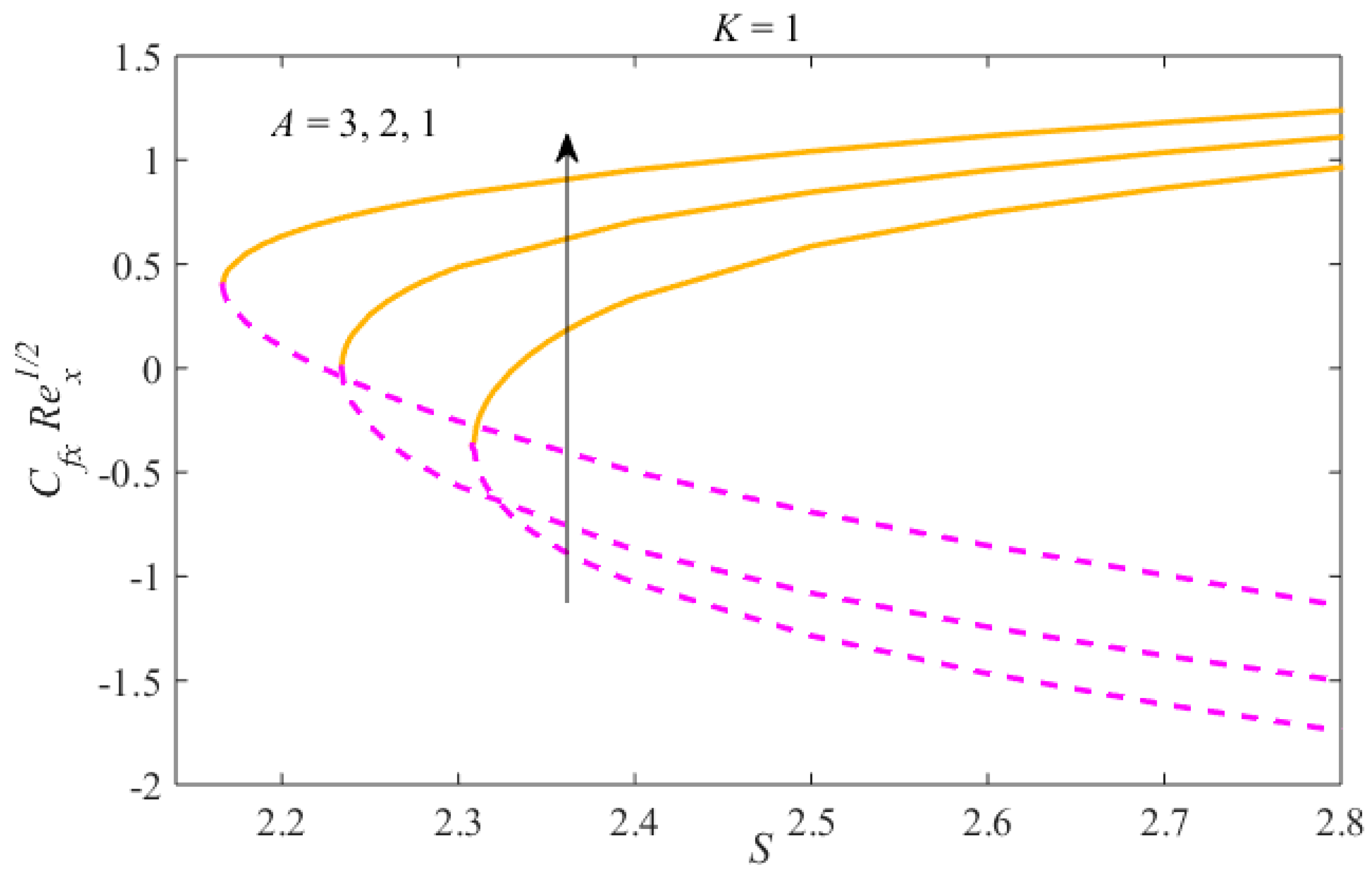
• Multiple results have been obtained for decelerating flow only, and for precise values of $S$.
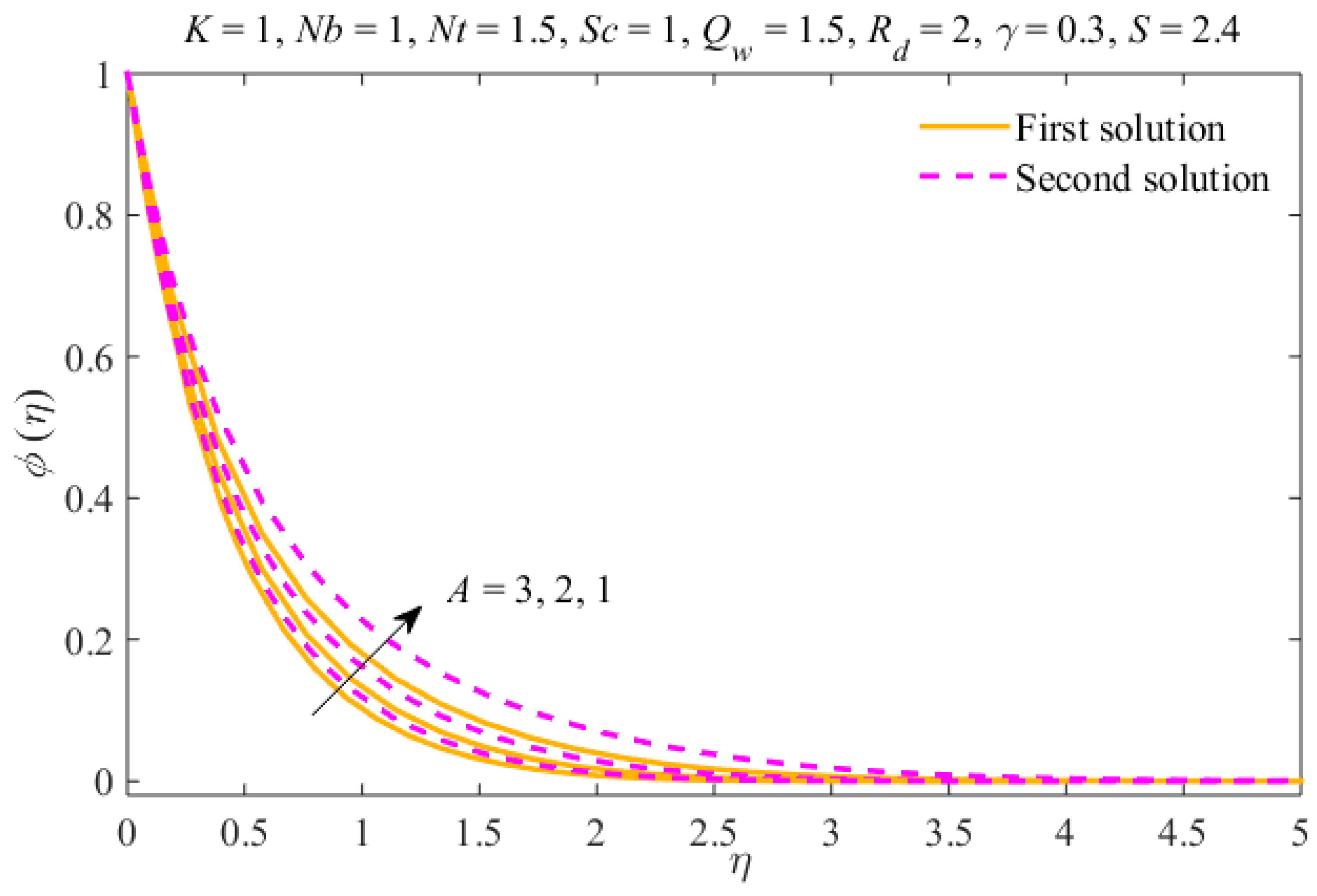
• The liquid velocity declines in the first result and increases in the second due to $K$. The concentration and temperature fields rise in the first result and diminish in the second result.
• The thicknesses of the concentration and thermal boundary layers increase due to $\gamma$ in both results.
• The liquid temperature and nanomaterial concentration decrease due to thermal radiation in both results.
• The nanoparticles distribution can be controlled through the mechanism of Brownian motion and the thermophoresis effect.
• The time-dependent and non-Newtonian parameters delay the separation of the boundary.

References

1. Keçebaş, A.; Yürüsoy, M. Similarity solutions of unsteady boundary layer equations of a special third grade fluid. Int. J. Eng. Sci. 2006, 44, 721–729. [Google Scholar] [CrossRef]
2. Ellahi, R.; Riaz, A. Analytical solutions for MHD flow in a third-grade fluid with variable viscosity. Math. Comput. Model. 2010, 52, 1783–1793. [Google Scholar] [CrossRef]
3. Sahoo, B.; Do, Y. Effects of slip on sheet-driven flow and heat transfer of a third grade fluid past a stretching sheet. Int. Comm. Heat Mass Transf. 2010, 37, 1064–1071. [Google Scholar] [CrossRef]
4. Sahoo, B.; Poncet, S. Flow and heat transfer of a third grade fluid past an exponentially stretching sheet with partial slip boundary condition. Int. J. Heat Mass Transf. 2011, 54, 5010–5019. [Google Scholar] [CrossRef] [Green Version]
5. Abbasbandy, S.; Hayat, T. On series solution for unsteady boundary layer equations in a special third grade fluid. Commun. Nonlinear Sci. Numer. Simul. 2011, 16, 3140–3146. [Google Scholar] [CrossRef]
6. Rehman, A.; Nadeem, S.; Malik, M.Y. Boundary layer stagnation-point flow of a third grade fluid over an exponentially stretching sheet. Braz. J. Chem. Eng. 2013, 30, 611–618. [Google Scholar] [CrossRef] [Green Version]
7. Hussain, T.; Hayat, T.; Shehzad, S.A.; Alsaedi, A.; Chen, B. A model of solar radiation and Joule heating in flow of third grade nanofluid. Z. Nat. A 2015, 70, 177–184. [Google Scholar] [CrossRef]
8. Naganthran, K.; Nazar, R.; Pop, I. Unsteady stagnation-point flow and heat transfer of a special third grade fluid past a permeable stretching/shrinking sheet. Sci. Rep. 2016, 6, 24632. [Google Scholar] [CrossRef] [Green Version]
9. Reddy, G.J.; Hiremath, A.; Kumar, M. Computational modeling of unsteady third-grade fluid flow over a vertical cylinder: A study of heat transfer visualization. Results Phys. 2018, 8, 671–682. [Google Scholar] [CrossRef]
10. Choi, S.U.S.; Eastman, J.A. Enhancing thermal conductivity of fluids with nanoparticles. In Proceedings of the 1995 International Mechanical Engineering Congress and Exhibition, San Francisco, CA, USA, 12–17 November 1995. [Google Scholar]
11. Masuda, H.; Ebata, A.; Teramae, K.; Hishinuma, N. Alteration of thermal conductivity and viscosity of liquid by dispersing ultra-fine particles. Netsu Bussei 1993, 7, 227–233. [Google Scholar] [CrossRef]
12. Buongiorno, J. Convective transport in nanofluids. ASME J. Heat Transf. 2006, 128, 240–250. [Google Scholar] [CrossRef]
13. Khan, W.A.; Pop, I. Boundary-layer flow of a nanofluid past a stretching sheet. Int. J. Heat Mass Transf. 2010, 53, 2477–2483. [Google Scholar] [CrossRef]
14. Rana, P.; Bhargava, R. Flow and heat transfer of a nanofluid over a nonlinearly stretching sheet: A numerical study. Commun. Nonlinear Sci. Numer. Simul. 2012, 17, 212–226. [Google Scholar] [CrossRef]
15. Makinde, O.D.; Aziz, A. Boundary layer flow of a nanofluid past a stretching sheet with a convective boundary condition. Int. J. Therm. Sci. 2011, 50, 1326–1332. [Google Scholar] [CrossRef]
16. Irfan, M.; Khan, M.; Khan, W.A.; Ayaz, M. Modern development on the features of magnetic field and heat sink/source in Maxwell nanofluid subject to convective heat transport. Phys. Lett. A 2018, 382, 1992–2002. [Google Scholar] [CrossRef]
17. Khan, M.; Irfan, M.; Khan, W.A. Impact of heat source/sink on radiative heat transfer to Maxwell nanofluid subject to revised mass flux condition. Results Phys. 2018, 9, 851–857. [Google Scholar] [CrossRef]
18. Zaib, A.; Abelman, S.; Chamkha, A.J.; Rashidi, M.M. Entropy generation in a Williamson nanofluid near a stagnation point over a moving plate with binary chemical reaction and activation energy. Heat Transf. Res. 2018, 49, 1131–1149. [Google Scholar] [CrossRef]
19. Bibi, M.; Rehman, K.-U.; Malik, M.Y.; Tahir, M. Numerical study of unsteady Williamson fluid flow and heat transfer in the presence of MHD through a permeable stretching surface. Eur. Phys. J. Plus 2018, 133, 154. [Google Scholar] [CrossRef]
20. Hayat, T.; Khan, S.A.; Khan, M.I.; Alsaedi, A. Theoretical investigation of Ree-Eyring nanofluid flow with entropy optimization and Arrhenius activation energy between two rotating disks. Comp. Methods Prog. Biomed. 2019, 177, 57–68. [Google Scholar] [CrossRef]
21. Aziz, A. A similarity solution for laminar thermal boundary layer over a flat plate with a convective surface boundary condition. Commun. Nonlinear Sci. Numer. Simul. 2009, 14, 1064–1068. [Google Scholar] [CrossRef]
22. Makinde, O.D.; Aziz, A. MHD mixed convection from a vertical plate embedded in a porous medium with a convective boundary condition. Int. J. Therm. Sci. 2010, 49, 1813–1820. [Google Scholar] [CrossRef]
23. Ishak, A. Similarity solutions for flow and heat transfer over a permeable surface with convective boundary condition. Appl. Math. Comput. 2014, 217, 837–842. [Google Scholar] [CrossRef]
24. Yao, S.; Fang, T.; Zhong, Y. Heat transfer of a generalized stretching/shrinking wall problem with convective boundary conditions. Commun. Nonlinear Sci. Numer. Simul. 2011, 16, 752–760. [Google Scholar] [CrossRef]
25. Rahman, M.M.; Merkin, J.H.; Pop, I. Mixed convection boundary-layer flow past a vertical flat plate with a convective boundary condition. Acta Mech. 2015, 226, 2441–2460. [Google Scholar] [CrossRef]
26. Mustafa, M.; Khan, J.A.; Hayat, T.; Alsaedi, A. Simulations for Maxwell fluid flow past a convectively heated exponentially stretching sheet with nanoparticles. AIP Adv. 2015, 5. [Google Scholar] [CrossRef] [Green Version]
27. Ibrahim, W.; Haq, R.U. Magnetohydrodynamic (MHD) stagnation point flow of nanofluid past a stretching sheet with convective boundary condition. J. Braz. Soc. Mech. Sci. Eng. 2016, 38, 1155–1164. [Google Scholar] [CrossRef]
28. Makinde, O.D.; Khan, W.A.; Khan, Z.H. Stagnation point flow of MHD chemically reacting nanofluid over a stretching convective surface with slip and radiative heat. Proc. Inst. Mech. Eng. Part E J. Process Mech. Eng. 2017, 231, 695–703. [Google Scholar] [CrossRef]
29. Khan, M.; Hashim; Hussain, M.; Azam, M. Magnetohydrodynamic flow of Carreau fluid over a convectively heated surface in the presence of non-linear radiation. J. Magn. Magn. Mater. 2016, 412, 63–68. [Google Scholar] [CrossRef]
30. Mabood, F.; Khan, W.A. Analytical study for unsteady nanofluid MHD flow impinging on heated stretching sheet. J. Mol. Liq. 2016, 219, 216–223. [Google Scholar] [CrossRef]
31. Fosdick, R.L.; Rajagopal, K.R. Thermodynamics and stability of fluids of third grade. Proc. R. Sot. Lond. A 1980, 339, 351. [Google Scholar] [CrossRef]
32. Mahapatra, T.R.; Nandy, S.K. Slip effects on unsteady stagnation-point flow and heat transfer over a shrinking sheet. Meccanica 2013, 48, 1599–1606. [Google Scholar] [CrossRef]
33. Ali, F.M.; Nazar, R.; Arifin, N.M.; Pop, I. Unsteady flow and heat transfer past an axisymmetric permeable shrinking sheet with radiation effect. Int. J. Numer. Meth. Fluids 2011, 67, 1310–1320. [Google Scholar] [CrossRef]
34. Rohni, A.M. Flow over an unsteady shrinking sheet with suction in a nanofluid. Int. Conf. Math. Comput. Biol. 2012, 9, 511–519. [Google Scholar] [CrossRef]
35. Merkin, J.H. On dual solutions occurring in mixed convection in a porous medium. J. Eng. Math. 1986, 20, 171–179. [Google Scholar] [CrossRef]
36. Weidman, P.D.; Kubitschek, D.G.; Davis, A.M.J. The effect of transpiration on self-similar boundary layer flow over moving surfaces. Int. J. Eng. Sci. 2006, 44, 730–737. [Google Scholar] [CrossRef]
37. Roşca, A.V.; Pop, I. Flow and heat transfer over a vertical permeable stretching/shrinking sheet with a second order slip. Int. J. Heat Mass Transf. 2013, 60, 355–364. [Google Scholar] [CrossRef]
38. Roşca, N.C.; Pop, I. Mixed convection stagnation point flow past a vertical flat plate with a second order slip: Heat flux case. Int. J. Heat Mass Transf. 2013, 65, 102–109. [Google Scholar] [CrossRef]
39. Ridha, A. Aiding flows non-unique similarity solutions of mixed-convection boundary-layer equations. Z. Angew. Math. Phys. 1996, 47, 341–352. [Google Scholar] [CrossRef]
Figure 1. The velocity profiles for different values of A .
Symmetry 12 00195 g001
Figure 2. The temperature profiles for different values of A .
Symmetry 12 00195 g002
Figure 3. The concentration profiles for different values of A .
Symmetry 12 00195 g003
Figure 4. The velocity profiles for different values of K .
Symmetry 12 00195 g004
Figure 5. The temperature profiles for different values of K .
Symmetry 12 00195 g005
Figure 6. The concentration profiles for different values of K .
Symmetry 12 00195 g006
Figure 7. The temperature profiles for different values of N b .
Symmetry 12 00195 g007
Figure 8. The concentration profiles for different values of N b .
Symmetry 12 00195 g008
Figure 9. The temperature profiles for different values of N t .
Symmetry 12 00195 g009
Figure 10. The concentration profiles for different values of N t .
Symmetry 12 00195 g010
Figure 11. The temperature profiles for different values of γ .
Symmetry 12 00195 g011
Figure 12. The concentration profiles for different values of γ .
Symmetry 12 00195 g012
Figure 13. The temperature profiles for different values of R d .
Symmetry 12 00195 g013
Figure 14. The concentration profiles for different values of R d .
Symmetry 12 00195 g014
Figure 15. The skin friction C f Re x 1 / 2 versus S for different values of A .
Symmetry 12 00195 g015
Figure 16. The Nusselt number N u x Re x 1 / 2 versus S for different values of A .
Symmetry 12 00195 g016
Figure 17. The Sherwood number S h x Re x 1 / 2 versus S for different values of A .
Symmetry 12 00195 g017
Figure 18. The skin friction C f Re x 1 / 2 versus A for different values of K .
Symmetry 12 00195 g018
Figure 19. The Nusselt number N u x Re x 1 / 2 versus A for different values of K .
Symmetry 12 00195 g019
Figure 20. The Sherwood number, S h x Re x 1 / 2 , versus A for different values of K .
Symmetry 12 00195 g020