A Mathematical Model for Transport in Poroelastic Materials with Variable Volume:Derivation, Lie Symmetry Analysis, and Examples

Abstract

Fluid and solute transport in poroelastic media is studied. Mathematical modeling of such transport is a complicated problem because of the volume change of the specimen due to swelling or shrinking and the transport processes are nonlinearly linked. The tensorial character of the variables adds also substantial complication in both theoretical and experimental investigations. The one-dimensional version of the theory is less complex and may serve as an approximation in some problems, and therefore, a one-dimensional (in space) model of fluid and solute transport through a poroelastic medium with variable volume is developed and analyzed. In order to obtain analytical results, the Lie symmetry method is applied. It is shown that the governing equations of the model admit a non-trivial Lie symmetry, which is used for construction of exact solutions. Some examples of the solutions are discussed in detail.

1. Introduction

The mathematical description of transport processes in biological tissue and artificial permselective membranes is crucial for understanding the physiology and pathology of biological systems and the effectiveness of artificial life supporting systems [1,2]. In particular, such problems involve transport through the biological tissue as in peritoneal dialysis, handling of transport through the pathological tissue as solid tumors, transport across polymer permselective membranes used in hemodialysis, or other membrane separation processes [1,2,3,4]. Another frequent application is the transport across soil and rock [5]. The investigated systems may involve transport across the permselective layer or penetration from one side to the impermeable layer on the other side. Transport of fluid and solutes is strongly related to the local properties of such a permselective membrane that might not be constant, but also altered by the transport processes itself [1,3,6,7,8]. In particular, the transport of fluid may result under some circumstances in the change of hydration of the material and subsequently in the change of its shape and volume. Such changes in the size of the specimen are typically not taken into account, and the theory is derived for a fixed size of the transport medium, even if the change of hydration is included the model [1,3,7,8]. Therefore, such models can be effective for small alterations in the meta-hydration only. The changes in the hydration of size of the specimen might affect the selective properties of the medium, and therefore, the understanding of the relation between hydration-related structural changes and membrane transport properties is crucial for the effectiveness of its application. Some examples of such systems are the tissue or artificial membrane exposed to an external fluid if the external hydrostatic and/or osmotic pressure is subject to changes [9,10] or the tissue if its internal fluid homeostasis is disturbed by changes in hydrostatic and/or osmotic pressure of blood and/or interstitial fluid [1,3,4,5,7,8,11].

It should be stressed that we consider elasticity and transport processes at the macroscale level. Of course, there are also many studies (see, e.g., [12,13,14,15,16]) devoted to the phenomena at the meso- and micro-scale (as a single protein channel in a cellular membrane [12], for example).

The first attempt to investigate transport processes through such a porous, elastic medium that might be deformed is to consider one-dimensional transport, i.e., along one axis or as in the case of spherical symmetry. An approach that is typically applied for the description of (bio)mechanical characteristics of the poroelastic material combined with its transport parameters is the theory of poroelasticity [5,11,12,13,14,15,16,17,18,19]. The theory in general involves higher order tensors, includes many parameters, and is difficult for mathematical, numerical, and experimental investigations [5,17,18,19]. The one-dimensional version (in space) of the theory is less complex and yields a simplified tensor structure. Nevertheless, the obtained model of the one-dimensional changes of the specimen caused by the alteration of membrane hydration (due to its swelling or shrinking) evokes the problem known as the “moving boundary”, which together with the nonlinearity of the theory and several variables involved, makes the task of finding the analytical solution very difficult.

We attempted to analyze a one-dimensional model of fluid and solute transport through a poroelastic medium with variable volume. Because the model in question is nonlinear and involves several nonlinear partial differential equations (PDEs), we do not expect its full integrability without essential simplifications. Thus, in order to obtain particular analytical results, we apply the Lie symmetry method [20,21,22], which is one of the most powerful methods to construct particular solutions of nonlinear PDEs at the present time.

The paper is organized as follows. In Section 2, the basic model for the poroelastic materials with the variable volume is developed in the 1D space approximation. In Section 3, the method of Lie symmetries is applied to the system of governing equations of the model. It is shown that this system admits a non-trivial Lie symmetry, and this allowed us to construct a variety of exact solutions. In Section 4, the solutions obtained are used to present some examples highlighting the volume change of poroelastic materials. Finally, we briefly discuss the result obtained in the last section.

2. Derivation of the Mathematical Model in 1D Approximation

The mathematical model for the poroelastic materials (PEM) with the variable volume is developed under the following assumptions:

• 1D approximation in space;
• no internal sources/sinks (however, they may be added);
• incompressible fluid;
• isothermal conditions for tissue transport.

The governing equations of the model consist of continuity equations.The first one expresses the volume balance for an infinitesimal volume element $dV$ of PEM as:

$$\frac{1}{dV}\frac{\partial dV}{\partial t}=\frac{\partial e}{\partial t}=\frac{\partial }{\partial t}\left(\frac{\partial u}{\partial x}\right)=-\frac{\partial }{\partial x}{\overline{j}}_V$$

(1)

where the deformation vector u is defined as:

$$u\left(x,t;X\right)=x\left(t\right)-X,X=x\left(0\right),$$

(2)

and the function $e=\frac{\partial u}{\partial x}$ is called dilatation, ${\overline{j}}_V$ the volumetric flux across the PEM, X the initial position within PEM, and $x\left(t\right)$ the position at time t, i.e., after displacement. For the derivation of this equation and subsequent to those, we used the theory described in [17,18,19]. It comes from continuity law for the mass $\rho dV$ of the infinitesimal element $dV$ and the mass density $\rho$ that:

$$\frac{1}{dV}\frac{\partial \left(\rho dV\right)}{\partial t}=\frac{\partial \rho }{\partial t}+\rho \frac{\partial e}{\partial t}=-\frac{\partial }{\partial x}{\overline{j}}_{\rho }$$

i.e.,

$$\frac{\partial \rho }{\partial t}=-\frac{\partial }{\partial x}{\overline{j}}_{\rho }+\rho \frac{\partial }{\partial x}{\overline{j}}_V,$$

(3)

where $j_{\rho }$ is the flux of mass with density $\rho$ through the PEM.

Let us consider PEM with two phases distinguished: the fluid phase, F, with the fractional volume ${\theta }_F$, and the solid phase, i.e., the matrix phase, M, with the fractional volume ${\theta }_M$, then the volume balance for each phase separately is:

$$\frac{1}{dV}\frac{\partial \left({\theta }_{F}dV\right)}{\partial t}=\frac{\partial {\theta }_F}{\partial t}+{\theta }_F\frac{\partial e}{\partial t}=-\frac{\partial }{\partial x}{\overline{j}}_{VF}$$

(4)

$$\frac{1}{dV}\frac{\partial \left({\theta }_{M}dV\right)}{\partial t}=\frac{\partial {\theta }_M}{\partial t}+{\theta }_M\frac{\partial e}{\partial t}=-\frac{\partial }{\partial x}{\overline{j}}_{VM}$$

(5)

so that:

$$\frac{\partial {\theta }_F}{\partial t}=-\frac{\partial }{\partial x}{\overline{j}}_{VF}+{\theta }_F\frac{\partial }{\partial x}{\overline{j}}_V$$

(6)

$$\frac{\partial {\theta }_M}{\partial t}=-\frac{\partial }{\partial x}{\overline{j}}_{VM}+{\theta }_M\frac{\partial }{\partial x}{\overline{j}}_V,$$

(7)

where ${\overline{j}}_{VF}$ and ${\overline{j}}_{VM}$ correspond to the volumetric fluxes in the fluid and matrix phases, respectively. Similarly for the densities, the equations:

$$\frac{1}{dV}\frac{\partial \left({\rho }_F{\theta }_{F}dV\right)}{\partial t}=\frac{\partial \left({\rho }_F{\theta }_F\right)}{\partial t}+{\rho }_F{\theta }_F\frac{\partial e}{\partial t}=-\frac{\partial }{\partial x}\left({\rho }_F{\overline{j}}_{VF}\right)$$

(8)

$$\frac{1}{dV}\frac{\partial \left({\rho }_M{\theta }_{M}dV\right)}{\partial t}=\frac{\partial \left({\rho }_M{\theta }_M\right)}{\partial t}+{\rho }_M{\theta }_M\frac{\partial e}{\partial t}=-\frac{\partial }{\partial x}\left({\rho }_M{\overline{j}}_{VM}\right)$$

(9)

take place, with densities ${\rho }_F$ and ${\rho }_M$ in the fluid and matrix phases, respectively. Note that the relation:

$$\rho ={\rho }_F{\theta }_F+{\rho }_M{\theta }_M$$

(10)

holds for the two phase PEM. Moreover, since the fluid is incompressible, ${\rho }_F$ is constant.

Since the solute with the concentration $c(t,x)$ is in fact dissolved in the fluid phase, we might write the corresponding equation for the volume balance:

$$\frac{1}{dV}\frac{\partial \left(c{\theta }_{F}dV\right)}{\partial t}=\frac{\partial \left(c{\theta }_F\right)}{\partial t}+c{\theta }_F\frac{\partial e}{\partial t}=-\frac{\partial }{\partial x}{\overline{j}}_S,$$

(11)

where ${\overline{j}}_S$ is the solute flux across the PEM. Finally, the dynamics of the PEM element of the mass $\rho dV$ with the velocity $\frac{\partial x}{\partial t}=\frac{\partial u}{\partial t}$ is described by the Newton law:

$$\frac{1}{dV}\frac{\partial \left(\rho \frac{\partial u}{\partial t}dV\right)}{\partial t}=\rho \frac{{\partial }^{2}u}{\partial t^2}+\frac{\partial u}{\partial t}\left(\frac{\partial \rho }{\partial t}+\rho \frac{\partial e}{\partial t}\right)=\frac{\partial }{\partial x}{\tilde{\tau }}_t$$

(12)

where ${\tilde{\tau }}_t$ is the Terzaghi effective stress tensor [23]. This tensor in the linear poroelastic theory for isotropic materials in 1D approximation is defined as:

$${\tilde{\tau }}_t=-\left(p-\sigma RTc\right)+(\lambda +2\mu )e,$$

i.e.,

$${\tilde{\tau }}_t=-\left(p-\sigma RTc\right)+(\lambda +2\mu )\frac{\partial u}{\partial x},$$

(13)

where $\lambda +2\mu$ is the elastic modulus with Lame constants $\lambda$ and $\mu$, and the effective pressure is given by the difference between hydrostatic pressure p and osmotic pressure $\sigma RTc$ with the reflection coefficient of PEM for the solute, $\sigma$, and constant $RT$ (gas constant times temperature). Note, that this tensor is also used in mathematical modeling of solid tumor growth [24,25].

Now, one needs to specify the fluxes across the PEM. In the fluid phase, we have:

$${\overline{j}}_{VF}={\overline{j}}_V^{rel}+{\theta }_F\frac{\partial u}{\partial t}$$

(14)

$${\overline{j}}_V^{rel}=-k\left(\frac{\partial p}{\partial x}-\sigma RT\frac{\partial c}{\partial x},\right)$$

(15)

where ${\overline{j}}_V^{rel}$ is the volumetric fluid flux relative to the matrix calculated according to the extended Darcy’s law with hydraulic conductivity k. Volumetric matrix flux is given by the equation:

$${\overline{j}}_{VM}={\theta }_M\frac{\partial u}{\partial t}$$

(16)

In contrast to the fluxes defined above, the solute flux through the PEM includes diffusive and convective terms as follows:

$${\overline{j}}_S={\overline{j}}_S^{rel}+{\theta }_{F}c\frac{\partial u}{\partial t},$$

(17)

and ${\overline{j}}_S^{rel}$ is the solute flux relative to the matrix defined as:

$${\overline{j}}_S^{rel}=-D\frac{\partial c_S}{\partial x}+Sc{\overline{j}}_{VF}^{rel},$$

(18)

where D stands for solute diffusivity in PEM and S is the sieving coefficient of the solute in the PEM. The fluxes arising in Equations (1) and (3) must be related to the above defined fluxes. Therefore, the relations:

$${\overline{j}}_V={\overline{j}}_{VF}+{\overline{j}}_{VM}=-k\left(\frac{\partial p}{\partial x}-\sigma RT\frac{\partial c}{\partial x}\right)+\frac{\partial u}{\partial t}$$

(19)

$${\overline{j}}_{\rho }={\rho }_F{\overline{j}}_{VF}+{\rho }_M{\overline{j}}_{VM}=-k\left(\frac{\partial p}{\partial x}-\sigma RT\frac{\partial c}{\partial x}\right){\rho }_F+\rho \frac{\partial u}{\partial t}$$

(20)

should take place.

Thus, Equations (6)–(9), (11) and (12) form a system of six partial differential equations for seven variables ${\theta }_F$, ${\theta }_M$, ${\rho }_F$, ${\rho }_M$, u, c and p; however, there is the known relation for the two phase PEM:

$${\theta }_F+{\theta }_M=1,$$

so that the number of governing equations is correct. Notably, Equation (1) is the sum of Equations (4) and (5) and therefore cannot be considered as independent from the other equations. Similarly, Equation (3) is a linear combination of Equations (8) and (9). Moreover, assuming that we are dealing with an incompressible fluid, we may set ${\rho }_F={\rho }_F^0=const$; therefore, Equation (8) can be skipped because one coincides with Equation (4).

All the notations arising in the above formulae are explained in

Table 1. Description of the symbols used in the formulae above.

Symbol	Description
$dV$	an infinitesimal volume element of PEM
u	deformation vector
e	dilatation
${\overline{j}}_V$	volumetric flow across PEM
$\rho$	mass density
$j_{\rho }$	mass flux across PEM
${\theta }_F$	fractional volume of fluid phase F
${\theta }_M$	fractional volume of matrix phase M
${\overline{j}}_{VF}$	fluid flux in phase F
${\overline{j}}_{VM}$	fluid flux in phase M
${\rho }_F$	mass density of fluid phase F
${\rho }_M$	mass density of matrix phase M
c	solute concentration in PEM
${\overline{j}}_S$	solute flux across the PEM
${\tilde{\tau }}_t$	Terzaghi effective stress tensor
p	mechanical pressure in PEM
$\sigma$	reflection coefficient of PEM
$RT$	gas constant times temperature
$\lambda +2\mu$	elastic modulus with Lame constants $\lambda$ and $\mu$
${\overline{j}}_V^{rel}$	volumetric flux relative to the matrix
${\overline{j}}_S^{rel}$	solute flux relative to the matrix
k	hydraulic conductivity
D	solute diffusivity in PEM
$S=1-\sigma$	sieving coefficient of solute in PEM

.

In order to write the governing equations in the explicit form, one needs to substitute the expressions for flows from (14)–(18) into Equations (6)–(9), and (11) and the Terzaghi effective stress tensor into (12). Taking into account the equalities (10) and ${\theta }_M=1-{\theta }_F$, we prefer to exclude the unknown functions ${\rho }_M$ and ${\theta }_M$ for the solid phase (matrix) in order to have a simpler equation corresponding to (1), instead of (7). Making the relevant calculations, we arrive at the nonlinear system consisting of five PDEs for unknown functions ${\theta }_F$, $\rho$, u, c, and p:

$$2u_{tx}=k(p_{xx}-{\sigma }_1{c}_{xx}),$$

(21)

$$\rho u_{tt}+{\rho }_t{u}_t+\rho u_t{u}_{tx}=(\lambda +2\mu )u_{xx}-(p_x-{\sigma }_1{c}_x),$$

(22)

$${\rho }_t+{\rho }_x{u}_t=k({\rho }_F^0-\rho )(p_{xx}-{\sigma }_1{c}_{xx}),$$

(23)

$${{\theta }_F}_t+{{\theta }_F}_x{u}_t=k\left(1-{\theta }_F\right)(p_{xx}-{\sigma }_1{c}_{xx}),$$

(24)

$${\left(c{\theta }_F\right)}_t+{\left(c{\theta }_F\right)}_x{u}_t+2c{\theta }_F{u}_{tx}=kS{\left(c(p_x-{\sigma }_1{c}_x)\right)}_x+D{c}_{xx},$$

(25)

where ${\sigma }_1=\sigma RT$ and ${\rho }_F={\rho }_F^0$ are positive constant and the lower subscripts t and x denote differentiation with respect to these variables.

In order to complete the mathematical model for PEM with variable volume, one needs to add the corresponding boundary conditions and initial profiles. Examples of such conditions are given in Section 3.

3. Lie Symmetry and Some Exact Solutions

Let us introduce the function that corresponds to the effective pressure:

$$p_x^{*}=p_x-{\sigma }_1{c}_x\equiv p_x-\sigma RT{c}_x$$

(26)

in order to simplify the PDE system (21)–(25). Then, the governing equations take the form:

$$\begin{array}{c}2u_{tx}=k{p}_{xx}^{*},\hfill \\ \rho u_{tt}+{\rho }_t{u}_t+\rho u_t{u}_{tx}={\lambda }^{*}{u}_{xx}-p_x^{*},\hfill \\ {\rho }_t+{\rho }_x{u}_t=k({\rho }_F^0-\rho )p_{xx}^{*},\hfill \\ {{\theta }_F}_t+{{\theta }_F}_x{u}_t=k\left(1-{\theta }_F\right)p_{xx}^{*},\hfill \\ {\left(c{\theta }_F\right)}_t+{\left(c{\theta }_F\right)}_x{u}_t+2c{\theta }_F{u}_{tx}=kS{\left(c{p}_x^{*}\right)}_x+D{c}_{xx},\hfill \end{array}$$

(27)

where $u(t,x),\rho (t,x),p^{*}(t,x),{\theta }_F(t,x)$, and $c(t,x)$ are unknown functions, while $k>0,{\lambda }^{*}=\lambda +2\mu >0,0\le S\le 1$, and $D\ge 0$ are some known constants.

Firstly, we find steady-state solutions of the system (27) using the well-known ansatz:

$$\begin{array}{c}u=u\left(x\right),\rho =\rho \left(x\right),p^{*}=p^{*}\left(x\right),{\theta }_F={\theta }_F\left(x\right),c=c\left(x\right).\hfill \end{array}$$

(28)

Substituting the ansatz (28) into system (27), one obtains the reduced system of ODEs:

$${\lambda }^{*}{u}^{″}-{p^{*}}^{\prime }=0,{p^{*}}^{″}=0,D{c}^{″}+kS{p^{*}}^{\prime }{c}^{\prime }=0.$$

(29)

(two equations in (27) simply vanish because ${p^{*}}^{″}=0$). The general solution of this system can be easily derived, and one has the form:

$$\begin{array}{c}u=a{x}^2+bx+u_0,\rho =\rho \left(x\right),p^{*}=p_0^{*}+2{\lambda }^{*}ax,{\theta }_F={\theta }_F\left(x\right),\hfill \\ c=\left\{\begin{array}{c}{c}_0+c_1{e}^{-\kappa x},\kappa =\frac{2{\lambda }^{*}akS}{D},SD\ne 0,\hfill \\ c_0+c_{1}x,S=0,D\ne 0,\hfill \\ c\left(x\right),S=D=0,\hfill \end{array}\right.\hfill \end{array}$$

(30)

where $a,b,u_0,p_0^{*},c_0$, and $c_1$ are arbitrary constants, while ${\theta }_F\left(x\right)$ and $\rho \left(x\right)$ are arbitrary smooth functions. Note that the subcase $S\ne 0,D=0$ leads to the constant pressure $p^{*}$ or/and concentration c what is rather inrealistic, hence one is skipped hereafter.

Now, we want to find the exact solutions of the system (27) with a more complicated mathematical structure with respect to the space and time variables. It should be stressed that the system (27) is essentially nonlinear (only the first equation is linear). At the present time, there is no existing general theory for the integration of nonlinear PDEs; hence, the construction of particular exact solutions for these equations remains an important mathematical problem. To the best of our knowledge, this problem was highlighted for the first time in the well-known book [26] (see also the discussion in the recent monograph [22]). Finding exact solutions that have a clear interpretation for the given process is of fundamental importance. Modern group-theoretical methods, which are based on the classical Lie method, are the most powerful methods to construct exact solutions of nonlinear PDEs. Here, we apply the Lie method, which is described in many excellent textbooks and monographs (see the most recent of those [20,21,22]). Therefore, applying Lie’s algorithm for finding Lie symmetries of the PDE system (27), we obtain the following statement.

Theorem 1.

System (27) with non-zero parameters $k,{\lambda }^{*},S$, and D is invariant under a infinity-dimensional Lie algebra generated by the Lie symmetries:

$${\partial }_t,{\partial }_x,{\partial }_u,x{\partial }_u,c{\partial }_c,g\left(t\right){\partial }_{p^{*}},$$

(31)

where $g\left(t\right)$ is an arbitrary smooth function (hereafter, the notations ${\partial }_z\equiv \frac{\partial }{\partial z},(z=t,x,u,c,p^{*})$ are used).

Proof of Theorem 1.

It is based on the infinitesimal criteria of invariance, which was formulated by S. Lie in h which was formulated by S. Lie in his pioneering works. In the case of a system of PDEs of arbitrary order, this criteria can be found, e.g., in [20] (see Section 1.2.5 therein). Note that the system (27) consists of five PDEs of the second order.

Therefore, a linear first-order operator of the form:

$$Y={\xi }_0{\partial }_t+{\xi }_1{\partial }_x+{\eta }_1{\partial }_u+{\eta }_2{\partial }_{\rho }+{\eta }_3{\partial }_{p^{*}}+{\eta }_4{\partial }_{{\theta }_F}+{\eta }_5{\partial }_c$$

(32)

(here, the coefficients ${\xi }_0,{\xi }_1$, and ${\eta }_i,i=1,\cdots ,5$ are to-be-determined functions of independent and dependent variables) is a Lie symmetry (operator of Lie’s invariance, point symmetry) of the system (27), provided the following five equalities take place:

$$\begin{array}{c}{Y}^{\left(2\right)}\left(2u_{tx}-k{p}_{xx}^{*}\right)=0,\hfill \\ Y^{\left(2\right)}\left(\rho u_{tt}+{\rho }_t{u}_t+\rho u_t{u}_{tx}-{\lambda }^{*}{u}_{xx}+p_x^{*}\right)=0,\hfill \\ Y^{\left(2\right)}\left({\rho }_t+{\rho }_x{u}_t-k({\rho }_F^0-\rho )p_{xx}^{*}\right)=0,\hfill \\ Y^{\left(2\right)}\left({{\theta }_F}_t+{{\theta }_F}_x{u}_t-k\left(1-{\theta }_F\right)p_{xx}^{*}\right)=0,\hfill \\ Y^{\left(2\right)}\left({\left(c{\theta }_F\right)}_t+{\left(c{\theta }_F\right)}_x{u}_t+2c{\theta }_F{u}_{tx}-kS{\left(c{p}_x^{*}\right)}_x-D{c}_{xx}\right)=0,\hfill \end{array}$$

(33)

for each solution $\left(u(t,x),\rho (t,x),p^{*}(t,x),{\theta }_F(t,x),c(t,x)\right)$ of the PDE system (27). Here, $Y^{\left(2\right)}$ is the second-order prolongation of the operator Y, which is again the linear first-order operator with coefficients defined by the well-known formulae via the first- and second-order derivatives of unknown coefficients ${\xi }_0,{\xi }_1$, and ${\eta }_i$ (see, e.g., [20], Section 1.2.1).

Substituting the expression for $Y^{\left(2\right)}$ into (33) and having done long calculations (see many examples in the books cited above), one arrives at a linear system of PDEs (the so-called system of determining equations) to find the functions ${\xi }_0,{\xi }_1$, and ${\eta }_i$. Because the system of determining equations is always linear and overdetermined (the number of PDEs is larger than that of unknown functions) and all the coefficients of the system (27) are some constants (no variable coefficients), the functions ${\xi }_0,{\xi }_1$, and ${\eta }_i$ can be derived by straightforward calculations. Moreover, one may use the computer algebra packages such as Maple and Mathematica for such purposes. We used Maple 18, and the result is presented in (31). □

Having such a wide Lie algebra of invariance (31), one has several possibilities to reduce the system (27) to systems of ODEs in order to find exact solutions with different structures. For example, using the Lie symmetry ${\partial }_t$, one immediately identifies the ansatz (28) leading to steady-state solutions.

Now, we are looking for exact solutions with more complicated structures. First of all, we remind the reader that any linear combination of Lie symmetry operators from (31) is also a Lie symmetry of (27) [20,21,22]. The most general combination involves all the operators (31) and reads as:

$$Y={\alpha }_0{\partial }_t+{\alpha }_1{\partial }_x+({\alpha }_2+{\alpha }_{3}x){\partial }_u+{\alpha }_{4}g\left(t\right){\partial }_{p^{*}}+{\alpha }_{5}c{\partial }_c$$

(34)

where ${\alpha }_i,i=0\cdots 5$ are arbitrary parameters.

The operator Y (34) contains six arbitrary parameters ${\alpha }_i,i=0\cdots 5$ and the function $g\left(t\right)$; hence, a non-trivial problem arises regarding how to classify inequivalent linear combinations of these operators leading to inequivalent exact solutions of the system (27). Solving this problem lies beyond this paper, but here, we consider some important particular cases, which allow finding non-trivial exact solutions of the system (27).

Let us take the following particular case of (34):

$$Y={\partial }_t+\alpha {\partial }_x+\beta x{\partial }_u+g\left(t\right){\partial }_{p^{*}}$$

where $\alpha ={\alpha }_1\ne 0$ and $\beta ={\alpha }_3$ are arbitrary, while other ${\alpha }_i$ are equal to zero or one. According to the standard procedure, we construct the so-called invariance surface conditions for unknown functions $u,p^{*},c,\rho$, and ${\theta }_F$ by acting the operator Y on these functions (see, e.g., pages 13–14 in [22] for details). For example, one easily obtains the equation:

$$u_t+\alpha u_x=\beta x$$

in the case of the function $u(t,x)$. Obviously, it is the linear first-order PDE with the general solution:

$$u=\frac{\beta x^2}{2\alpha }+f_1(x-\alpha t),$$

(35)

where $f_1$ is an arbitrary function. In the case of the pressure $p^{*}$, one arrives at the equation:

$$p_t^{*}+\alpha p_x^{*}=g\left(t\right),$$

which is also integrable and has the general solution:

$$p^{*}=p_0\left(t\right)+f_3(x-\alpha t),$$

(36)

where $f_3$ is again an arbitrary function, while $p_0\left(t\right)=\int g\left(t\right)dt$. Making analogous calculations for the function $c,\rho$, and ${\theta }_F$ and using (35) and (36), we obtain:

$$\begin{array}{c}u=\frac{\beta x^2}{2\alpha }+f_1\left(\omega \right),\rho =f_2\left(\omega \right),p^{*}=p_0\left(t\right)+f_3\left(\omega \right),\hfill \\ {\theta }_F=f_4\left(\omega \right),c=f_5\left(\omega \right),\hfill \end{array}$$

(37)

where $\omega =x-\alpha t$ and $f_i,i=1,\cdots ,6$ are arbitrary functions.

Now, we consider (37) as an ansatz (a special kind of substitution) for the system (27), which involves six unknown functions $f_i,i=1,\cdots ,6$.

Remark 1.

In the case $\beta =p_0\left(t\right)=0$, this ansatz reduces to the well-known substitution for finding plane wave solutions (in particular, traveling fronts).

Substituting the ansatz (37) into each equation of (27) and making the relevant calculations, we arrive at the ODE system:

$$\begin{array}{c}2\alpha f_1^{″}=-k{f}_3^{″},\hfill \\ {\left(f_2{f}_1^{\prime }\right)}^{\prime }+\frac{1}{2}{f}_2{\left({f_1^{\prime }}^2\right)}^{\prime }=\frac{{\lambda }^{*}\beta }{{\alpha }^3}+\frac{{\lambda }^{*}}{{\alpha }^2}{f}_1^{″}-\frac{f_3^{\prime }}{{\alpha }^2},\hfill \\ \left(1+f_1^{\prime }\right)f_2^{\prime }=-\frac{k\rho }{\alpha }{f}_3^{″}+\frac{k}{\alpha }{f}_2{f}_3^{″},\hfill \\ \left(1+f_1^{\prime }\right)f_4^{\prime }=\frac{k}{\alpha }\left(f_4-1\right)f_3^{″},\hfill \\ \left(1+f_1^{\prime }\right){\left(f_4{f}_5\right)}^{\prime }+2f_4{f}_5{f}_1^{″}=-\frac{1}{\alpha }\left(kS{\left(f_5{f}_3^{\prime }\right)}^{\prime }+D{f}_5^{″}\right),\hfill \end{array}$$

(38)

which is called the reduced system (for the system (27)).

Now, we obtain from the first and fourth equations of the system (38)”

$$f_3=-\frac{2\alpha }{k}{f}_1+{\gamma }_{31}\omega +{\gamma }_{30},f_4=1+\frac{{\gamma }_{41}}{{\left(1+f_1^{\prime }\right)}^2}$$

(39)

(hereafter, ${\gamma }_{ij}$ are arbitrary constants).

There is a special case $f_1^{\prime }=-1$, when the system (38) is integrable with the general solution:

$$\begin{array}{c}{f}_1=-\omega +{\gamma }_{10},f_2=\frac{1}{{\alpha }^3}\left(\alpha {\gamma }_{31}-{\lambda }^{*}\beta \right)\omega +{\gamma }_{20},\hfill \\ f_3={\gamma }_{31}\omega +{\gamma }_{30},f_4=f\left(\omega \right),\hfill \\ f_5=\left\{\begin{array}{c}{\gamma }_{50}+{\gamma }_{51}exp\left(-\frac{kS{\gamma }_{31}}{D}\omega \right),SD\ne 0,\hfill \\ {\gamma }_{50}+{\gamma }_{51}\omega ,S=0,D\ne 0,\hfill \\ f_5\left(\omega \right),S=D=0.\hfill \end{array}\right.\hfill \end{array}$$

(40)

Thus, substituting the functions from (40) into (37), we obtain the multiparameter family of exact solutions of the system (27) with $SD\ne 0$:

$$\begin{array}{c}u=\frac{\beta x^2}{2\alpha }-x+\alpha t+{\gamma }_{10},\hfill \\ \rho =\frac{1}{{\alpha }^3}\left(\alpha {\gamma }_{31}-{\lambda }^{*}\beta \right)(x-\alpha t)+{\gamma }_{20},\hfill \\ p^{*}=p_0\left(t\right)+{\gamma }_{31}(x-\alpha t)+{\gamma }_{30},\hfill \\ {\theta }_F=f(x-\alpha t),\hfill \\ c={\gamma }_{51}exp\left(-\frac{kS{\gamma }_{31}}{D}(x-\alpha t)\right)+{\gamma }_{50},\hfill \end{array}$$

(41)

Remark 2.

The parameters ${\gamma }_{10}$ and ${\gamma }_{30}$ can be skipped in the formulae (41) without losing generality.

Now, we return to the general case $f_1^{\prime }\ne -1$. Integrating the third equation of the system (38), we obtain:

$$f_2={\rho }_F^0+\frac{{\gamma }_{20}}{{\left(1+f_1^{\prime }\right)}^2}.$$

(42)

To complete the integrating of the system (38), one needs to solve the nonlinear second-order ODE:

$${\left(f_2{f}_1^{\prime }\right)}^{\prime }+\frac{1}{2}{f}_2{\left({f_1^{\prime }}^2\right)}^{\prime }=\frac{{\lambda }^{*}\beta }{{\alpha }^3}+\frac{{\lambda }^{*}}{{\alpha }^2}{f}_1^{″}-\frac{f_3^{\prime }}{{\alpha }^2},$$

(43)

i.e.,

$$-\frac{{\lambda }^{*}}{{\alpha }^2}{f}_1^{″}+{\left(\left({\rho }_F^0+\frac{{\gamma }_{20}}{{\left(1+f_1^{\prime }\right)}^2}\right)f_1^{\prime }\right)}^{\prime }+\frac{1}{2}\left({\rho }_F^0+\frac{{\gamma }_{20}}{{\left(1+f_1^{\prime }\right)}^2}\right){\left({f_1^{\prime }}^2\right)}^{\prime }=\frac{{\lambda }^{*}\beta }{{\alpha }^3}-\frac{{\gamma }_{31}}{{\alpha }^2}$$

(44)

with respect to the function $f_1$. The nonlinear ODE (43) is integrable; however, its general solution essentially depends on the parameters arising in the equation. In the most general case, its general solution cannot be identified explicitly. However, setting ${\gamma }_{20}=0$, we easily obtain:

$$f_1\left(\omega \right)=u_0+\frac{{\nu }_0-1}{{\nu }_0}\omega \pm \frac{1}{3\gamma {\nu }_0^2}{\left(2{\nu }_0\gamma ({\omega }_0-\omega )\right)}^{3/2}$$

(45)

if $\gamma =\frac{\beta }{\alpha }-\frac{{\gamma }_{31}}{{\lambda }^{*}}\ne 0$ and ${\nu }_0={\rho }_F^0\frac{{\alpha }^2}{{\lambda }^{*}}\ne 0$. Here, $u_0$ and ${\omega }_0$ are arbitrary constants. The special case $\gamma =0$ is examined below.

Finally, the linear second-order ODE:

$$\left(1+f_1^{\prime }\right){\left(f_4{f}_5\right)}^{\prime }+2f_4{f}_5{f}_1^{″}=-\frac{1}{\alpha }\left(kS{\left(f_5{f}_3^{\prime }\right)}^{\prime }+D{f}_5^{″}\right)$$

(46)

with respect to the function $f_5$, where the functions $f_3$ and $f_4$ have the form (39), should be solved. Because ODE (46) is an equation with variable coefficients (see (45)) and cannot be solved in terms of elementary functions, we consider here only a particular solution.

It can be noted that the linear function:

$$f_1={\nu }_1\omega +{\nu }_0,$$

(here, ${\nu }_1\ne 0$ and ${\nu }_0$ are arbitrary constants) is a particular solution of ODE (44) with ${\gamma }_{31}=\frac{{\lambda }^{*}\beta }{\alpha }$. In this case, ODE (46) can be solved; hence, we obtain

$$f_5=\left\{\begin{array}{c}{\gamma }_{50}+{\gamma }_{51}exp\left(-\frac{\kappa }{D\alpha }\omega \right),\kappa D\ne 0,\hfill \\ {\gamma }_{50}+{\gamma }_{51}\omega ,\kappa =0,D\ne 0,\hfill \\ f_5\left(\omega \right),\kappa =D=0,\hfill \end{array}\right.$$

(47)

where $\kappa =k{\lambda }^{*}\beta S+{\gamma }_{50}{\alpha }^2(1+{\nu }_1).$

Thus, substituting the functions $f_i,i=1,\dots ,5$ obtained above into the ansatz (37), we arrive at the exact solution:

$$\begin{array}{c}u=\frac{\beta x^2}{2\alpha }+{\nu }_1(x-\alpha t)+{\nu }_0,\hfill \\ \rho ={\gamma }_{20},\hfill \\ p^{*}=p_0\left(t\right)+\frac{{\lambda }^{*}\beta }{\alpha }(x-\alpha t)+{\gamma }_{30},\hfill \\ {\theta }_F={\gamma }_{40},\hfill \\ c={\gamma }_{51}exp\left(-\frac{\kappa }{D\alpha }(x-\alpha t)\right)+{\gamma }_{50},\hfill \end{array}$$

(48)

of the nonlinear system in question in the case of $\kappa D\ne 0$.

4. Some Examples and Their Interpretation

Here, we present non-trivial examples in order to show the applicability of the exact solutions obtained.

Let us consider the transport of fluid induced by mechanical and osmotic pressure with the given pressures at the surfaces: at $x=x_0$, mechanical pressure $p\left(x_0\right)=p_0$, and the concentration that induces osmotic pressure is $c\left(x_0\right)=c_0$. At $x=(L_S+x_0)$, let us assume that $p(L_S+x_0)=p_{ex}$ and concentration $c(L_S+x_0)=c_{ex}$. Let as denote by $p^{*}$ effective pressure acting at the PEM layer such that $p^{*}\left(x\right)=p\left(x\right)-\sigma RTc\left(x\right)$, $p^{*}\left(x_0\right)=p_0^{*}=p_0-\sigma RT{c}_0$, and $p^{*}\left(L_S\right)=p_{ex}^{*}=p_{ex}-\sigma RT{c}_{ex}$. Let us look for steady-state solutions. These solutions are found in Section 3 and presented in (29)).

Obviously, the steady-state solution (30) for u, $p^{*}$, and c can be rewritten as:

$$u\left(x\right)=\frac{a_1}{2{\lambda }^{*}}{(x-x_0)}^2+a_2\left(x-x_0\right)+u_0,$$

(49)

$$p^{*}\left(x\right)=a_1\left(x-x_0\right)+p_0^{*},$$

(50)

$$c\left(x\right)=c_0+a_3\left(exp\left[-\frac{kS{a}_1}{D}\left(x-x_0\right)\right]-1\right),$$

(51)

where $x_0$ is a reference point of the surface and $a_1$, $a_2$, and $a_3$ are some constants, and we assume that $DS\ne 0$.

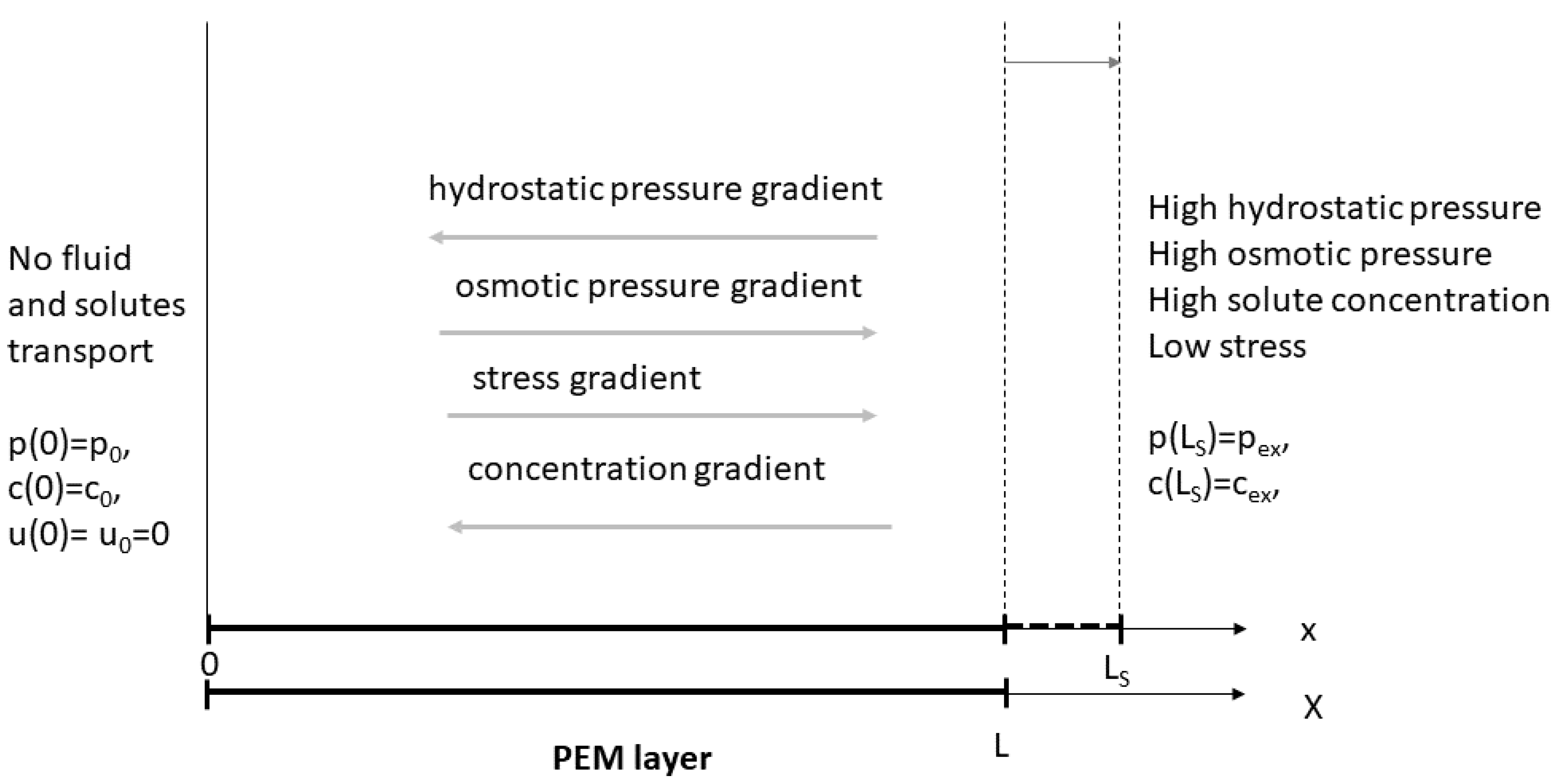
We may set $x_0=0$ without losing generality. Let us consider a layer of PEM in the steady-state with the surface at $x=0$ fixed in space and the other side at $x=L>0$ being in equilibrium with the same values of hydrostatic and osmotic pressures at both sides. Let us consider the steady-state obtained after a change of the pressure and concentration at one side of the PEM layer. This results in the deformation of the PEM layer and a displacement of its surfaces to a new positions $x=0$ and $x=L_S>0$ at the new steady-state. Let us assume that outside of both permeable boundaries, there are fluids with constant pressure and concentration. The exemplary arrangement of the forces considered in this example is presented in Figure 1 with X denoting the initial position in the PEM layer i.e., before displacement, and x denotes the position in PEM after displacement.

Therefore, in this case, the boundary conditions are as follows:

$$p\left(0\right)=p_0,p\left(L_S\right)=p_{ex},c\left(0\right)=c_0,c\left(L_S\right)=c_{ex},u\left(0\right)=u_0=0$$

We assume the following natural physical conditions:

(i) continuity of fluid pressure at both boundaries;

(ii) continuity of total stress across the free boundary at $x=L_S$; hence, the boundary condition (see Equation (13)) takes place:

$$-p_{ex}^{*}+{\lambda }^{*}\frac{\partial u}{\partial x}\left(L_s\right)=P,$$

(52)

where P is a given constant.

Obviously, Formula (50) and the boundary condition $p^{*}\left(L_S\right)=p_{ex}^{*}$ give:

$$a_1=\frac{\Delta p^{*}}{L_S},$$

(53)

where $\Delta p^{*}=p_{ex}^{*}-p_0^{*}=\Delta p-\sigma RT\Delta c$ and $\Delta p=p_{ex}-p_0,\Delta c=c_{ex}-c_0$ To find $a_2$, we use the boundary condition (52) and the above expression for $a_1$; thus:

$$a_2=-\frac{\Delta p^{*}}{{\lambda }^{*}}+\frac{P+p_{ex}^{*}}{{\lambda }^{*}}=\frac{P+p_0^{*}}{{\lambda }^{*}}.$$

(54)

Moreover, it comes from (51) and the boundary condition for $x=L_S$ that:

$$a_3=\frac{\Delta c}{exp\left[-\frac{kS\Delta p^{*}}{D}\right]-1},$$

(55)

To express the constant $L_S$ by the width of PEM L in the initial state when the pressure at both sides of the layer was equal to $p_0$, let us use Formula (49). Taking into account that the displacement $u=L_S-L$ (this follows from the definition of the displacement; see Formula (2)) and Formulas (53) and (54), we arrive at the expression:

$$L_S-L=\frac{1}{2L_S}\frac{\Delta p^{*}}{{\lambda }^{*}}{L_S}^2+\frac{P+p_0^{*}}{{\lambda }^{*}}{L}_S=\frac{P+p_{av}^{*}}{{\lambda }^{*}}{L}_S.$$

Thus, we find:

$$L_S=L/\left(1-\frac{P+p_{av}^{*}}{{\lambda }^{*}}\right),p_{av}^{*}=\frac{p_{ex}^{*}+p_0^{*}}{2}.$$

(56)

It should be noted that $L_S$ should be positive and within the range $L_{DRY}\le L_S<\infty$, where $L_{DRY}$ corresponds to a dry length of the PEM. Note, that if $P+p_{av}^{*}>0$, then $\frac{P+p_{av}^{*}}{{\lambda }^{*}}<1$, and therefore, $p_{av}^{*}<{\lambda }^{*}-P$. If $P+p_{av}^{*}\le 0$, we get that $1-\frac{P+p_{av}^{*}}{{\lambda }^{*}}<\frac{L}{L_{DRY}}$, which gives that $p_{av}^{*}>{\lambda }^{*}(1-\frac{L}{L_{DRY}})-P$. Therefore, the presented example in the case of a linear and constant stress tensor is valid for relatively small $p_{av}^{*}$ if compared to ${\lambda }^{*}$.

Finally, one may present the displacement as:

$$u\left(x\right)=\frac{\Delta p^{*}}{2L_S{\lambda }^{*}}{x}^2+\frac{P+p_0^{*}}{{\lambda }^{*}}x$$

(57)

the pressure as:

$$p^{*}\left(x\right)=\frac{\Delta p^{*}}{L_S}x+p_0^{*}.$$

(58)

and concentration as:

$$c\left(x\right)=c_0+a_3\left(exp\left[-\frac{kS\Delta p^{*}}{D{L}_S}x\right]-1\right),$$

(59)

with $L_S$ and $a_3$ given by (56) and (55), respectively, and $p\left(x\right)=p^{*}\left(x\right)+\sigma RTc\left(x\right)$. Note, that Formulas (57)–(59) are expressed as a function of x, which describes the position within the PEM layer after displacement. In order to express the above formulas as a function of initial position X, one has to substitute $u\left(x\right)=x-X$ into Equation (57). This would lead to the following expression:

$$x=\frac{-2(1-\sqrt{1+\alpha X})}{\alpha (1-\frac{p_0^{*}}{{\lambda }^{*}})},$$

(60)

where $\alpha =\frac{-2\Delta p^{*}({\lambda }^{*}-p_{av}^{*})}{L{({\lambda }^{*}-p_0^{*})}^2}$. Formulas for the functions $p^{*}\left(X\right)$ and $c\left(X\right)$ can be calculated by substituting (60) into formulae (58), (59), and $p\left(X\right)=p^{*}\left(X\right)+\sigma RTc\left(X\right)$.

Now, one may consider the further particular subcases.

(1) For example, set the boundary condition $P=p_{ex}^{*}$ as was used in [27]. Such a condition means that the total stress on the boundary surface is the same from both its sides, but in the opposite directions, and the fluid outside the material is at rest. Another option is to set $P=0$, which means that the poroelastic medium is fully relaxed, i.e., the effective stress disappears.

(2) If both boundaries can move freely and the pressure and concentration at both boundaries are equal to $p_{ex}$ and $c_{ex}$, then it is convenient to consider PEM of the initial width $2L$ and the middle point at $x=0$; this point is fixed in space by the symmetry of the problem, and there is no fluid flow across this surface. The steady-state of the system is described for each part of the membrane (to the left and right side of the middle point) separately by the above equations for $a_1=0$ and $a_3=0$, i.e., the effective pressure $p^{*}\left(x\right)=p_{ex}^{*}$ (as well as $p\left(x\right)=p_{ex}$ and $c\left(x\right)=c_{ex}$) is constant across PEM, and there is no flow across the tissue. Then, Formula (57) reduces to the form:

$$u\left(x\right)=\frac{P+p_{ex}^{*}}{{\lambda }^{*}}x$$

and the width of PEM compared to the width for $p_{ex}=0$ changes according to Formula (56) with $p_{av}^{*}=p_{ex}^{*}=p_0^{*}$.

(3) The boundary at $x=0$ is impermeable for the fluid. Then, the boundary condition at $x=0$ is $\frac{\partial p}{\partial x}=0$ and $\frac{\partial c}{\partial x}=0$, i.e., $a_1=0$ and $a_3=0$. Therefore, the effective pressure is again constant and equal to $p_{ex}^{*}$, and the dilatation u and the size of the tissue are described as above in (2).

In Figure 2, we present the profiles of the layer position, x, effective pressure, $p*$, solute concentration, c, and hydrostatic pressure, p, at the new steady-state as functions of the initial state position, X, for the two values of the elastic modulus that corresponds to the healthy tissue (interstitium) and the tumor tissue with ${\lambda }^{*}=100$ and ${\lambda }^{*}=700$, respectively, and $u\left(x\right)=x-X$. Let us assume that the initial steady-state was obtained for $p_0^{*}=0,c_0=0,p_0=0$, $p_{ex}^{*}=0,c_{ex}=0,p_{ex}=0$ and consider two cases that lead to the new steady-state: change in the hydrostatic pressure, i.e., $p_{ex}=30$, that results in $p_{ex}^{*}=30$ mmHg and a change in the osmotic pressure, caused by the increase of solute concentration $c_{ex}=30/\sigma /RT$ mmol/L, that results in $p_{ex}^{*}=-30$ mmHg.

5. Conclusions

In this paper, a mathematical model for the poroelastic materials (especially for biological tissue) with variable volume was developed under some assumptions. The model was built using the known conservation laws applied to poroelastic material, consisting of liquid and solid phases. As a result, a nonlinear system of governing equations was derived, which together with the relevant initial and boundary conditions formed the mathematical model.

The governing equations of the model were examined using the classical Lie method. It was shown that these equations admit a nontrivial Lie symmetry. Using the symmetries derived, some families of exact solutions, in particular steady-state (stationary) and plane wave solutions, were constructed.

Finally, steady-state solutions with correctly specified coefficients were studied in order to show that such solutions describe the volume change, i.e., displacement, in 1D space. Moreover, the relevant plots for some realistic data were constructed in order to show how the effective pressure $p^{*}$, hydrostatic pressure p, and the solute concentration, c, depend on the displacement, X.

Work is in progress to generalize the model on the case of higher dimensionality and to find exact solutions describing the volume change in time.

References

- Netti, P.A.; Baxter, L.T.; Boucher, Y.; Skalak, R.; Jain, R.K. Time dependent behavior of interstitial fluid in solid tumors: Implications for drug delivery. Cancer Res. 1995, 55, 5451–5458. [Google Scholar] [PubMed]
- Waniewski, J. Mathematical modeling of fluid and solute transport in hemodialysis and peritoneal dialysis. J. Membr. Sci. 2006, 274, 24–37. [Google Scholar] [CrossRef]
- Stachowska-Pietka, J.; Waniewski, J.; Flessner, M.F.; Lindholm, B. Distributed model of peritoneal fluid absorption. Am. J. Physiol. Heart Circ. Physiol. 2006, 291, H1862–H1874. [Google Scholar] [CrossRef]
- Cherniha, R.; Gozak, K.; Waniewski, J. Exact and Numerical Solutions of a Spatially-Distributed Mathematical Model for Fluid and Solute Transport in Peritoneal Dialysis. Symmetry 2016, 8, 50. [Google Scholar] [CrossRef] [Green Version]
- Detournay, E.; Cheng, A.H.-D. Fundamentals of poroelasticity in Comprehensive rock engineering: Principles, Practice and projects. In Analysis and Design Methods; Fairhust, C., Ed.; Pergamon Press: Oxford, UK, 1993; Volume II. [Google Scholar]
- Leiderman, R.; Barbone, P.E.; Oberai, A.A.; Bamber, J.C. Coupling between elastic strain and interstitial fluid flow: Ramifications for poroelastic imaging. Phys. Med. Biol. 2006, 51, 6291–6313. [Google Scholar] [CrossRef] [PubMed]
- Swartz, M.A.; Kaipainen, A.; Netti, P.A.; Brekken, C.; Boucher, Y.; Grodzinsky, A.J.; Jain, R.K. Mechanics of interstitial-lymphatic fluid transport: Theoretical foundation and experimental validation. J. Biomech. 1999, 32, 1297–1307. [Google Scholar] [CrossRef]
- Waniewski, J.; Stachowska-Pietka, J.; Flessner, M.F. Distributed modeling of osmotically driven fluid transport in peritoneal dialysis: Theoretical and computational investigations. Am. J. Physiol. Heart Circ. Physiol. 2009, 296, H1960–H1968. [Google Scholar] [CrossRef] [PubMed] [Green Version]
- Czyzewska, K.; Szary, B.; Waniewski, J. Transperitoneal transport of glucose in vitro. Artif. Organs 2000, 24, 857–863. [Google Scholar] [CrossRef] [PubMed]
- Galach, M.; Waniewski, J. Membrane transport of several ions during peritoneal dialysis: Mathematical modeling. Artif. Organs 2012, 36, E163–E178. [Google Scholar] [CrossRef] [PubMed]
- Li, P.; Schanz, M. Wave propagation in a 1-D partially saturated poroelastic column. Geophys. J. Int. 2011, 184, 1341–1353. [Google Scholar] [CrossRef] [Green Version]
- Gravelle, S.; Joly, L.; Detcheverry, F.; Ybert, C.; Cottin-Bizonne, C.; Bocquet, L. Optimizing water permeability through the hourglass shape of aquaporins. Proc. Natl. Acad. Sci. USA 2013, 110, 16367–16372. [Google Scholar] [CrossRef] [PubMed] [Green Version]
- Jain, R.K.; Tong, R.T.; Munn, L.L. Effect of Vascular Normalization by Antiangiogenic Therapy on Interstitial Hypertension, Peritumor Edema, and Lymphatic Metastasis: Insights from a Mathematical Model. Cancer Res. 2007, 67, 2729–2735. [Google Scholar] [CrossRef] [PubMed] [Green Version]
- Green, E.M.; Mansfield, J.C.; Bell, J.S.; Winlove, C.P. The structure and micromechanics of elastic tissue. Interface Focus 2014, 4, 20130058. [Google Scholar] [CrossRef] [PubMed] [Green Version]
- Wilson, W.; Van Donkelaar, C.C.; Van Rietbergen, B.; Huiskes, R. A fibril-reinforced poroviscoelastic swelling model for articular cartilage. J. Biomech. 2005, 38, 1195–1204. [Google Scholar] [CrossRef] [PubMed]
- Hänggi, P.; Marchesoni, F. Artificial Brownian motors: Controlling transport on the nanoscale. Rev. Mod. Phys. 2009, 81, 387. [Google Scholar] [CrossRef] [Green Version]
- Loret, B.; Simoes, F.M.F. Biomechanical Aspects of Soft Tissue; CRC Press: Boca Raton, FL, USA, 2017. [Google Scholar]
- Siddique, J.I.; Ahmed, A.; Aziz, A.; Khalique, C.M. A Review of Mixture Theory for Deformable Porous Media and Applications. Appl. Sci. 2017, 7, 917. [Google Scholar] [CrossRef] [Green Version]
- Taber, L.A. Nonlinear Theory of Elasticity. Applications in Biomechanics. 2004. Available online: https://www.worldscientific.com/worldscibooks/10.1142/5452 (accessed on 26 December 2019).
- Bluman, G.W.; Cheviakov, A.F.; Anco, S.C. Applications of Symmetry Methods to Partial Differential Equations; Springer: New York, NY, USA, 2010. [Google Scholar]
- Arrigo, D.J. Symmetry Analysis of Differential Equations; John Wiley & Sons: Hoboken, NJ, USA, 2015. [Google Scholar]
- Cherniha, R.; Serov, M.; Pliukhin, O. Nonlinear Reaction-Diffusion-Convection Equations: Lie and Conditional Symmetry, Exact Solutions and Their Applications; Chapman and Hall/CRC: New York, NY, USA, 2018. [Google Scholar]
- Terzaghi, K. Relation Between Soil Mechanics and Foundation Engineering: Presidential Address. In Proceedings of the First International Conference on Soil Mechanics and Foundation Engineering, Cambridge, MA, USA, 22–26 June 1936; Volume 3, pp. 13–18. [Google Scholar]
- Byrne, H.; King, J.R.; McElwain, D.L.S.; Preziosi, L. A two-phase model of solid tumour growth. Appl. Math. Lett. 2003, 16, 567–573. [Google Scholar] [CrossRef]
- Cherniha, R.; Davydovych, V. Lie symmetries, reduction and exact solutions of the (1+2)-dimensional nonlinear problem modeling the solid tumour growth. Commun. Nonlinear Sci. Numer. Simul. 2020, 80, 104980. [Google Scholar] [CrossRef]
- Ames, W.F. Nonlinear Partial Differential Equations in Engineering; Academic Press: New York, NY, USA, 1972. [Google Scholar]
- Netti, P.A.; Baxter, L.T.; Boucher, Y.; Skalak, R.; Jain, R.K. Macro- and microscopic fluid transport in living tissues: Application to solid tumors. Bioeng. Food Nat. Prod. 1997, 43, 818–834. [Google Scholar] [CrossRef]
Figure 1.
Exemplary arrangement of forces that are described in the model.A
Figure 2.
The profiles of the layer position, x, effective pressure, , solute concentration, c, and hydrostatic pressure, p, at the new steady-state as functions of the initial state position, X, for elastic modulus and and and mmHg.