Abstract
Our primary objective is to construct a plausible, unified model of inflation, dark energy and dark matter from a fundamental Lagrangian action first principle, wherein all fundamental ingredients are systematically dynamically generated starting from a very simple model of modified gravity interacting with a single scalar field employing the formalism of non-Riemannian spacetime volume-elements. The non-Riemannian volume element in the initial scalar field action leads to a hidden, nonlinear Noether symmetry which produces an energy-momentum tensor identified as the sum of a dynamically generated cosmological constant and dust-like dark matter. The non-Riemannian volume-element in the initial Einstein–Hilbert action upon passage to the physical Einstein-frame creates, dynamically, a second scalar field with a non-trivial inflationary potential and with an additional interaction with the dynamically generated dark matter. The resulting Einstein-frame action describes a fully dynamically generated inflationary model coupled to dark matter. Numerical results for observables such as the scalar power spectral index and the tensor-to-scalar ratio conform to the latest 2018 PLANCK data.
1. Introduction
In the last decade or so, a groundbreaking concept emerged regarding the intrinsic necessity to modify (extend) gravity theories beyond the framework of the norm—Einstein’s general relativity. The main motivation for these developments was to overcome the limitations of the latter coming from: (i) cosmology—for solving the problems of dark energy and dark matter and explaining the large scale structure of the Universe [1,2,3]; (ii) quantum field theory in curved spacetime—because of the non-renormalizabilty of ultraviolet divergences in higher loops [4,5,6,7,8,9]; (iii) modern string theory—because of the natural appearance of higher-order curvature invariants and scalar-tensor couplings in low-energy effective field theories [10,11,12,13,14].
Another parallel crucial development is the emergence of the theoretical framework based on the concept of "inflation," which is a necessary part of the standard model of cosmology, since it provides the solution to the fundamental puzzles of the old Big Bang theory, such as the horizon, the flatness and the monopole problems [15,16,17,18,19,20,21,22]. It can be achieved through various mechanisms; for instance, through the introduction of primordial scalar field(s) [23,24,25,26,27,28,29,30,31,32,33,34,35,36,37,38,39,40,41,42,43,44,45,46,47,48,49,50,51,52,53,54,55,56,57,58,59,60,61,62,63,64,65,66,67,68,69,70,71,72,73,74,75,76], or through correction terms into the modified gravitational action [77,78,79,80,81,82,83,84,85,86,87,88,89,90,91,92,93,94,95,96,97,98,99,100,101,102,103,104,105,106,107,108,109,110,111,112,113,114,115,116,117,118,119,120,121,122].
Additionally, inflation was proved crucial in providing a framework for the generation of primordial density perturbations [123,124]. Since these perturbations affect the cosmic background radiation (CMB), the inflationary effect on observations can be investigated through the prediction of the scalar spectral index of the curvature perturbations and its running, for the tensor spectral index and for the tensor-to-scalar ratio.
Various classes of modified gravity theories have been employed to construct viable inflationary models—-gravity; scalar-tensor gravity; Gauss–Bonnet gravity (see [125,126] for a detailed account)—and recently, models have been based on non-local gravity ([127] and references therein) or based on brane-world scenarios ([128] and references therein). The first successful cosmological model based on the extended -gravity produces the classical Starobinsky inflationary scalar field potential [16].
Dynamically generated models of inflation from modified/extended gravity such as the Starobinsky model [18,126,129,130] still remain viable and produce some of the best fits to existing observational data compared to other inflationary models [131].
Unification of inflation with dark energy and dark matter have been widely discussed [79,81,132,133,134,135,136,137,138,139,140,141,142]. It is indeed challenging to describe both phases of acceleration using a single scalar field minimally couple to gravity, without affecting the thermal history of the universe, which has been verified to a good degree of accuracy. In order to enable slow-roll behavior, the scalar field potential should exhibit shallow behavior early on, followed by a steep region for most of the universe’s history, and shallow behavior once again for later times. Although a simple exponential potential does not comply with the above picture, here we present a simple modified gravity model naturally providing a dynamically generated scalar potential, whose inflationary dynamics are compatible with the recent observational data. On the other hand, the task of describing particle creation will be discussed in our future work.
Another specific but broad class of modified (extended) gravitational theories is based on the formalism of non-Riemannian spacetime volume-elements. It was originally proposed in [143,144,145,146,147], and a subsequent, concise geometric formulation was proposed in in [148,149,150]. This formalism was used as a basis for constructing a series of extended gravity-matter models describing unified dark energy and dark matter scenarios [151,152]; quintessential cosmological models with gravity-assisted and inflaton-assisted dynamical suppression (in the "early" universe) or dynamical generation (in the post-inflationary universe) of electroweak spontaneous symmetry breaking and charge confinement [153,154]; and a novel mechanism for the dynamical supersymmetric Brout–Englert–Higgs effect in supergravity [148].
In the present paper our principal aim is to construct a plausible unified model, i.e., describing (most of the) principal physical manifestations of a unification of inflation and dark energy interacting with dark matter, where the formalism of the non-Riemannian spacetime volume-elements will play a fundamental role. To this end, we will consider a simple modified gravity interacting with a single scalar field where the Einstein–Hilbert part and the scalar field part of the action are constructed within the formalism of the non-Riemannian volume-elements—alternatives to the canonical Riemannian one . The non-Riemannian volume element in the initial scalar field action leads to a hidden, nonlinear Noether symmetry which produces an energy-momentum tensor identified as the sum of a dynamically generated cosmological constant and dynamically generated dust-like dark matter. The non-Riemannian volume-element in the initial Einstein–Hilbert action, upon passage to the physical Einstein-frame, creates, dynamically, a second scalar field with a non-trivial inflationary potential and with an additional interaction with the dynamically generated dark matter. The resulting Einstein-frame action describes a fully dynamically generated, unified model of inflation, dark energy and dark matter. Numerical results for observables such as the scalar power spectral index and the tensor-to-scalar ratio conform to the latest 2018 PLANCK data.
Let us briefly recall the essence of the non-Riemannian volume-form (volume-element) formalism. In integrals over differentiable manifolds (not necessarily a Riemannian one, so no metric is needed) volume-forms are given by non-singular maximal rank differential forms :
where
Our conventions for the alternating symbols and are: and ).
The volume element transforms as scalar density under general coordinate reparametizations.
In Riemannian D-dimensional spacetime manifolds, a standard, generally-covariant volume-form is defined through the "D-bein" (frame-bundle) canonical one-forms, ():
yields:
To construct modified gravitational theories as alternatives to ordinary standard theories in Einstein’s general relativity, instead of we can employ one or more alternative non-Riemannian volume element(s) as in (1) given by non-singular exact D-forms where:
so that the non-Riemannian volume element reads:
Thus, a non-Riemannian volume element is defined in terms of the (scalar density of the) dual field-strength of an auxiliary rank tensor gauge field .
The modified gravity Lagrangain actions based on the non-Riemannian volume-elements’ formalism are of the following generic form (here and in what follows we will use units with ):
where and are of the form (6) (for ), R is the scalar curvature, and the Lagrangian densities contain the matter fields (and possibly higher curvature terms; e.g., ).
A basic property of the class of actions (7) is that the equations of motion with respect to auxiliary gauge fields, defining the non-Riemannian volume-elements and as in (6), produce dynamically generated free integration constants , :
(cf. Equations (15) and (28) below) whose appearance will play an instrumental role in the sequel.
Further, let us stress the following important characteristic feature of the modified gravity-matter actions (7). When considering the gravity part in the first order (Palatini) framework (i.e., with a priori independent metric and affine connection ), then the auxiliary rank 3 tensor gauge fields defining the non-Riemannian volume-elements in (7) are almost pure-gauge degrees of freedom; i.e., they do not introduce any additional propagating gravitational degrees of freedom when passing to the physical Einstein-frame except for few discrete degrees of freedom with conserved canonical momenta appearing as arbitrary integration constants. This has been explicitly shown within the canonical Hamiltonian treatment [149,153].
On the other hand, when we treat (7) in the second order (metric) formalism (the affine connection is the canonical Levi–Civitta connection in terms of ), while passing to the physical Einstein-frame via conformal transformation (cf. Equation (30) below):
the first non-Riemannian volume element in (7) is not any more (almost) “pure gauge,” but creates a new dynamical canonical scalar field u via , which will play the role both of an inflaton field at early times, as well as driving late-time de Sitter expansion (see Section 3 below).
In Section 2 we briefly review our construction in [152] of a simple gravity-scalar-field model—a specific member of the class of modified gravitational models (7) of the form (10) below, which yields an explicit dynamical generation of independent (non-interacting among each other) dark energy and dark matter components in an unified description as a manifestation of a single material entity (“darkon” scalar field)— the simplest realization of a ΛCDM model.
In Section 3 we extend the previous construction to dynamically generate, apart from dark matter, early-time inflation and late-time de Sitter expansion as well—via dynamical creation of an additional canonical scalar field u (“inflaton”) out of a non-Riemannian volume-element with the following properties: (i) u acquires, dynamically, a non-trivial inflationary type scalar field potential driving inflation at early times of the universe’s evolution; (ii) At late times the same evolving u flows towards a stable critical point of the pertinent dynamical system describing the cosmological evolution, driving a late-time de Sitter expansion in a dark energy dominated epoch; (iii) In this case the field u induces a specific interaction between the dark energy and dark matter.
In Section 4 we study the cosmological implications of the latter dynamically generated inflationary model with interacting dark energy and dark matter. In Section 5 several plots of the numerical solutions for the evolution of the dynamical inflationary field and for the behavior of the relevant inflationary slow-roll parameters and the corresponding observables are presented. Section 6 contains our conclusions and outlook.
2. A Simple Model of Unification of Dark Energy and Dark Matter
In [152] we started with the following non-conventional gravity-scalar-field action—a simple particular case of the class (7)—containing one metric-independent non-Riemannian volume-element alongside with the standard Riemannian one:
with the following notations:
- The first term in (10) is the standard Einstein–Hilbert action with denoting the scalar curvature with respect to metric in the second order (metric) formalism;
- is particular representative of a non-Riemannian volume-element density (6):
- is general-coordinate invariant Lagrangian of a single scalar field :
Varying (10) with respect to , and yield the following equations of motion, respectively:
where is arbitrary integration constant (the factor 2 is for later convenience).
As stressed in [152], the scalar field dynamics are determined entirely by the first-order differential equation—the dynamical constraint Equation (15). The usual second order differential Equation (14) for is in fact a consequence of (15) together with the energy-momentum conservation:
Additionally, as exhibited in [152], the specific form of the scalar field potential does not affect the dynamics of the system (10); see the remark below following (18). The same phenomenon occurs in the extension of (10) to the model (24) in Section 3 and Section 4 below.
The canonical Hamiltonian analysis in [152] of the action (10) reveals that the auxiliary gauge field is in fact an almost pure-gauge; i.e., it is a non-propagating field-theoretic degree of freedom with the integration constant identified with the conserved Dirac-constrained canonical momentum conjugated to the “pure gauge,” “magnetic” component of . For a general canonical Hamiltonian treatment of Lagrangian action with one or more non-Riemannian volume-elements, we refer to [155].
A crucial property of the model (10) is the existence of a hidden nonlinear Noether symmetry revealed in [152]. Indeed, both Equations (14) and (15) can be equivalently rewritten in the following current-conservation law form:
The covariantly conserved current (17) is the Noether current corresponding to the invariance (modulo total derivative) of the action (10) with respect to the following hidden nonlinear symmetry transformations:
with — “dual” components of the auxiliary gauge field (11).
Remark 1.
The next important step is to rewrite (13) and (17) in the relativistic hydrodynamical form (again taking into account (15)):
Here the integration constant appears as a dynamically generated cosmological constant and:
We now find that the covariant conservation laws for the energy-momentum tensor (19) and the J-current (17) acquire the form:
Equations (21) imply in turn the geodesic equation for the “fluid” 4-velocity :
Therefore, comparing (19) with the standard expression for a perfect fluid stress-energy tensor , we see that (19) consists of two additive parts which have the following interpretations according to the standard Λ-CDM model [156,157,158,159,160,161,162,163] (using notations and ):
3. Inflation and Unified Dark Energy and Dark Matter
Now we will extend the simple model (10) of unified dark energy and dark matter by introducing another metric-independent non-Riemannian volume-element:
inside the gravity (Einstein–Hilbert) part of the action (using again units with ):
Here is a dimensionful parameter to be identified later on as energy scale of the inflationary universe’s epoch.
The specific form of the action (24) may be justified by the requirement of global Weyl-scale invariance under the transformations:
and provided we choose . Concerning globalWeyl-scale invariance, let us note that it played an important role already since the original papers on the non-canonical volume-form formalism [146]. In particular, models with spontaneously broken dilatation symmetry have been constructed along these lines, which are free of the fifth force problem [147].
The equations of motion of the action (24) with respect to and are the same as in (14) and (15); therefore, once again, (24) is invariant under the hidden, nonlinear Noether symmetry (18) with the associated Noether conserved current (17), which we rewrite here for later convenience, taking into account (15):
On the other hand, the equations of motion with respect to and now read:
where is the same energy-momentum tensor as in (13) or (19), which taking into account (15) and using short-hand notation in (26)) reads and is another free integration constant similar to in (15). Taking a trace of (27) together with (28) implies a dynamical equation for ( and as defined in (26) and (28), respectively):
The passage to the Einstein-frame is accomplished via the conformal transformation:
on Equations (27) and (29), and upon using the known formulae for conformal transformations of Ricci curvature tensor and covariant Dalambertian (see e.g., [164]; bars indicate magnitudes in the -frame):
In the process we introduce the field redefinition :
so that u appears as a canonical scalar field in the Einstein-frame transformed Equations (15), (27) and (29):
and most importantly, u acquires a non-trivial, dynamically degenerated potential:
due to the appearance of the free integration constants from the equations of motion of the original-frame, non-Riemannian spacetime volume-elements. The hidden, nonlinear Noether symmetry current conservation (17), equivalent to the -equation of motion, becomes in the Einstein-frame:
Thus, the Einstein-frame Lagrangian action producing the Einstein-frame equations of motion (34)–(38) reads:
with as in (37), in which (from (26)) becomes a simple Lagrange multiplier.
The upper line in (39) represents an inflationary Lagrangian action with dynamically generated inflationary potential (37) obtained in [107] from a pure gravity initial action (without any matter fields) in terms of non-Riemannian volume-elements:
which, as graphically depicted on Figure 1, is a generalization of the classic Starobinsky inflationary potential [16]. In fact, the latter is a special case of (37) for the particular values of the parameters: .
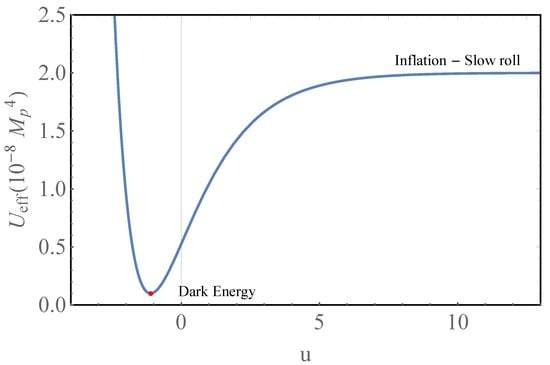
Figure 1.
Shape of the effective potential in the Einstein-frame (37). The physical unit for u is .
(37) possesses two main features relevant for cosmological applications:
- (ii) (37) has a stable minimum for a small finite value : for , where:
- (iii) As it will be explicitly exhibited in the dynamical system analysis in Section 4, the region of u around the stable minimum at (41) corresponds to the late-time de Sitter expansion of the universe with a slightly varied late-time Hubble parameter (dark energy dominated epoch), wherein the minimum value of the potential:is the asymptotic value at of the dynamical dark energy density [165,166].
The lower line in (39) represents the interaction between the dynamical inflaton field u and the “darkon” field ; in other words, here we have unification of inflation, dark energy and dark-matter. This is reflected in the structure of the Einstein-frame energy-momentum tensor (34)—the first two terms being the stress-energy tensor of u and the last term being the “darkon” stress-energy tensor coupled to u.
4. Cosmological Implications
Let us now consider reduction of the Einstein-frame action (39) to the Friedmann–Lemaitre–Robertson–Walker (FLRW) framework with metric , where and :
The equations of motion with respect to and from (43) are equivalent to the FLRW reduction of the dynamical constraint (36) and the Noether current conservation (38), respectively:
which imply the relation:
with a free integration constant. Taking into account (45), the FLRW reduction of the Einstein-frame energy-momentum tensor (34) becomes:
Relations (47) explicitly show that the last term in :
represents the “dust” dark matter part of the total energy denisty—it is “dust” because of absence ot corresponding contribution for the pressure p in (47).
The equation of motion from (43) with respect to u is ( being the Hubble parameter):
and finally, the two Friedmann equations (varying (43) with respect to lapse N and a) read:
Remark 2.
It is instructive to analyze the system FLRW Equations (49)–(51) as an autonomous dynamical system. To this end it is useful to rewrite the system (49)–(51) in terms of a set of dimensionless coordinates (following the approach in [167]):
with as in (42) and as in (48). In these coordinates the system defines a closed orbit:
which is equivalent to the first Friedmann Equation (50). Then, Equations (49) and (51) can be represented as a 3-dimensional autonomous dynamical system for the variables (cf. (52)):
where the primes indicate derivatives with respect to number of e-folds (meaning ).
The dynamical system (54)–(56) possesses two critical points:
- (A) Stable critical point:where all three eigenvalues of the stability matrix are negative or with negative real parts (). The stable critical point (57) corresponds to the late-time asymptotics of the universe’s evolution where according to the definitions (52) —the stable minimum of the effective potential (37), so that , the dark matter energy density (48) , and according to (56); i.e., late-time accelerated expansion with .
- (B) Unstable critical point:where one of the three eigenvalues of the stability matrix is zero (, , ). According to the definitions (52), in the vicinity of the unstable critical point (58), is very large positive (), so that , is vanishing and we have there a slow-roll inflationary evolution with inflationary scale where the standard slow-roll parameters are very small:
5. Numerical Solutions
Going back to the system of Equations (49)–(51), we can use (50) to replace the term in (49) and (51) so that we will obtain a closed system of two coupled nonlinear differential equations for of second and first order, respectively:
where is given by (37): .
Below we present several plots qualitatively illustrating the evolutionary behavior of the numerical solution of the system (61) and (62) with initial conditions conforming to the unstable critical point B (58): and —some large initial value. As a numerical example, for the purpose of graphical illustration, we will take the following numerical values of the parameters (the physical units would be ):
according to (42) (in reality is much smaller than 1/500 part of : [168,169] and ; cf. [170]).
On Figure 2 below, the plot represents the overall evolution of , whereas on Figure 3 are the plots for the slow-roll parameters and clearly indicating the end of inflation where their sharp grow-up starts.
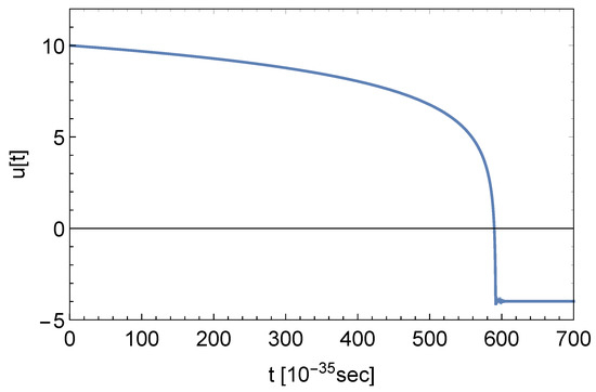
Figure 2.
Numerical shape of the evolution of . The physical unit for u is .
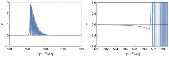
Figure 3.
Slow-roll parameters and before and around end of inflation. When the inflation ends.
Figure 4 represents the plot of the evolution of the Hubble parameter with a clear indication of the two (quasi-)de Sitter epochs—during early-times inflation with much higher value of , and in late-times with much smaller value of .
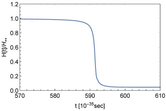
Figure 4.
Numerical shape of the evolution of . Here as in (58).
The plots on Figure 5 depict the oscillations of and occurring after the end of inflation.

Figure 5.
In the left panel—blown-up portion of the plot on Figure 2 around and after end of inflation depicting the oscillations of after end of inflation. In the right panel—oscillations of after end of inflation.
Figure 6 contains the plots of the evolution of —the parameter of the equation of state with a clear indication of a short time epoch of matter domination after end of inflation.
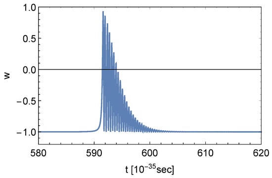
Figure 6.
Evolution of w parameter of the equation of state with sharp growth above for a short time interval after end of inflation—matter domination.
To obtain plausible values for the observables—the scalar power spectral index and the tensor to scalar ratio r [53,105,171]—we need the functional dependence of the slow-roll parameters and with respect to , the number of e-folds. More specifically, in is the number of e-folds at the end of inflation defined as ; then, we need the values and at —e-folds at the start of inflation, where it is assumed that . Then, according to [53,105]:
where the corresponding slow roll parameter reads:
and where is the functional dependence of Hubble parameter with respect to the number of e-folds. To this end we employ numerical simulation of the autonomous dynamical system Equations (54)–(56).
From the inflationary scenario, we know that the observed value of the inflationary scale is far larger than the current value (∼) of the cosmological constant (42). Thus, as in the numerical example above for the numerical solution of the system for (61) and (62), we will take again the values for the parameters according to (63), meaning that we set the initial condition for the Hubble parameter to be according to (58) . With those numerical values, we find the observables (64) to be:
which are well inside the last PLANCK observed constraints [131]:
In order to see the pattern of the general behavior depending on the initial conditions, we employ here Monte Carlo simulation with samples for the initial conditions using a normal distribution: , , while the error bar is taken to be .
Figure 7 shows how different values of initial conditions yield different numbers of e-folds until end of inflation (where ), and accordingly, different values for the observables r and , whereas Figure 8 depicts the corresponding relation between r and . Nevertheless, all the values of the latter fall within the constraint (67).
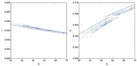
Figure 7.
The scalar to tensor ratio r and the scalar spectral index vs. the number of e-folds for different values of the initial conditions. The sampling of the latter is done with a normal distribution , .
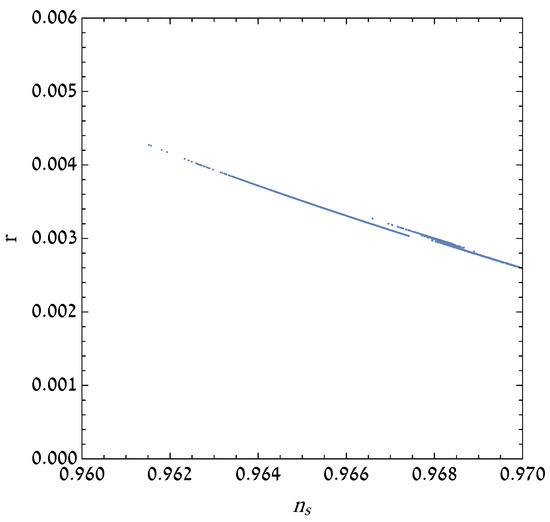
Figure 8.
The relation between the scalar to tensor ratio r and the scalar spectral index via sampled initial conditions with a normal distribution , . All of the sampled values fall well inside the Planck data constraint (67).
6. Conclusions and Outlook
In the present paper, starting from the basic first principle of Lagrangian field-theoretic actions combined with a non-canonical modification of gravity via employing non-Riemannian spacetime volume forms as alternatives to the standard Riemannian one given by , we have constructed a unified model of dynamically generated inflation with dark energy and dark matter coupled among themselves. Upon passage to the physical Einstein frame, our model captures the main properties of the slow-roll inflationary epoch in early times, the short period of matter domination after the end of inflation and the late-time epoch of de Sitter expansion—all driven by a dynamically created scalar inflaton field. The numerical results for the observables (scalar power spectral index and tensor to scalar ratio) conform to the 2018 PLANCK constraints.
In the present model, dark matter in the form of a dust-like fluid is created already in the early universe’s inflationary epoch without a significant impact on the inflationary dynamics. After the end of inflation, the dust-like dark matter, apart from a short period of matter domination, still does not exert a sufficient impact, which means that one has to further extend the present formulation in order to properly take the full dark matter contribution to the evolution into account.
One subject that has to be addressed is the “reheating of the universe,” since of course we need temperature in the early universe to account for processes such as Bing Bang nucleosynthesis. There are many ways to achieve this, due to the oscillating nature of inflaton solutions near the minimum of the inflaton potential, which leads in general to particle creation. For example, one possible way to complement the modified gravity-scalar field model (24) in order to incorporate the effect of radiation after end of inflation is to include a coupling to the “topological” density of a electromagnetic field with field strength in the following way:
Upon passage to the Einstein-frame via the conformal transformation (30), the action (68) becomes (cf. (39)):
The coupling term is suppressed in the inflationary stage where the derivative of u is small (because of the slow roll regime), whereas after end of inflation it may produce pairs of photons out of u due to the appreciable time-derivative of u resulting from the oscillations near the minimum of the effective potential. Of course, many other possible interaction terms can be introduced.
Finally, in the reheating stage, many particles can be produced; some of them could be no standard-model particles. If those are stable, they could provide additional “dark matter” apart from the “darkon” dust-like dark matter discussed here. Of course, if all created particles beyond those of the standard models turn out to be unstable, then we will be left with the “darkon” as the unique source of dark matter.
Author Contributions
All authors contributed equally to this work. All authors have read and agreed to the published version of the manuscript.
Funding
This research received no external funding.
Acknowledgments
We gratefully acknowledge support of our collaboration through the Exchange Agreement between Ben-Gurion University, Beer-Sheva, Israel, and Bulgarian Academy of Sciences, Sofia, Bulgaria. E.N. and S.P. are thankful for support of Contract DN 18/1 from the Bulgarian National Science Fund. D.B., E.G. and E.N. are also partially supported by COST Actions CA15117, CA16104 and CA18108.
Conflicts of Interest
The authors declare no conflict of interest.
References
- Perlmutter, S.; Aldering, G.; Goldhaber, G.; Knop, R.A.; Nugent, P.; Castro, P.G.; Deustua, S.; Fabbro, S.; Goobar, A.; Groom, D.E.; et al. Measurements of Omega and Lambda from 42 high redshift supernovae. Astrophys. J. 1999, 517, 565–586. [Google Scholar] [CrossRef]
- Copeland, E.J.; Sami, M.; Tsujikawa, S. Dynamics of dark energy. Int. J. Mod. Phys. 2006, D15, 1753–1936. [Google Scholar] [CrossRef]
- Novikov, E.A. Quantum Modification of General Relativity. Electron. J. Theor. Phys. 2016, 13, 79–90. [Google Scholar]
- Benitez, F.; Gambini, R.; Lehner, L.; Liebling, S.; Pullin, J. Critical collapse of a scalar field in semiclassical loop quantum gravity. Phys. Rev. Lett. 2020, 124, 071301. [Google Scholar] [CrossRef]
- Budge, L.; Campbell, J.M.; De Laurentis, G.; Keith Ellis, R.; Seth, S. The one-loop amplitude for Higgs + 4 gluons with full mass effects. arXiv 2020, arXiv:2002.04018. [Google Scholar]
- Bell, G.; Beneke, M.; Huber, T.; Li, X.Q. Two-loop non-leptonic penguin amplitude in QCD factorization. arXiv 2020, arXiv:2002.03262. [Google Scholar]
- Fröhlich, J.; Knowles, A.; Schlein, B.; Sohinger, V. A path-integral analysis of interacting Bose gases and loop gases. arXiv 2020, arXiv:2001.11714. [Google Scholar]
- D’Ambrosio, F. Semi-Classical Holomorphic Transition Amplitudes in Covariant Loop Quantum Gravity. arXiv 2020, arXiv:2001.04651. [Google Scholar]
- Novikov, E.A. Ultralight gravitons with tiny electric dipole moment are seeping from the vacuum. Mod. Phys. Lett. 2016, A31, 1650092. [Google Scholar] [CrossRef]
- Dekens, W.; Stoffer, P. Low-energy effective field theory below the electroweak scale: Matching at one loop. JHEP 2019, 10, 197. [Google Scholar] [CrossRef]
- Ma, C.T.; Pezzella, F. Stringy Effects at Low-Energy Limit and Double Field Theory. arXiv 2019, arXiv:1909.00411. [Google Scholar]
- Jenkins, E.E.; Manohar, A.V.; Stoffer, P. Low-Energy Effective Field Theory below the Electroweak Scale: Operators and Matching. JHEP 2018, 3, 16. [Google Scholar] [CrossRef]
- Brandyshev, P.E. Cosmological solutions in low-energy effective field theory for type IIA superstrings. Grav. Cosmol. 2017, 23, 15–19. [Google Scholar] [CrossRef]
- Gomez, C.; Jimenez, R. Cosmology from Quantum Information. arXiv 2020, arXiv:2002.04294. [Google Scholar]
- Guth, A.H. The Inflationary Universe: A Possible Solution to the Horizon and Flatness Problems. Phys. Rev. 1981, D23, 347–356. [Google Scholar] [CrossRef]
- Starobinsky, A.A. Spectrum of relict gravitational radiation and the early state of the universe. JETP Lett. 1979, 30, 682–685. [Google Scholar]
- Kazanas, D. Dynamics of the Universe and Spontaneous Symmetry Breaking. Astrophys. J. 1980, 241, L59–L63. [Google Scholar] [CrossRef]
- Starobinsky, A.A. A New Type of Isotropic Cosmological Models Without Singularity. Phys. Lett. 1980, 91B, 99–102. [Google Scholar] [CrossRef]
- Linde, A.D. A New Inflationary Universe Scenario: A Possible Solution of the Horizon, Flatness, Homogeneity, Isotropy and Primordial Monopole Problems. Phys. Lett. 1982, 108B, 389–393. [Google Scholar] [CrossRef]
- Albrecht, A.; Steinhardt, P.J. Cosmology for Grand Unified Theories with Radiatively Induced Symmetry Breaking. Phys. Rev. Lett. 1982, 48, 1220–1223. [Google Scholar] [CrossRef]
- Barrow, J.D.; Ottewill, A.C. The Stability of General Relativistic Cosmological Theory. J. Phys. 1983, A16, 2757. [Google Scholar] [CrossRef]
- Blau, S.K.; Guendelman, E.I.; Guth, A.H. The Dynamics of False Vacuum Bubbles. Phys. Rev. 1987, D35, 1747. [Google Scholar] [CrossRef]
- Cervantes-Cota, J.L.; Dehnen, H. Induced gravity inflation in the standard model of particle physics. Nucl. Phys. 1995, B442, 391–412. [Google Scholar] [CrossRef]
- Berera, A. Warm inflation. Phys. Rev. Lett. 1995, 75, 3218–3221. [Google Scholar] [CrossRef] [PubMed]
- Armendariz-Picon, C.; Damour, T.; Mukhanov, V.F. k - inflation. Phys. Lett. 1999, B458, 209–218. [Google Scholar] [CrossRef]
- Kanti, P.; Olive, K.A. Assisted chaotic inflation in higher dimensional theories. Phys. Lett. 1999, B464, 192–198. [Google Scholar] [CrossRef][Green Version]
- Garriga, J.; Mukhanov, V.F. Perturbations in k-inflation. Phys. Lett. 1999, B458, 219–225. [Google Scholar] [CrossRef]
- Gordon, C.; Wands, D.; Bassett, B.A.; Maartens, R. Adiabatic and entropy perturbations from inflation. Phys. Rev. 2000, D63, 023506. [Google Scholar] [CrossRef]
- Bassett, B.A.; Tsujikawa, S.; Wands, D. Inflation dynamics and reheating. Rev. Mod. Phys. 2006, 78, 537–589. [Google Scholar] [CrossRef]
- Chen, X.; Wang, Y. Quasi-Single Field Inflation and Non-Gaussianities. JCAP 2010, 1004, 27. [Google Scholar] [CrossRef]
- Germani, C.; Kehagias, A. New Model of Inflation with Non-minimal Derivative Coupling of Standard Model Higgs Boson to Gravity. Phys. Rev. Lett. 2010, 105, 011302. [Google Scholar] [CrossRef] [PubMed]
- Kobayashi, T.; Yamaguchi, M.; Yokoyama, J. G-inflation: Inflation driven by the Galileon field. Phys. Rev. Lett. 2010, 105, 231302. [Google Scholar] [CrossRef]
- Feng, C.J.; Li, X.Z.; Saridakis, E.N. Preventing eternality in phantom inflation. Phys. Rev. 2010, D82, 023526. [Google Scholar] [CrossRef]
- Burrage, C.; de Rham, C.; Seery, D.; Tolley, A.J. Galileon inflation. JCAP 2011, 1101, 14. [Google Scholar] [CrossRef]
- Kobayashi, T.; Yamaguchi, M.; Yokoyama, J. Generalized G-inflation: Inflation with the most general second-order field equations. Prog. Theor. Phys. 2011, 126, 511–529. [Google Scholar] [CrossRef]
- Ohashi, J.; Tsujikawa, S. Potential-driven Galileon inflation. JCAP 2012, 1210, 35. [Google Scholar] [CrossRef]
- Paliathanasis, A.; Tsamparlis, M. Two scalar field cosmology: Conservation laws and exact solutions. Phys. Rev. 2014, D90, 043529. [Google Scholar] [CrossRef]
- Dimakis, N.; Paliathanasis, A. Crossing the phantom divide line as an effect of quantum transitions. arXiv 2020, arXiv:2001.09687. [Google Scholar]
- Dimakis, N.; Paliathanasis, A.; Terzis, P.A.; Christodoulakis, T. Cosmological Solutions in Multiscalar Field Theory. Eur. Phys. J. 2019, C79, 618. [Google Scholar] [CrossRef]
- Benisty, D.; Guendelman, E.I. A transition between bouncing hyper-inflation to ΛCDM from diffusive scalar fields. Int. J. Mod. Phys. 2018, A33, 1850119. [Google Scholar] [CrossRef]
- Barrow, J.D.; Paliathanasis, A. Observational Constraints on New Exact Inflationary Scalar-field Solutions. Phys. Rev. 2016, D94, 083518. [Google Scholar] [CrossRef]
- Barrow, J.D.; Paliathanasis, A. Reconstructions of the dark-energy equation of state and the inflationary potential. Gen. Rel. Grav. 2018, 50, 82. [Google Scholar] [CrossRef] [PubMed]
- Olive, K.A. Inflation. Phys. Rept. 1990, 190, 307–403. [Google Scholar] [CrossRef]
- Linde, A.D. Hybrid inflation. Phys. Rev. 1994, D49, 748–754. [Google Scholar] [CrossRef] [PubMed]
- Liddle, A.R.; Parsons, P.; Barrow, J.D. Formalizing the slow roll approximation in inflation. Phys. Rev. 1994, D50, 7222–7232. [Google Scholar] [CrossRef] [PubMed]
- Lidsey, J.E.; Liddle, A.R.; Kolb, E.W.; Copeland, E.J.; Barreiro, T.; Abney, M. Reconstructing the inflation potential: An overview. Rev. Mod. Phys. 1997, 69, 373–410. [Google Scholar] [CrossRef]
- Hossain, M.W.; Myrzakulov, R.; Sami, M.; Saridakis, E.N. Variable gravity: A suitable framework for quintessential inflation. Phys. Rev. 2014, D90, 023512. [Google Scholar] [CrossRef]
- Wali Hossain, M.; Myrzakulov, R.; Sami, M.; Saridakis, E.N. Unification of inflation and dark energy à la quintessential inflation. Int. J. Mod. Phys. 2015, D24, 1530014. [Google Scholar] [CrossRef]
- Cai, Y.F.; Gong, J.O.; Pi, S.; Saridakis, E.N.; Wu, S.Y. On the possibility of blue tensor spectrum within single field inflation. Nucl. Phys. 2015, B900, 517–532. [Google Scholar] [CrossRef]
- Geng, C.Q.; Hossain, M.W.; Myrzakulov, R.; Sami, M.; Saridakis, E.N. Quintessential inflation with canonical and noncanonical scalar fields and Planck 2015 results. Phys. Rev. 2015, D92, 023522. [Google Scholar] [CrossRef]
- Kamali, V.; Basilakos, S.; Mehrabi, A. Tachyon warm-intermediate inflation in the light of Planck data. Eur. Phys. J. 2016, C76, 525. [Google Scholar] [CrossRef]
- Geng, C.Q.; Lee, C.C.; Sami, M.; Saridakis, E.N.; Starobinsky, A.A. Observational constraints on successful model of quintessential Inflation. JCAP 2017, 1706, 11. [Google Scholar] [CrossRef]
- Dalianis, I.; Kehagias, A.; Tringas, G. Primordial black holes from α-attractors. JCAP 2019, 1901, 37. [Google Scholar] [CrossRef]
- Dalianis, I.; Tringas, G. Primordial black hole remnants as dark matter produced in thermal, matter, and runaway-quintessence postinflationary scenarios. Phys. Rev. 2019, D100, 083512. [Google Scholar] [CrossRef]
- Benisty, D. Inflation from Fermions. arXiv 2019, arXiv:1912.11124. [Google Scholar]
- Benisty, D.; Guendelman, E.I. Inflation compactification from dynamical spacetime. Phys. Rev. 2018, D98, 043522. [Google Scholar] [CrossRef]
- Benisty, D.; Guendelman, E.I.; Saridakis, E.N. The Scale Factor Potential Approach to Inflation. arXiv 2019, arXiv:1909.01982. [Google Scholar]
- Gerbino, M.; Freese, K.; Vagnozzi, S.; Lattanzi, M.; Mena, O.; Giusarma, E.; Ho, S. Impact of neutrino properties on the estimation of inflationary parameters from current and future observations. Phys. Rev. 2017, D95, 043512. [Google Scholar] [CrossRef]
- Giovannini, M. Planckian hypersurfaces, inflation and bounces. arXiv 2020, arXiv:2001.11799. [Google Scholar]
- Brahma, S.; Brandenberger, R.; Yeom, D.H. Swampland, Trans-Planckian Censorship and Fine-Tuning Problem for Inflation: Tunnelling Wavefunction to the Rescue. arXiv 2020, arXiv:2002.02941. [Google Scholar]
- Domcke, V.; Guidetti, V.; Welling, Y.; Westphal, A. Resonant backreaction in axion inflation. arXiv 2020, arXiv:2002.02952. [Google Scholar]
- Tenkanen, T.; Tomberg, E. Initial conditions for plateau inflation. arXiv 2020, arXiv:2002.02420. [Google Scholar]
- Martin, J.; Papanikolaou, T.; Pinol, L.; Vennin, V. Metric preheating and radiative decay in single-field inflation. arXiv 2020, arXiv:2002.01820. [Google Scholar]
- Cheon, K.; Lee, J. N = 2 PNGB Quintessence Dark Energy. arXiv 2020, arXiv:2002.01756. [Google Scholar]
- Saleem, R.; Zubair, M. Inflationary solution of Hamilton Jacobi equations during weak dissipative regime. Phys. Scr. 2020, 95, 035214. [Google Scholar] [CrossRef]
- Giacintucci, S.; Markevitch, M.; Johnston-Hollitt, M.; Wik, D.R.; Wang, Q.H.S.; Clarke, T.E. Discovery of a giant radio fossil in the Ophiuchus galaxy cluster. arXiv 2020, arXiv:2002.01291. [Google Scholar] [CrossRef]
- Aalsma, L.; Shiu, G. Chaos and complementarity in de Sitter space. arXiv 2020, arXiv:2002.01326. [Google Scholar]
- Kogut, A.; Fixsen, D.J. Calibration Method and Uncertainty for the Primordial Inflation Explorer (PIXIE). arXiv 2020, arXiv:2002.00976. [Google Scholar]
- Arciniega, G.; Jaime, L.; Piccinelli, G. Inflationary predictions of Geometric Inflation. arXiv 2020, arXiv:2001.11094. [Google Scholar]
- Rasheed, M.A.; Golanbari, T.; Sayar, K.; Akhtari, L.; Sheikhahmadi, H.; Mohammadi, A.; Saaidi, K. Warm Tachyon Inflation and Swampland Criteria. arXiv 2020, arXiv:2001.10042. [Google Scholar]
- Aldabergenov, Y.; Aoki, S.; Ketov, S.V. Minimal Starobinsky supergravity coupled to dilaton-axion superfield. arXiv 2020, arXiv:2001.09574. [Google Scholar]
- Tenkanen, T. Tracing the high energy theory of gravity: an introduction to Palatini inflation. arXiv 2020, arXiv:2001.10135. [Google Scholar]
- Shaposhnikov, M.; Shkerin, A.; Zell, S. Standard Model Meets Gravity: Electroweak Symmetry Breaking and Inflation. arXiv 2020, arXiv:2001.09088. [Google Scholar]
- Garcia, M.A.G.; Amin, M.A.; Green, D. Curvature Perturbations From Stochastic Particle Production During Inflation. arXiv 2020, arXiv:2001.09158. [Google Scholar]
- Hirano, K. Inflation with very small tensor-to-scalar ratio. arXiv 2019, arXiv:1912.12515. [Google Scholar]
- Gialamas, I.D.; Lahanas, A.B. Reheating in R2 Palatini inflationary models. arXiv 2019, arXiv:1911.11513. [Google Scholar]
- Kawasaki, M.; Yamaguchi, M.; Yanagida, T. Natural chaotic inflation in supergravity. Phys. Rev. Lett. 2000, 85, 3572–3575. [Google Scholar] [CrossRef]
- Bojowald, M. Inflation from quantum geometry. Phys. Rev. Lett. 2002, 89, 261301. [Google Scholar] [CrossRef]
- Nojiri, S.; Odintsov, S.D. Modified gravity with negative and positive powers of the curvature: Unification of the inflation and of the cosmic acceleration. Phys. Rev. 2003, D68, 123512. [Google Scholar] [CrossRef]
- Kachru, S.; Kallosh, R.; Linde, A.D.; Maldacena, J.M.; McAllister, L.P.; Trivedi, S.P. Towards inflation in string theory. JCAP 2003, 310, 13. [Google Scholar] [CrossRef]
- Nojiri, S.; Odintsov, S.D. Unifying phantom inflation with late-time acceleration: Scalar phantom-non-phantom transition model and generalized holographic dark energy. Gen. Rel. Grav. 2006, 38, 1285–1304. [Google Scholar] [CrossRef]
- Ferraro, R.; Fiorini, F. Modified teleparallel gravity: Inflation without inflation. Phys. Rev. 2007, D75, 084031. [Google Scholar] [CrossRef]
- Cognola, G.; Elizalde, E.; Nojiri, S.; Odintsov, S.D.; Sebastiani, L.; Zerbini, S. A Class of viable modified f(R) gravities describing inflation and the onset of accelerated expansion. Phys. Rev. 2008, D77, 046009. [Google Scholar] [CrossRef]
- Cai, Y.F.; Saridakis, E.N. Inflation in Entropic Cosmology: Primordial Perturbations and non-Gaussianities. Phys. Lett. 2011, B697, 280–287. [Google Scholar] [CrossRef]
- Ashtekar, A.; Sloan, D. Probability of Inflation in Loop Quantum Cosmology. Gen. Rel. Grav. 2011, 43, 3619–3655. [Google Scholar] [CrossRef]
- Qiu, T.; Saridakis, E.N. Entropic Force Scenarios and Eternal Inflation. Phys. Rev. 2012, D85, 043504. [Google Scholar] [CrossRef]
- Briscese, F.; Marcianò, A.; Modesto, L.; Saridakis, E.N. Inflation in (Super-)renormalizable Gravity. Phys. Rev. 2013, D87, 083507. [Google Scholar] [CrossRef]
- Ellis, J.; Nanopoulos, D.V.; Olive, K.A. No-Scale Supergravity Realization of the Starobinsky Model of Inflation. Phys. Rev. Lett. 2013, 111, 111301. [Google Scholar] [CrossRef]
- Basilakos, S.; Lima, J.A.S.; Sola, J. From inflation to dark energy through a dynamical Lambda: An attempt at alleviating fundamental cosmic puzzles. Int. J. Mod. Phys. 2013, D22, 1342008. [Google Scholar] [CrossRef]
- Sebastiani, L.; Cognola, G.; Myrzakulov, R.; Odintsov, S.D.; Zerbini, S. Nearly Starobinsky inflation from modified gravity. Phys. Rev. 2014, D89, 023518. [Google Scholar] [CrossRef]
- Baumann, D.; McAllister, L. Inflation and String Theory; Cambridge Monographs on Mathematical Physics; Cambridge University Press: Cambridge, UK, 2015. [Google Scholar] [CrossRef]
- Dalianis, I.; Farakos, F. On the initial conditions for inflation with plateau potentials: the R+R2 (super)gravity case. JCAP 2015, 1507, 44. [Google Scholar] [CrossRef][Green Version]
- Kanti, P.; Gannouji, R.; Dadhich, N. Gauss-Bonnet Inflation. Phys. Rev. 2015, D92, 041302. [Google Scholar] [CrossRef]
- De Laurentis, M.; Paolella, M.; Capozziello, S. Cosmological inflation in F(R,) gravity. Phys. Rev. 2015, D91, 083531. [Google Scholar] [CrossRef]
- Basilakos, S.; Mavromatos, N.E.; Solà, J. Starobinsky-like inflation and running vacuum in the context of Supergravity. Universe 2016, 2, 14. [Google Scholar] [CrossRef]
- Bonanno, A.; Platania, A. Asymptotically safe inflation from quadratic gravity. Phys. Lett. 2015, B750, 638–642. [Google Scholar] [CrossRef]
- Koshelev, A.S.; Modesto, L.; Rachwal, L.; Starobinsky, A.A. Occurrence of exact R2 inflation in non-local UV-complete gravity. JHEP 2016, 11, 67. [Google Scholar] [CrossRef]
- Bamba, K.; Odintsov, S.D.; Saridakis, E.N. Inflationary cosmology in unimodular F(T) gravity. Mod. Phys. Lett. 2017, A32, 1750114. [Google Scholar] [CrossRef]
- Motohashi, H.; Starobinsky, A.A. f(R) constant-roll inflation. Eur. Phys. J. 2017, C77, 538. [Google Scholar] [CrossRef]
- Oikonomou, V.K. Autonomous dynamical system approach for inflationary Gauss–Bonnet modified gravity. Int. J. Mod. Phys. 2018, D27, 1850059. [Google Scholar] [CrossRef]
- Benisty, D.; Vasak, D.; Guendelman, E.; Struckmeier, J. Energy transfer from spacetime into matter and a bouncing inflation from covariant canonical gauge theory of gravity. Mod. Phys. Lett. 2019, A34, 1950164. [Google Scholar] [CrossRef]
- Benisty, D.; Guendelman, E.I. Two scalar fields inflation from scale-invariant gravity with modified measure. Class. Quant. Grav. 2019, 36, 095001. [Google Scholar] [CrossRef]
- Antoniadis, I.; Karam, A.; Lykkas, A.; Tamvakis, K. Palatini inflation in models with an R2 term. JCAP 2018, 1811, 28. [Google Scholar] [CrossRef]
- Karam, A.; Pappas, T.; Tamvakis, K. Frame-dependence of inflationary observables in scalar-tensor gravity. PoS 2019, CORFU2018, 64. [Google Scholar] [CrossRef]
- Nojiri, S.; Odintsov, S.D.; Saridakis, E.N. Holographic inflation. Phys. Lett. 2019, B797, 134829. [Google Scholar] [CrossRef]
- Benisty, D.; Guendelman, E.I.; Saridakis, E.N.; Stoecker, H.; Struckmeier, J.; Vasak, D. Inflation from fermions with curvature-dependent mass. arXiv 2019, arXiv:1905.03731. [Google Scholar] [CrossRef]
- Benisty, D.; Guendelman, E.; Nissimov, E.; Pacheva, S. Dynamically Generated Inflation from Non-Riemannian Volume Forms. arXiv 2019, arXiv:1906.06691. [Google Scholar] [CrossRef]
- Benisty, D.; Guendelman, E.I.; Nissimov, E.; Pacheva, S. Dynamically generated inflationary two-field potential via non-Riemannian volume forms. arXiv 2019, arXiv:1907.07625. [Google Scholar] [CrossRef]
- Kinney, W.H.; Vagnozzi, S.; Visinelli, L. The zoo plot meets the swampland: Mutual (in)consistency of single-field inflation, string conjectures, and cosmological data. Class. Quant. Grav. 2019, 36, 117001. [Google Scholar] [CrossRef]
- Brustein, R.; Sherf, Y. Causality Violations in Lovelock Theories. Phys. Rev. 2018, D97, 084019. [Google Scholar] [CrossRef]
- Sherf, Y. Hyperbolicity Constraints in Extended Gravity Theories. Phys. Scr. 2019, 94, 085005. [Google Scholar] [CrossRef]
- Capozziello, S.; De Laurentis, M.; Luongo, O. Connecting early and late universe by f(R) gravity. Int. J. Mod. Phys. 2014, D24, 1541002. [Google Scholar] [CrossRef]
- Gorbunov, D.; Tokareva, A. Scale-invariance as the origin of dark radiation? Phys. Lett. 2014, B739, 50–55. [Google Scholar] [CrossRef]
- Myrzakulov, R.; Odintsov, S.; Sebastiani, L. Inflationary universe from higher-derivative quantum gravity. Phys. Rev. 2015, D91, 083529. [Google Scholar] [CrossRef]
- Bamba, K.; Myrzakulov, R.; Odintsov, S.D.; Sebastiani, L. Trace-anomaly driven inflation in modified gravity and the BICEP2 result. Phys. Rev. 2014, D90, 043505. [Google Scholar] [CrossRef]
- Benisty, D.; Guendelman, E.I.; Vasak, D.; Struckmeier, J.; Stoecker, H. Quadratic curvature theories formulated as Covariant Canonical Gauge theories of Gravity. Phys. Rev. 2018, D98, 106021. [Google Scholar] [CrossRef]
- Aashish, S.; Panda, S. Covariant quantum corrections to a scalar field model inspired by nonminimal natural inflation. arXiv 2020, arXiv:2001.07350. [Google Scholar]
- Rashidi, N.; Nozari, K. Gauss-Bonnet Inflation after Planck2018. arXiv 2020, arXiv:2001.07012. [Google Scholar] [CrossRef]
- Odintsov, S.D.; Oikonomou, V.K. Geometric Inflation and Dark Energy with Axion F(R) Gravity. Phys. Rev. 2020, D101, 044009. [Google Scholar] [CrossRef]
- Antoniadis, I.; Karam, A.; Lykkas, A.; Pappas, T.; Tamvakis, K. Single-field inflation in models with an R2 term. In Proceedings of the 19th Hellenic School and Workshops on Elementary Particle Physics and Gravity (CORFU2019), Corfu, Greece, 31 August–25 September 2019. [Google Scholar]
- Benisty, D.; Guendelman, E.I. Correspondence between the first and second order formalism by a metricity constraint. Phys. Rev. 2018, D98, 044023. [Google Scholar] [CrossRef]
- Chakraborty, S.; Paul, T.; SenGupta, S. Inflation driven by Einstein-Gauss-Bonnet gravity. Phys. Rev. 2018, D98, 083539. [Google Scholar] [CrossRef]
- Mukhanov, V.F.; Chibisov, G.V. Quantum Fluctuations and a Nonsingular Universe. JETP Lett. 1981, 33, 532–535. [Google Scholar]
- Guth, A.H.; Pi, S.Y. Fluctuations in the New Inflationary Universe. Phys. Rev. Lett. 1982, 49, 1110–1113. [Google Scholar] [CrossRef]
- Faraoni, V.; Capozziello, S. Beyond Einstein Gravity; Springer: Dordrecht, The Netherlands, 2011; Volume 170. [Google Scholar] [CrossRef]
- Nojiri, S.; Odintsov, S.D.; Oikonomou, V.K. Modified Gravity Theories on a Nutshell: Inflation, Bounce and Late-time Evolution. Phys. Rept. 2017, 692, 1–104. [Google Scholar] [CrossRef]
- Dimitrijevic, I.; Dragovich, B.; Koshelev, A.S.; Rakic, Z.; Stankovic, J. Cosmological Solutions of a Nonlocal Square Root Gravity. Phys. Lett. 2019, B797, 134848. [Google Scholar] [CrossRef]
- Bilic, N.; Dimitrijevic, D.D.; Djordjevic, G.S.; Milosevic, M.; Stojanovic, M. Tachyon inflation in the holographic braneworld. JCAP 2019, 1908, 034. [Google Scholar] [CrossRef]
- Nojiri, S.; Odintsov, S.D. Unified cosmic history in modified gravity: from F(R) theory to Lorentz non-invariant models. Phys. Rept. 2011, 505, 59–144. [Google Scholar] [CrossRef]
- Berti, E.; Barausse, E.; Cardoso, V.; Gualtieri, L.; Pani, P.; Sperhake, U.; Stein, L.C.; Wex, N.; Yagi, K.; Baker, T.; et al. Testing General Relativity with Present and Future Astrophysical Observations. Class. Quant. Grav. 2015, 32, 243001. [Google Scholar] [CrossRef]
- Akrami, Y.; Arroja, F.; Ashdown, M.; Aumont, J.; Baccigalupi, C.; Ballardini, M.; Banday, A.J.; Barreiro, R.B.; Bartolo, N.; Basak, S.; et al. Planck 2018 results. X. Constraints on inflation. arXiv 2018, arXiv:1807.06211. [Google Scholar]
- Nojiri, S.; Odintsov, S.D. Modified f(R) gravity consistent with realistic cosmology: From matter dominated epoch to dark energy universe. Phys. Rev. 2006, D74, 086005. [Google Scholar] [CrossRef]
- Lozano, L.; Garcia-Compean, H. Emergent Dark Matter and Dark Energy from a Lattice Model. arXiv 2019, arXiv:hep-th/1912.11224. [Google Scholar]
- Chamings, F.N.; Avgoustidis, A.; Copeland, E.J.; Green, A.M.; Pourtsidou, A. Understanding the suppression of structure formation from dark matter 2013 dark energy momentum coupling. arXiv 2019, arXiv:astro-ph.CO/1912.09858. [Google Scholar]
- Liu, L.H.; Xu, W.L. The running curvaton. arXiv 2019, arXiv:1911.10542. [Google Scholar]
- Cheng, G.; Ma, Y.; Wu, F.; Zhang, J.; Chen, X. Testing interacting dark matter and dark energy model with cosmological data. arXiv 2019, arXiv:1911.04520. [Google Scholar]
- Cahill, K. Zero-point energies, dark matter, and dark energy. arXiv 2019, arXiv:1910.09953. [Google Scholar]
- Bandyopadhyay, A.; Chatterjee, A. Time-dependent diffusive interactions between dark matter and dark energy in the context of k-essence cosmology. arXiv 2019, arXiv:1910.10423. [Google Scholar]
- Kase, R.; Tsujikawa, S. Scalar-Field Dark Energy Nonminimally and Kinetically Coupled to Dark Matter. arXiv 2019, arXiv:1910.02699. [Google Scholar] [CrossRef]
- Ketov, S.V. Inflation, Dark Energy and Dark Matter in Supergravity. In Proceedings of the Meeting of the Division of Particles and Fields of the American Physical Society (DPF2019), Boston, MA, USA, 29 July–2 August 2019. [Google Scholar]
- Mukhopadhyay, U.; Paul, A.; Majumdar, D. Probing Pseudo Nambu Goldstone Boson Dark Energy Models with Dark Matter—Dark Energy Interaction. arXiv 2019, arXiv:1909.03925. [Google Scholar]
- Yang, W.; Pan, S.; Vagnozzi, S.; Di Valentino, E.; Mota, D.F.; Capozziello, S. Dawn of the dark: unified dark sectors and the EDGES Cosmic Dawn 21-cm signal. JCAP 2019, 1911, 44. [Google Scholar] [CrossRef]
- Guendelman, E.I.; Kaganovich, A.B. The Principle of nongravitating vacuum energy and some of its consequences. Phys. Rev. 1996, D53, 7020–7025. [Google Scholar] [CrossRef]
- Gronwald, F.; Muench, U.; Macias, A.; Hehl, F.W. Volume elements of space-time and a quartet of scalar fields. Phys. Rev. 1998, D58, 084021. [Google Scholar] [CrossRef]
- Guendelman, E.I.; Kaganovich, A.B. Dynamical measure and field theory models free of the cosmological constant problem. Phys. Rev. 1999, D60, 065004. [Google Scholar] [CrossRef]
- Guendelman, E.I. Scale invariance, new inflation and decaying lambda terms. Mod. Phys. Lett. 1999, A14, 1043–1052. [Google Scholar] [CrossRef]
- Guendelman, E.I.; Kaganovich, A.B. Absence of the Fifth Force Problem in a Model with Spontaneously Broken Dilatation Symmetry. Ann. Phys. 2008, 323, 866–882. [Google Scholar] [CrossRef]
- Guendelman, E.; Nissimov, E.; Pacheva, S.; Vasihoun, M. A New Mechanism of Dynamical Spontaneous Breaking of Supersymmetry. Bulg. J. Phys. 2014, 41, 123–129. [Google Scholar]
- Guendelman, E.; Nissimov, E.; Pacheva, S. Vacuum structure and gravitational bags produced by metric-independent space–time volume-form dynamics. Int. J. Mod. Phys. 2015, A30, 1550133. [Google Scholar] [CrossRef]
- Guendelman, E.; Nissimov, E.; Pacheva, S. Unified Dark Energy and Dust Dark Matter Dual to Quadratic Purely Kinetic K-Essence. Eur. Phys. J. 2016, C76, 90. [Google Scholar] [CrossRef]
- Guendelman, E.; Singleton, D.; Yongram, N. A two measure model of dark energy and dark matter. JCAP 2012, 1211, 44. [Google Scholar] [CrossRef]
- Guendelman, E.; Nissimov, E.; Pacheva, S. Dark Energy and Dark Matter From Hidden Symmetry of Gravity Model with a Non-Riemannian Volume Form. Eur. Phys. J. 2015, C75, 472. [Google Scholar] [CrossRef]
- Guendelman, E.; Nissimov, E.; Pacheva, S. Gravity-Assisted Emergent Higgs Mechanism in the Post-Inflationary Epoch. Int. J. Mod. Phys. 2016, D25, 1644008. [Google Scholar] [CrossRef]
- Guendelman, E.; Nissimov, E.; Pacheva, S. Modified Gravity and Inflaton Assisted Dynamical Generation of Charge Confinement and Electroweak Symmetry Breaking in Cosmology. AIP Conf. Proc. 2019, 2075, 090030. [Google Scholar] [CrossRef]
- Guendelman, E.; Nissimov, E.; Pacheva, S. Unification of Inflation and Dark Energy from Spontaneous Breaking of Scale Invariance. In Proceedings of the 8th Mathematical Physics Meeting, Summer School and Conference on Modern Mathematical Physics, Belgrade, Serbia, 24–31 August 2014; pp. 93–103. [Google Scholar]
- Frieman, J.; Turner, M.; Huterer, D. Dark Energy and the Accelerating Universe. Ann. Rev. Astron. Astrophys. 2008, 46, 385–432. [Google Scholar] [CrossRef]
- Mathews, G.J.; Kusakabe, M.; Kajino, T. Introduction to Big Bang Nucleosynthesis and Modern Cosmology. Int. J. Mod. Phys. 2017, E26, 1741001. [Google Scholar] [CrossRef]
- Liddle, A. Einfuehrung in die Moderne Kosmologie; Wiley-VCH: Berlin, Germany, 2008. [Google Scholar]
- Liddle, A.R. An Introduction to Modern Cosmology; Wiley-VCH: West Sussex, UK, 2003. [Google Scholar]
- Dodelson, S. Modern Cosmology; Academic Press: Amsterdam, The Netherlands, 2003. [Google Scholar]
- Dodelson, S.; Easther, R.; Hanany, S.; McAllister, L.; Meyer, S.; Page, L.; Ade, P.; Amblard, A.; Ashoorioon, A.; Baccigalupi, C.; et al. The Origin of the Universe as Revealed Through the Polarization of the Cosmic Microwave Background. arXiv 2009, arXiv:0902.3796. [Google Scholar]
- Baumann, D.; Cooray, A.; Dodelson, S.; Dunkley, J.; Fraisse, A.A.; Jackson, M.G.; Kogut, A.; Krauss, L.M.; Smith, K.M.; Zaldarriaga, M. CMBPol Mission Concept Study: A Mission to Map our Origins. AIP Conf. Proc. 2009, 1141, 3–9. [Google Scholar] [CrossRef]
- Dodelson, S. Cosmic microwave background: Past, future, and present. Int. J. Mod. Phys. 2000, A15S1, 765–783. [Google Scholar] [CrossRef]
- Dabrowski, M.P.; Garecki, J.; Blaschke, D.B. Conformal transformations and conformal invariance in gravitation. Annalen Phys. 2009, 18, 13–32. [Google Scholar] [CrossRef]
- Angus, C.R.; Smith, M.; Sullivan, M.; Inserra, C.; Wiseman, P.; D’Andrea, C.B.; Thomas, B.P.; Nichol, R.C.; Galbany, L.; Childress, M.; et al. Superluminous Supernovae from the Dark Energy Survey. Mon. Not. R. Astron. Soc. 2019, 487, 2215–2241. [Google Scholar] [CrossRef]
- Zhang, Y.; Yanny, B.; Palmese, A.; Gruen, D.; To, C.; Rykoff, E.S.; Leung, Y.; Collins, C.; Hilton, M.; Abbott, T.M.; et al. Dark Energy Survey Year 1 results: Detection of Intra-cluster Light at Redshift ∼0.25. Astrophys. J. 2019, 874, 165. [Google Scholar] [CrossRef]
- Bahamonde, S.; Böhmer, C.G.; Carloni, S.; Copeland, E.J.; Fang, W.; Tamanini, N. Dynamical systems applied to cosmology: Dark energy and modified gravity. Phys. Rept. 2018, 775–777, 1–122. [Google Scholar] [CrossRef]
- Ade, P.A.; Aghanim, N.; Armitage-Caplan, C.; Arnaud, M.; Ashdown, M.; Atrio-Barandela, F.; Aumont, J.; Baccigalupi, C.; Banday, A.J.; Barreiro, R.B.; et al. Planck 2013 results. XXII. Constraints on inflation. Astron. Astrophys. 2014, 571, A22. [Google Scholar] [CrossRef]
- Adam, R.; Ade, P.A.; Aghanim, N.; Arnaud, M.; Aumont, J.; Baccigalupi, C.; Banday, A.J.; Barreiro, R.B.; Bartlett, J.G.; Bartolo, N.; et al. Planck intermediate results-XXX. The angular power spectrum of polarized dust emission at intermediate and high Galactic latitudes. Astron. Astrophys. 2016, 586, A133. [Google Scholar] [CrossRef]
- Arkani-Hamed, N.; Hall, L.J.; Kolda, C.F.; Murayama, H. A New perspective on cosmic coincidence problems. Phys. Rev. Lett. 2000, 85, 4434–4437. [Google Scholar] [CrossRef]
- Martin, J.; Ringeval, C.; Vennin, V. Encyclopædia Inflationaris. Phys. Dark Univ. 2014, 5–6, 75–235. [Google Scholar] [CrossRef]
© 2020 by the authors. Licensee MDPI, Basel, Switzerland. This article is an open access article distributed under the terms and conditions of the Creative Commons Attribution (CC BY) license (http://creativecommons.org/licenses/by/4.0/).