A Multistable Chaotic Jerk System with Coexisting and Hidden Attractors: Dynamical and Complexity Analysis, FPGA-Based Realization, and Chaos Stabilization Using a Robust Controller

Abstract

In the present work, a new nonequilibrium four-dimensional chaotic jerk system is presented. The proposed system includes only one constant term and has coexisting and hidden attractors. Firstly, the dynamical behavior of the system is investigated using bifurcation diagrams and Lyapunov exponents. It is illustrated that this system either possesses symmetric equilibrium points or does not possess an equilibrium. Rich dynamics are found by varying system parameters. It is shown that the system enters chaos through experiencing a cascade of period doublings, and the existence of chaos is verified. Then, coexisting and hidden chaotic attractors are observed, and basin attraction is plotted. Moreover, using the multiscale C0 algorithm, the complexity of the system is investigated, and a broad area of high complexity is displayed in the parameter planes. In addition, the chaotic behavior of the system is studied by field-programmable gate array implementation. A novel methodology to discretize, simulate, and implement the proposed system is presented, and the successful implementation of the proposed system on FPGA is verified through the simulation outcome. Finally, a robust sliding mode controller is designed to suppress the chaotic behavior of the system. To deal with unexpected disturbances and uncertainties, a disturbance observer is developed along with the designed controller. To show the successful performance of the designed control scheme, numerical simulations are also presented.

1. Introduction

Nowadays, chaotic systems and their applications attract considerable attention [1,2,3,4]. Indeed, a chaotic system is characterized by complex similarity to random behavior, sensitivity to initial conditions, and continuous broad-band power spectrum [5,6,7]. These features make chaotic systems appropriate candidates for presenting various phenomena in nature and engineering processes [8,9,10,11]. In fact, extensive research has been completed on the chaotic models that have been transformed from theory to physical models. These studies have been carried out to determine whether they are feasible and applicable [12,13,14,15]. Chaotic/hyperchaotic systems have been studied in various fields this way, including data transmission, information security, biological systems, economic systems, cryptography, secure communication, and so on [16,17,18,19].

On the other hand, complexity measure is an effective method of investigating the dynamical behavior of a chaotic system. To date, a variety of methods have been introduced to measure the complexity of chaotic systems, including fuzzy entropy [20], statistical complexity measure [21], spectral entropy (SE) [22], sample entropy [23], and C0 algorithm [24]. Among these metrics, C0 and SE have gained significant attention for their ability to approximate the complexity of time series without requiring an over-coarse graining approach [22,24]. The C0 complexity measure was first introduced by En-hua et al. [24]. This method calculates the mean value and amplitude spectrum of the signal and keeps the amplitude spectrum components unchanged. The C0 complexity analysis has two advantages: (1) it can be applied even to continuous signals and no over-coarse graining preprocessing is required; (2) the ability to work successfully with very short time series. Hence, in previous works C0 measure has been widely used to estimate complexity of many chaotic systems [25,26,27].

Regarding stability, diverse chaotic systems such as multistable [28,29,30], extreme multistable [31,32], and systems with multi-scroll attractors [33,34] have been introduced in the literature. Furthermore, based on the existence of equilibrium points, attractors have been categorized as either self-excited or hidden. In fact, the chaotic attractor is hidden in systems with nonequilibrium. Given that systems with nonequilibrium can show unexpected responses to perturbations, these systems have attracted remarkable attention [35,36,37,38,39,40]. Moreover, in general terms, if a system has multistability, it can generate multiple coexisting attractors [41], off-set boosting [42] or hidden attractors [43,44,45,46]. Numerically, coexisting dynamics in a system can be observed by means of attractors, basin attraction plots, and bifurcation diagrams with initial conditions. However, He et al. [47] investigated the complexity of the multiple coexisting fractional-order chaotic systems, and found that that the C0 complexity measure can identify the multistability of the system in the initial condition plane. Moreover, coexisting attractors in different kinds of jerk systems are observed [48,49]. For instance, Kengne et al. [49] investigated antimonotonicity, crises, and multiple coexisting attractors of a novel jerk system. In the present study, multistability in a nonlinear jerk system is thoroughly investigated, along with its complex dynamics.

Chaotic systems have already been implemented using operational amplifiers [50], low-cost microcontrollers, such as the PIC18F4550 from Microchip [51], and an open-source electronic prototyping platform, such as Arduino [52]. However, in recent years, Field Programmable Gate Arrays (FPGAs) have gained a reputation in the field of engineering and science, because they are quite useful in fast prototyping of complex systems. For instance, FPGAs have recently been used to implement proportional–integral–derivative (PID) control schemes for synchronization of different continuous chaotic models [53], fractional-order chaotic systems [54], and systems for chaotic secure communications [55]. Furthermore, FPGAs have attracted a lot of interest for use in fast prototyping of different chaotic systems; e.g., for the implementation of memristors [56], high-dimensional [57], physical unclonable functions [58], multi-scroll [59,60], and other chaotic or hyperchaotic systems [61]. Moreover, given that high frequencies can be achieved by FPGA-based chaotic oscillators, FPGA implementation has also been broadly used to simulate chaotic equations [62]. It is demonstrated that the new system, which is investigated in the current study, either possesses symmetric equilibrium points or does not possess an equilibrium. Symmetry can play a crucial role in the behavior of nonlinear systems. Hence, self-excited and hidden attractors of such a system are precisely studied in this paper, and to observe chaos in real-time, the analyzed four-dimensional chaotic system is also implemented in a FPGA.

Over the past decades, control of nonlinear and chaotic systems has become the focus of many researchers [63,64,65,66,67,68,69,70]. In this regard, different techniques have been proposed for the synchronization and stabilization of chaotic systems [71,72]. Indeed, due to uncertain conditions often affecting many systems, designing a robust controller can play a pivotal role in the effective performance of the systems in real applications. Sliding mode controller (SMC) is one of the most popular robust control techniques, which can be used for a variety of uncertain systems [73]. Hence, in the current study, a disturbance-observer-based SMC is ultimately proposed for controlling the analyzed chaotic system.

The rest of this paper is organized as follows: In Section 2, the nonlinear dynamics of the proposed system are studied through bifurcation diagrams and phase portraits. The multiscale C0 complexity measure used to characterize the systems is described in Section 3. The FPGA-based implementation of the proposed system is introduced in Section 4. The designed disturbance observer-based SMC is presented in Section 5, and its performance in stabilizing the system is shown in Section 6. Finally, the most relevant conclusions of the current work are described in Section 7.

2. System Description

In general terms, a fourth order jerk system has the form of $x^{\left(4\right)}=j\left(x,\dot{x},\ddot{x},\stackrel{⃛}{x}\right)$ [74]. In the current work, a jerk system with the form of $x^{\left(4\right)}+a\stackrel{⃛}{x}+c{\dot{x}}^2-fx\ddot{x}-ex\dot{x}=b{x}^2+g$ is studied. By considering $\dot{x}=y$, $\ddot{x}=z$, and $\stackrel{⃛}{x}=w$, the chaotic system is denoted as follows:

$$\begin{array}{c}\dot{x}=y,\\ \dot{y}=z,\\ \dot{z}=w,\\ =-aw+b{x}^2-c{y}^2+exy+fxz+g.\end{array}$$

(1)

When $g=0, b\ne 0$, the system has only one equilibrium $O\left(0,0,0,0\right)$; when $bg<0$, there are two equilibria $E_{\pm }\left(\pm \sqrt{-g/b},0,0,0\right)$. Hence this system could possess symmetric equilibrium points. Moreover, when $bg>0$, the system does not possess an equilibrium. Considering the system parameters as $a=1.05, b=0.7, c=0.19, e=1.37, f=1.79$, when $g=0$, there is a stable critical node O; when $g<0$ there are two saddles $E_{\pm }$. Thus, it can be concluded that at $g=0,$ the saddle-node bifurcation will occur in the system.

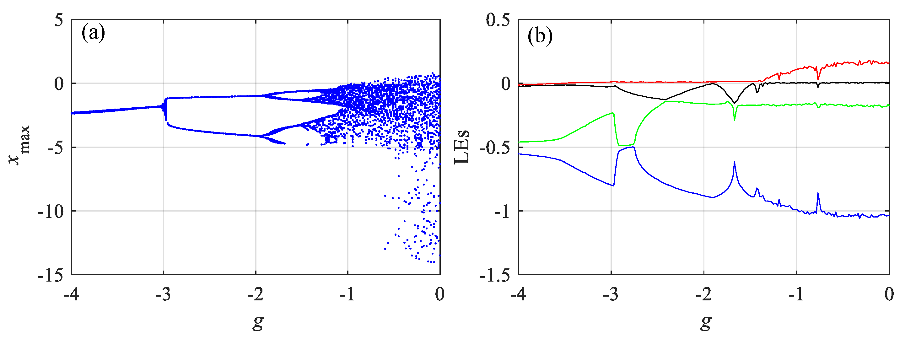
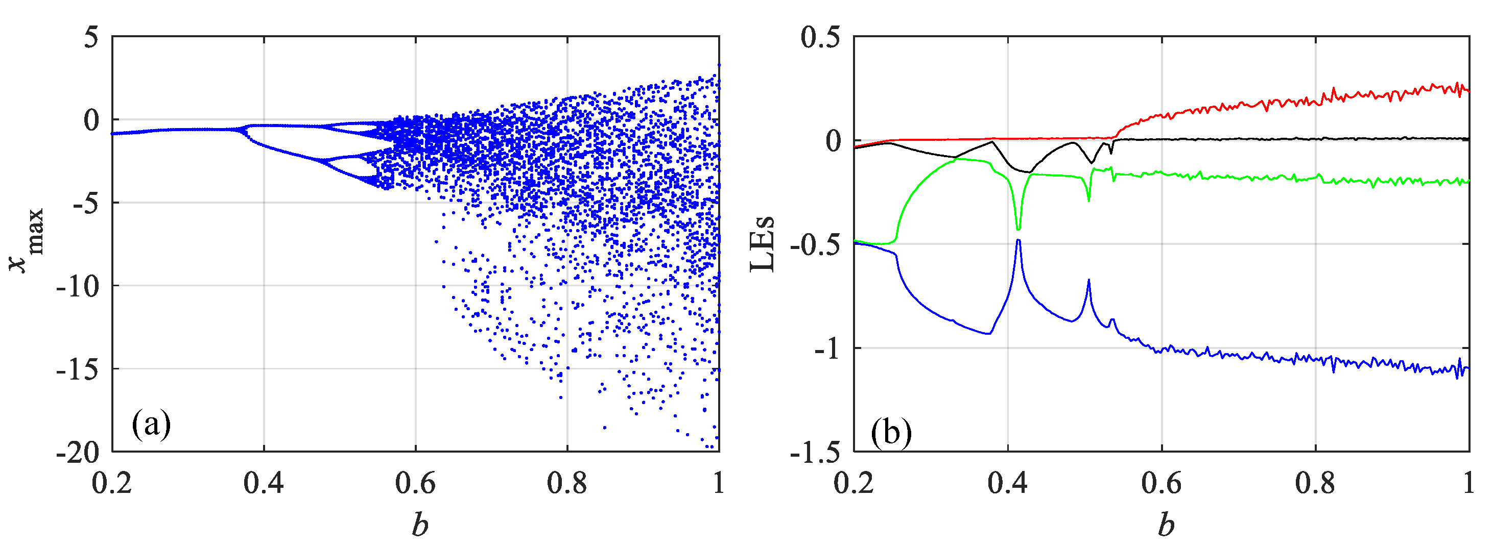
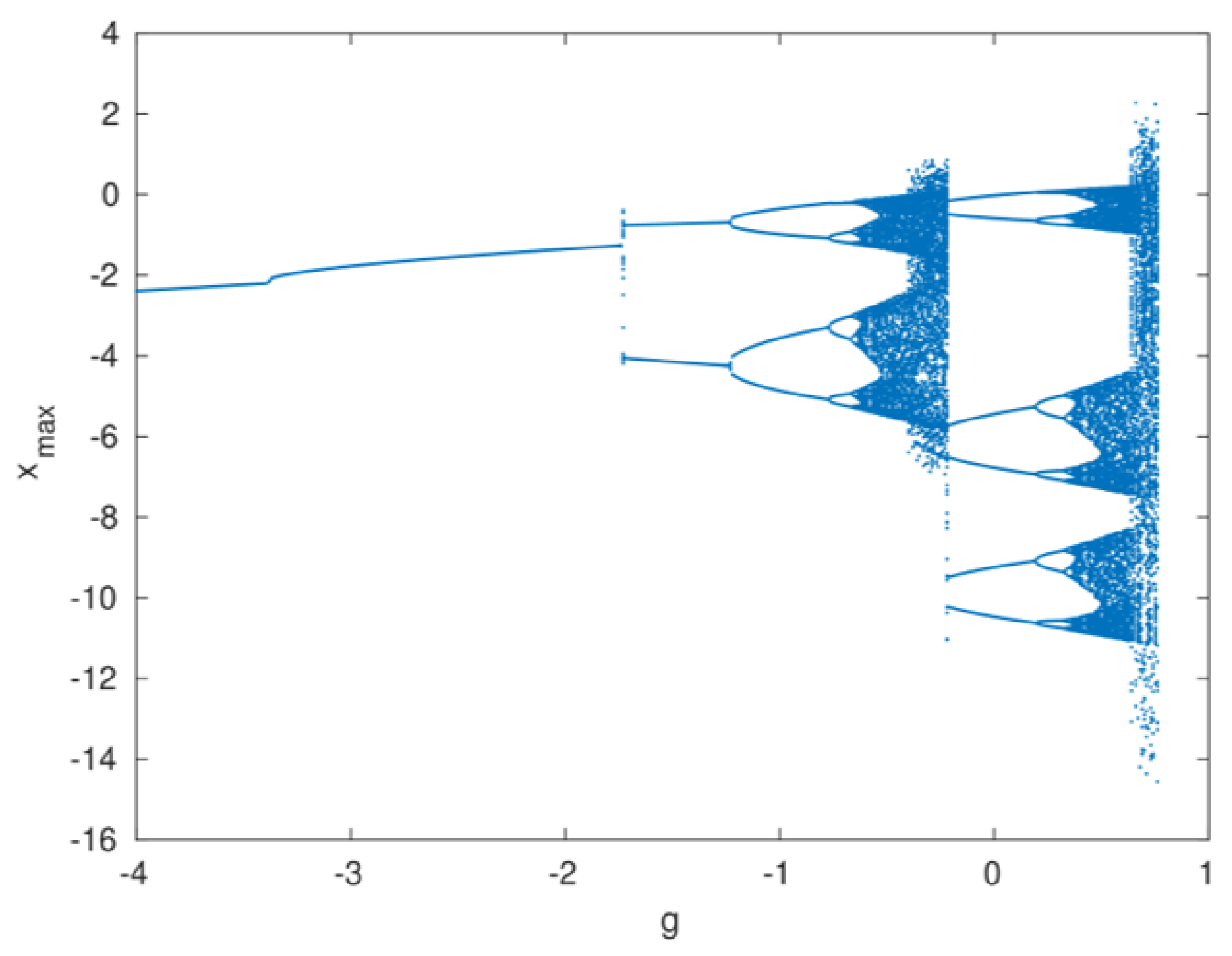
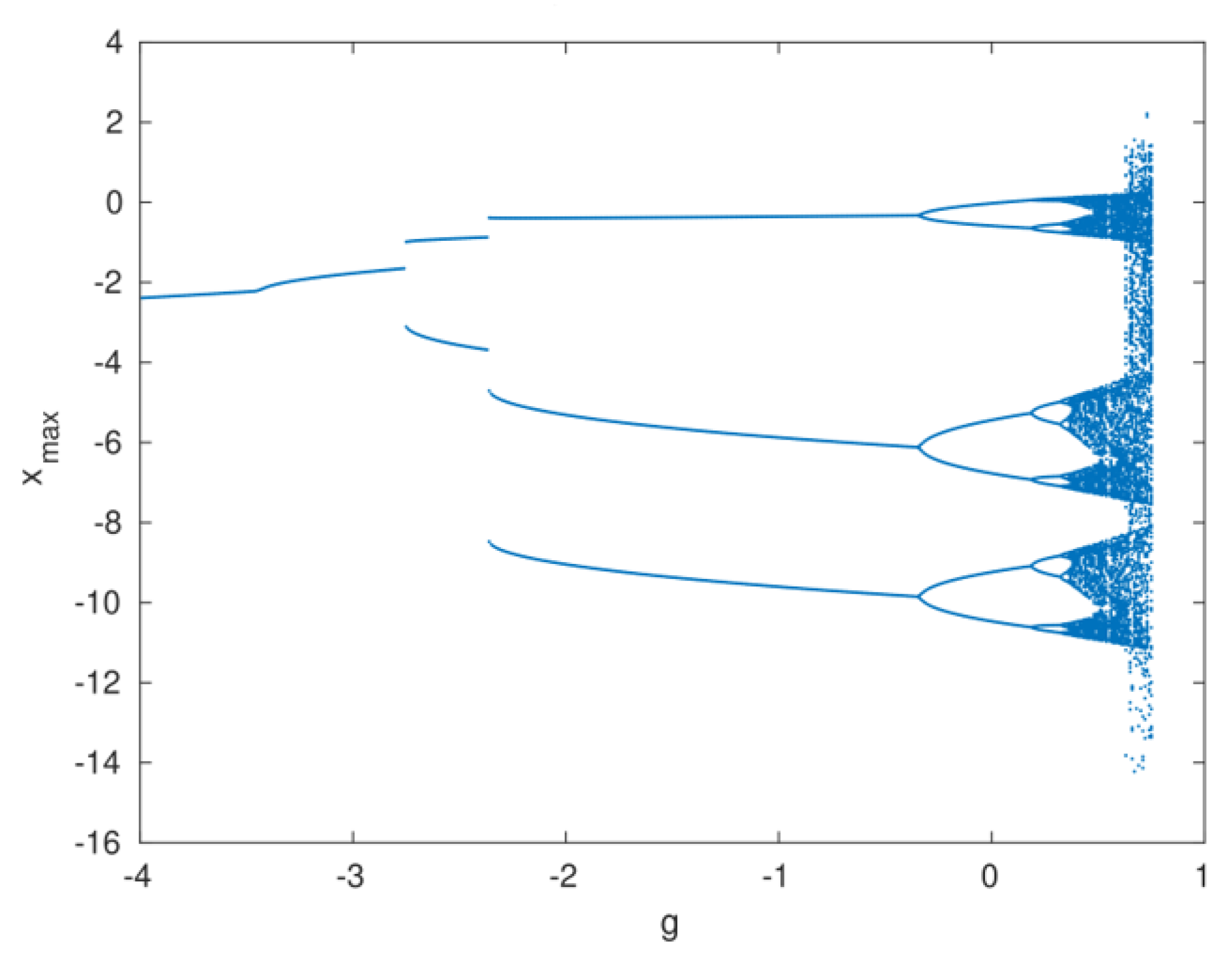
2.1. Dynamical Analysis

Since $bg\le 0$, values of $g$ less than, and equal to zero are chosen. Taking $a=1.05, b=0.7, c=0.19, e=1.37, f=1.79$, setting the initial conditions as $\left[x_0,y_0,z_0,w_0\right]=\left[-0.1,2.05,-1,-3.55\right]$, and varying the system parameter $g$ from −4 to 0 with a step size of 0.016, the bifurcation diagrams and Lyapunov exponents (LEs) of the system with $g$ are as shown in Figure 1. As shown in Figure 1a, the system enters chaos with “period-doubling bifurcation.” Phase diagrams with $b=0.7$ and different $g$ are shown in Figure 2. When $g=-3.5$, the attractor is convergent. Of course, this is not a typical period-doubling bifurcation since “periodic one” is actually convergent. When $g=-2.5$ and $g=-1.5$, the attractor is periodic, and when $g=-0.15$, the attractor is chaotic. Moreover, Figure 1b shows that the maximum LEs of the system increase with the increase in $g$. Thus, the system has rich dynamics with the variation of the constant $g$.

Let $a=1.05, c=0.19, e=1.37, f=1.79, g=-0.15$, and vary the system parameter $g$ from 0.2 to 1 with a step size of 0.0032. By setting the initial conditions as $\left[x_0,y_0,z_0,w_0\right]=\left[-0.1,2.05,-1,-3.55\right]$, the bifurcation diagram and LEs of the system are as illustrated in Figure 3. As can be observed in Figure 3a, the system enters chaos with period-doubling bifurcation, and the size of the attractors increases with the parameter $b$, which is also verified by the phase diagrams shown in Figure 4. Meanwhile, the maximum LEs increase with parameter $b$, thus suggesting that the system with a larger parameter has a relatively higher complexity.

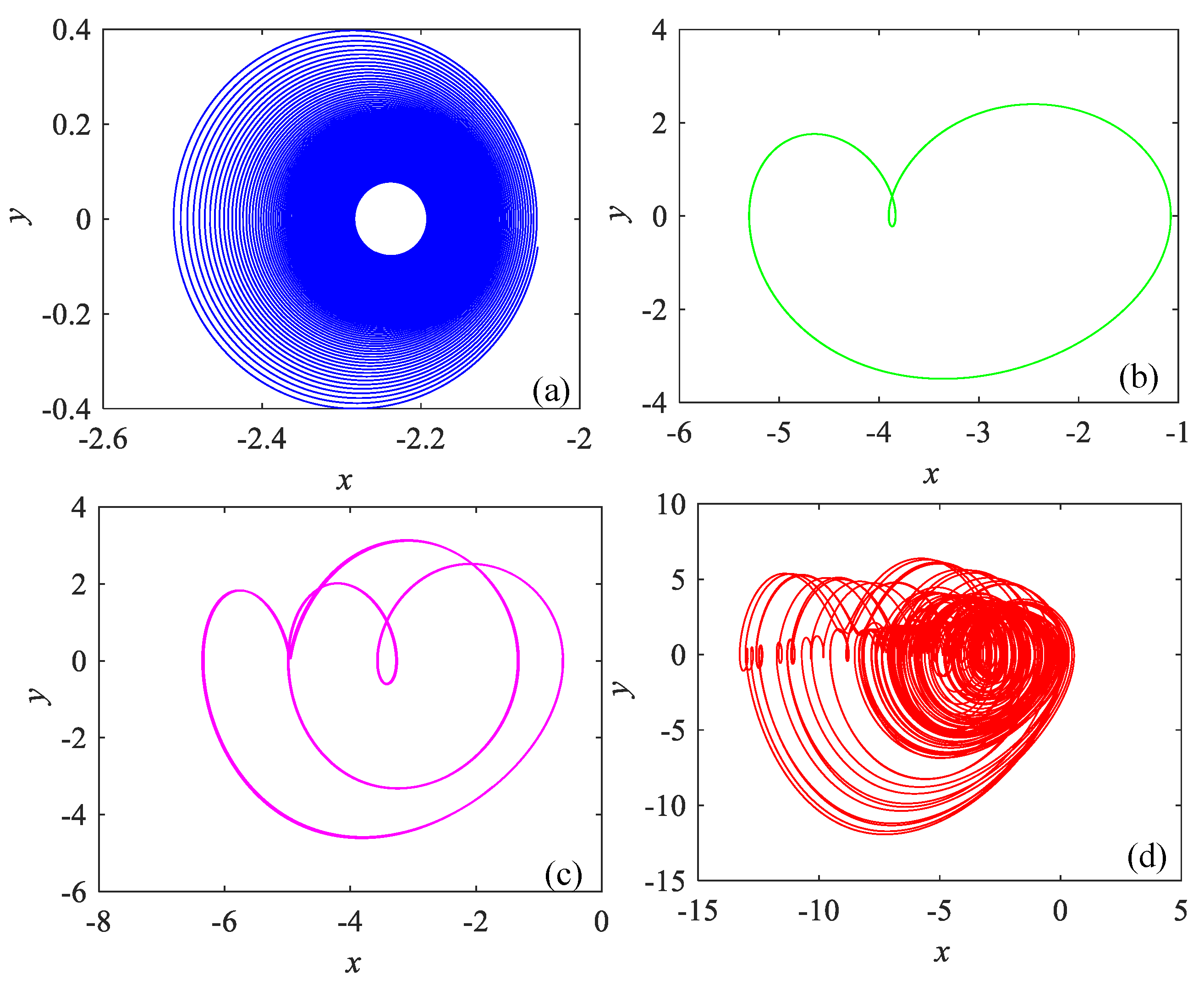
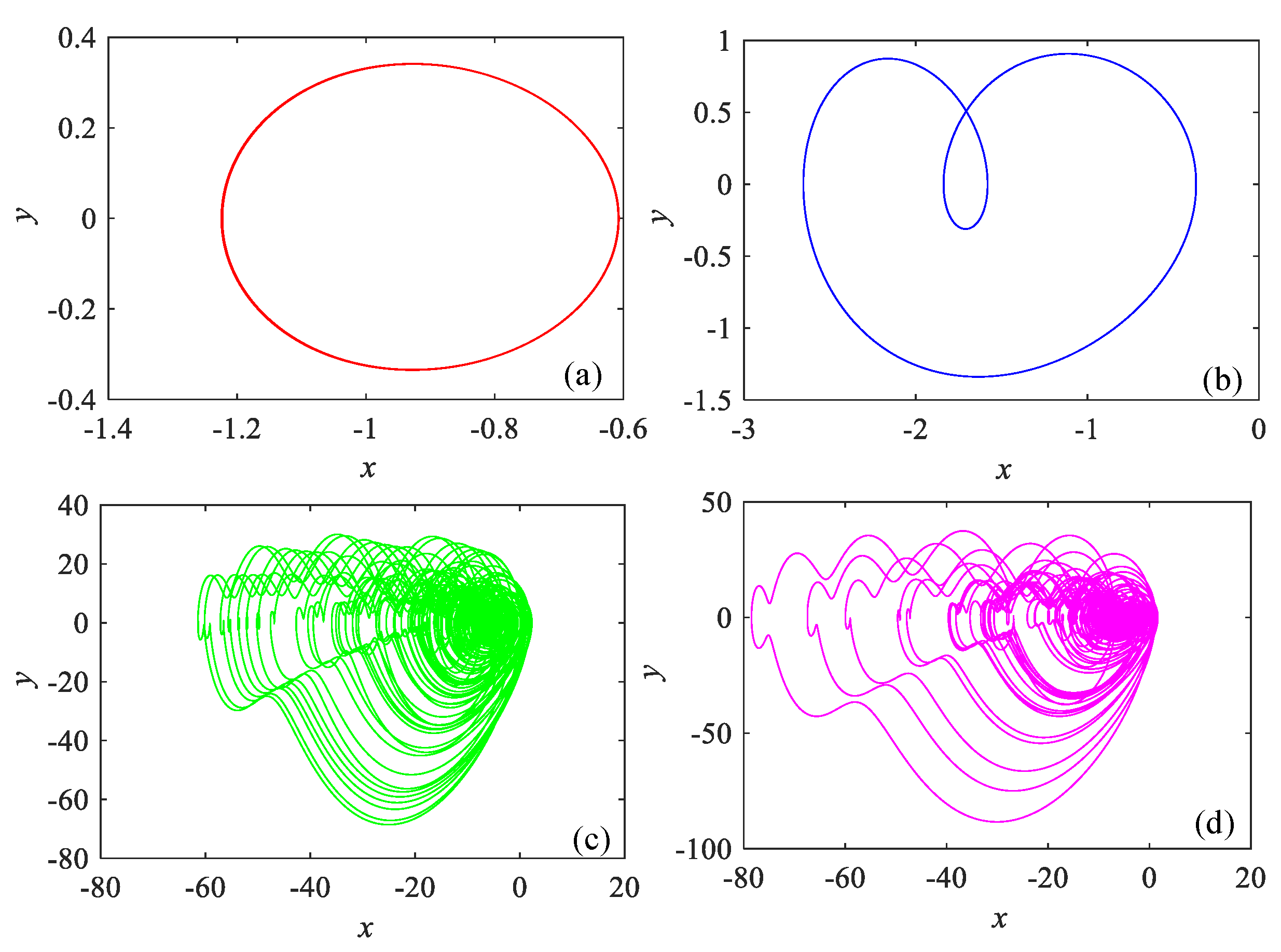
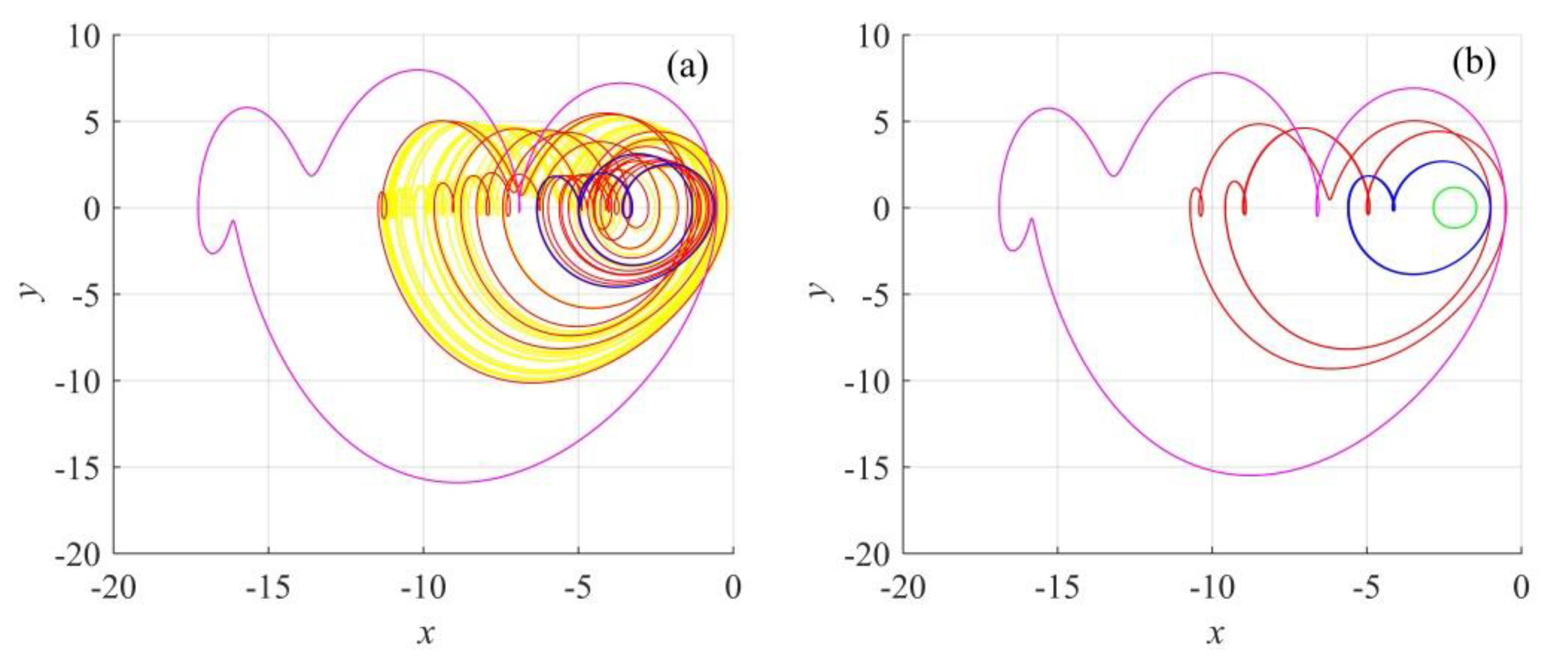
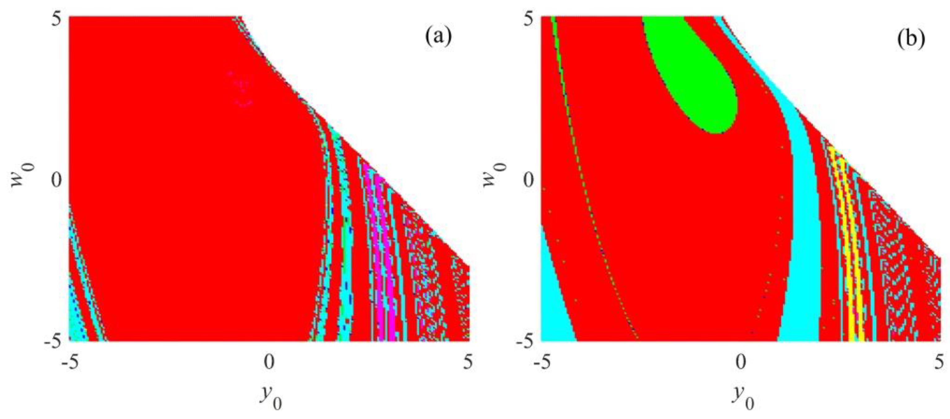
2.2. Coexisting Attractors

By establishing $a=1.05$, $b=0.7$, $c=0.19$, $e=1.37$, and $f=1.79$, the coexisting attractors in the proposed jerk system are investigated in this section. When the system parameter $g$ is set as $-1.5$ and the initial conditions are set as $\left[x_0,y_0,z_0,w_0\right]=\left[-0.1,2.05,-1,-3.55\right]$, the yellow chaotic attractor is as shown in Figure 5a. Meanwhile, the coexisting percircles are also observed, where the red, blue and magenta color periodic circles have the initial conditions $\left[x_0,y_0,z_0,w_0\right]=\left[-0.1,2,-1,-4\right]$, $\left[x_0,y_0,z_0,w_0\right]=\left[-0.1,-0.2,-1,-0.4\right]$, and $\left[x_0,y_0,z_0,w_0\right]=\left[-0.1,2.05,-1,-3.55\right]$, respectively. On the other hand, if $g=-2$, the multiple coexisting periodic attractors are as shown in Figure 5b. In this case, the initial conditions for the green, red, blue and magenta color periodic circles are $\left[x_0,y_0,z_0,w_0\right]=\left[-0.1,-0.9,-1,3.25\right]$, $\left[x_0,y_0,z_0,w_0\right]=\left[-0.1,2,-1,-4\right]$, $\left[x_0,y_0,z_0,w_0\right]=\left[-0.1,-0.2,-1,-0.4\right]$, and $\left[x_0,y_0,z_0,w_0\right]=\left[-0.1,2.05,-1,-3.55\right]$, respectively. To further explore the coexisting dynamics, the basin attraction of the system with $g=-0.15$ and $g=-2$ is as presented in Figure 6, where $y_0$ and $w_0$ vary from −5 to 5 with a step size of 0.05. As can be seen, the proposed jerk system has coexisting attractors.

In Equation (1), the coefficient of $y^2$ is considered to have a negative value, and in this condition a series of period-doubling cascades is detected, as displayed in Figure 7 and Figure 8. To plot the bifurcation diagrams, the system parameter $g$ is considered within the interval [$-4,0.75$]. The forward and backward results are illustrated in Figure 7 and Figure 8, respectively. As can be observed in these figures, chaotic, periodic, and period-doubled states exist in the forward bifurcation, while only periodic states exist in the backward bifurcation, which shows multiple attractors.

2.3. Hidden Chaotic Attractor

Self-excited and hidden oscillations in which one or both may occur in chaotic flows are defined by the following definition:

Definition 1.

“If basin of attraction in a system intersects with any open neighborhood of equilibrium, then the attractor of the system is a self-excited attractor; otherwise, it is a hidden attractor [43].”

By considering $f\left(x,y,z,w,t\right)=0$ in the proposed system as shown in Equation (1), and choosing $b$ and $g$ nonzero parameters with the same signs, then there are no equilibria. Hence, in this situation and according to Definition 1, the attractor of the proposed system in Equation (1) is hidden.

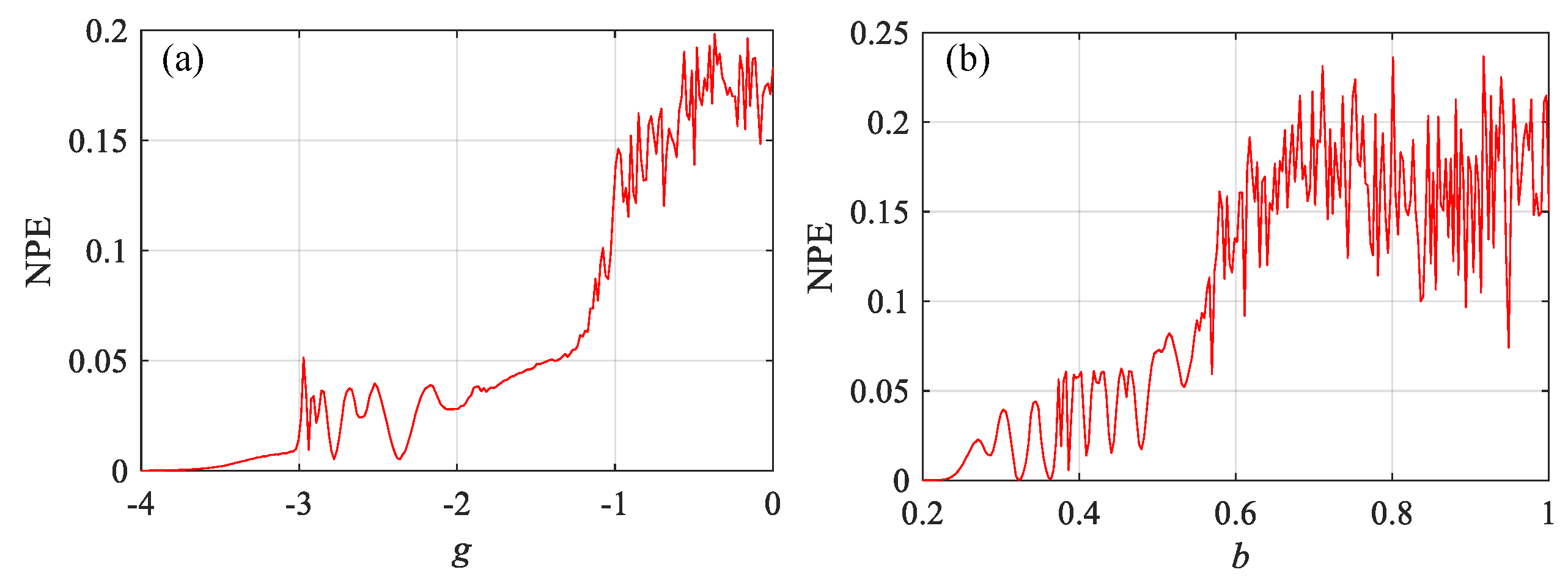
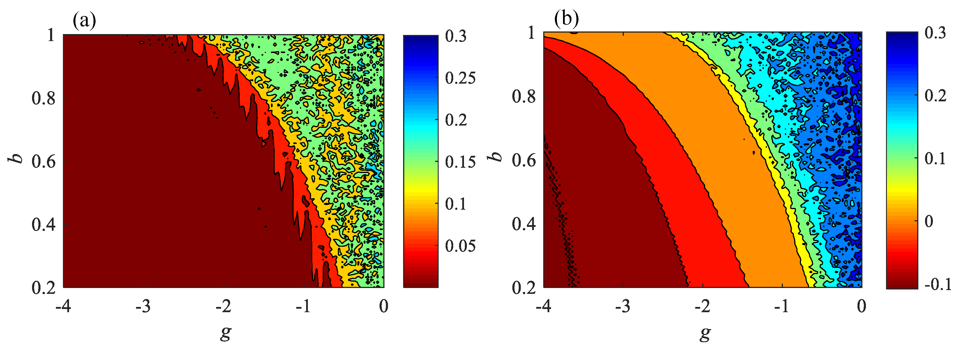
3. Complexity Analysis

In this section, the complexity of the analyzed four-dimensional chaotic system is measured by employing a multiscale C₀ (MC₀) complexity measure. From a mathematical point of view, with the given time series $\left\{x\left(n\right),n=0,1,2,\dots ,N-1\right\},$ its current part must be removed by

$$x\left(n\right)=x\left(n\right)-\overline{x},$$

(2)

where $\overline{x}=\frac{1}{N}{\sum }_{n=0}^{N-1}x\left(n\right)$. Then, the spectral content of the time series can be estimated by the Fourier transform as

$$X\left(k\right)={\sum }_{n=0}^{N-1}x\left(n\right)e^{-j\frac{2\pi }{N}nk},$$

(3)

being $\mathrm{k}=0,1,2,\dots ,\mathrm{N}-1$. In this step, the irregular part of the series is moved. Thus, the first step is to calculate the threshold value $G_N=\frac{1}{N}{\sum }_{k=0}^{N-1}{\left|X\left(k\right)\right|}^2$.

The second step is to introduce a control parameter r, and to redefine the frequency as

$$\tilde{X}\left(k\right)=\{\begin{array}{cc}X\left(k\right)& if {\left|X\left(k\right)\right|}^2>r{G}_N\\ 0& if {\left|X\left(k\right)\right|}^2\le r{G}_N\end{array}.$$

(4)

Finally, the inverse Fourier transform of the new frequency $\tilde{X}\left(k\right)$ is given by

$$\tilde{x}\left(n\right)=\frac{1}{N}{\sum }_{k=0}^{N-1}\tilde{X}\left(k\right)e^{\frac{j2\pi nk}{N}},$$

(5)

where $n=0,1,\dots ,N-1.$ Clearly, $\tilde{x}\left(n\right)$ keeps the regular part of $x$($n$). The C₀ complexity measure is then estimated by obtaining the ratio between the summation of the irregular part and that of the original time series, i.e.,

$${\mathrm{C}}_0\left(x,r,N\right)=\frac{{{\displaystyle \sum }}_{n=0}^{N-1}{\left|x\left(n\right)-\tilde{x}\left(n\right)\right|}^2}{{{\displaystyle \sum }}_{n=0}^{N-1}{\left|x\left(n\right)\right|}^2}.$$

(6)

To get a better measure result, the ${\mathrm{MC}}_0$ complexity measure algorithm [25] is employed, which is given by

$$y^s\left(j\right)=\frac{1}{s}{{\displaystyle \sum }}_{i=\left(j-1\right)s+1}^{js}x\left(i\right),$$

(7)

where $1\le j\le N/s$, ⌊∙⌋ is the floor function, and s is the scale factor. As a result, the ${\mathrm{MC}}_0$ measure is given as

$${\mathrm{MC}}_0\left(x,r,s,N\right)=\frac{1}{s}{{\displaystyle \sum }}_{i=1}^s{C}_0\left(y^s,r,N\right).$$

(8)

In the present work, the maximum scale factor is chosen as $s=20$. Figure 9 and Figure 10 show the MC₀ complexity analysis results of the proposed system as functions of the parameters $g$ and $b$. To obtain these results, the initial condition of the system is [x₀, y₀, z₀, w₀] = [−0.1, −0.2, −0.3, −0.4] and time series of 20,000 points from the variable $x$($n$) is used, where the first 10,000 points are removed. In Figure 9, the parameter $g$ varies from −4 to 0 with a step size of 0.016. In Figure 10, the parameter $b$ increases from 0.2 and 1 with an increment of 0.0032. It should be noted in Figure 9 and Figure 10 that the complexity increases with the parameters $g$ and $b$ and maintains steadiness at the end. In Figure 10, the parameter $g$ varies from −4 to 0 with a step size of 0.04, while the parameter $b$ varies from 0.2 to 1 with a step size of 0.008. The MC₀ and the maximum LEs-based contour plots show that the system has higher complexity in the right size of the parameter plane, thus suggesting that the system is chaotic or has higher complexity for the larger values of $g$. Meanwhile, when $g>-3$, the system has a wider complexity region with a larger parameter $b$. Thus, in real applications, the system can have a higher complexity with relatively larger parameters $g$ and $b$.

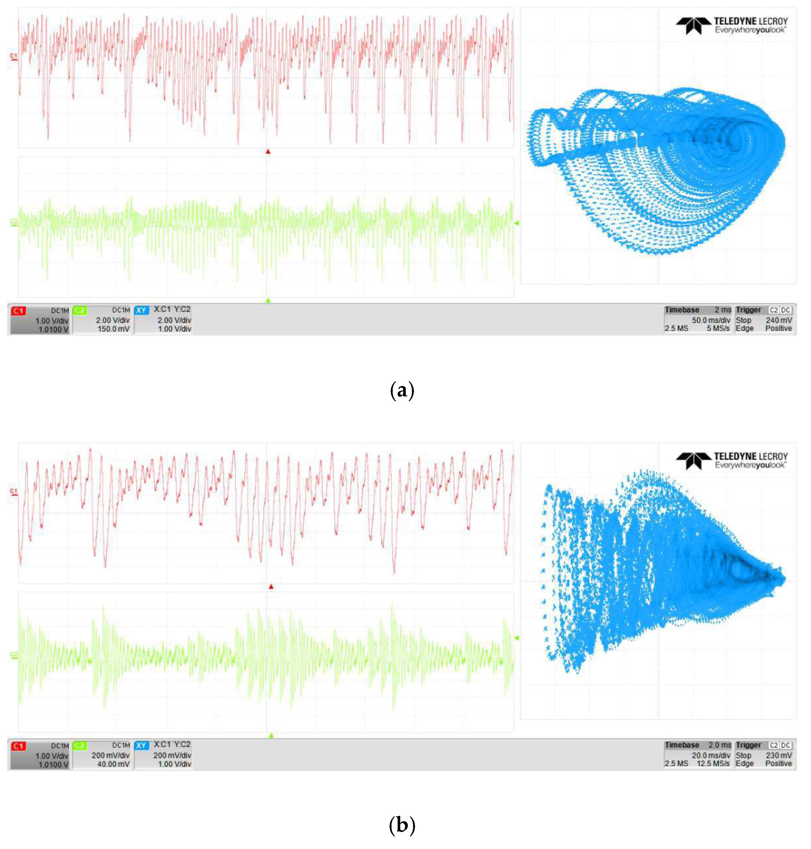
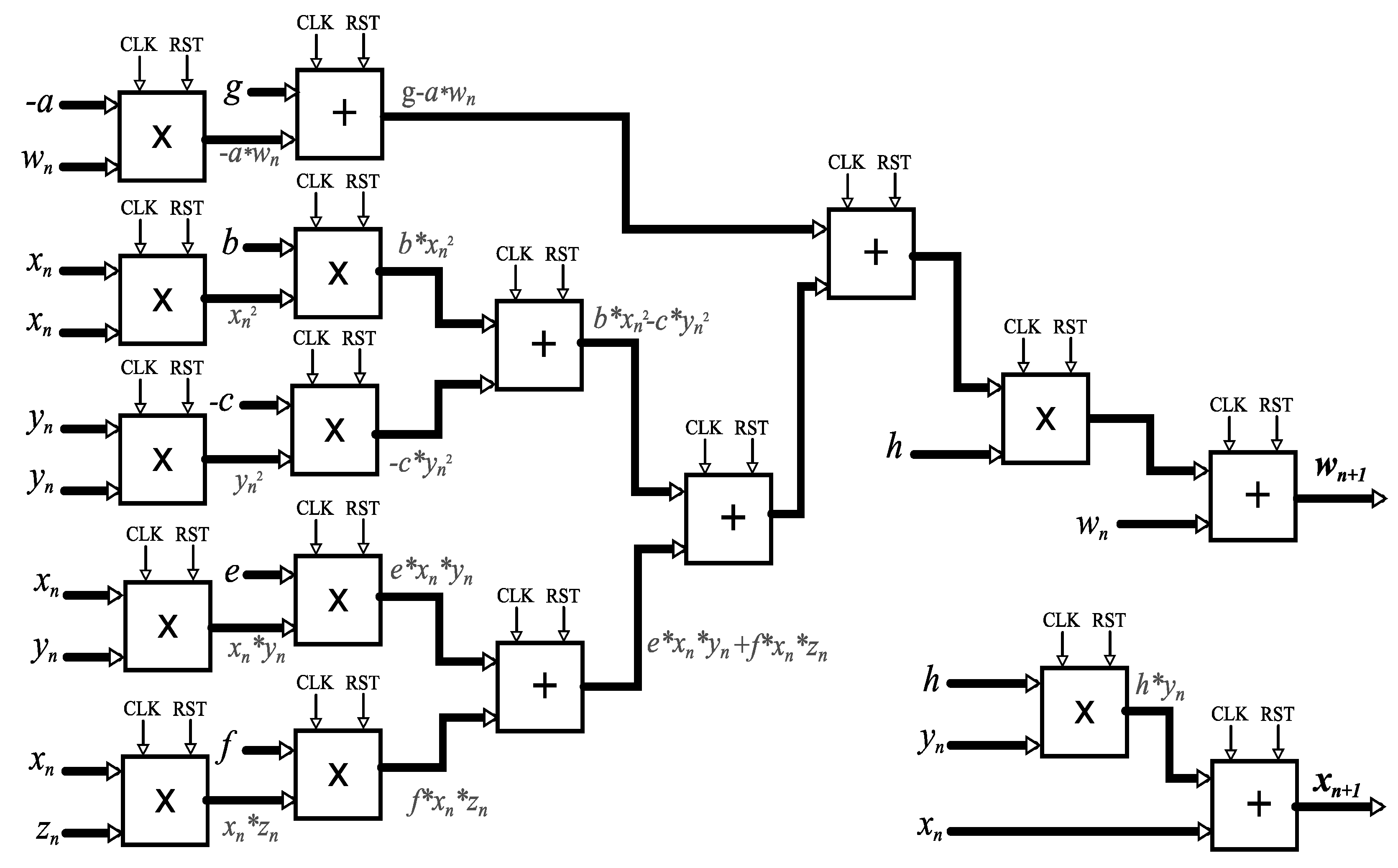
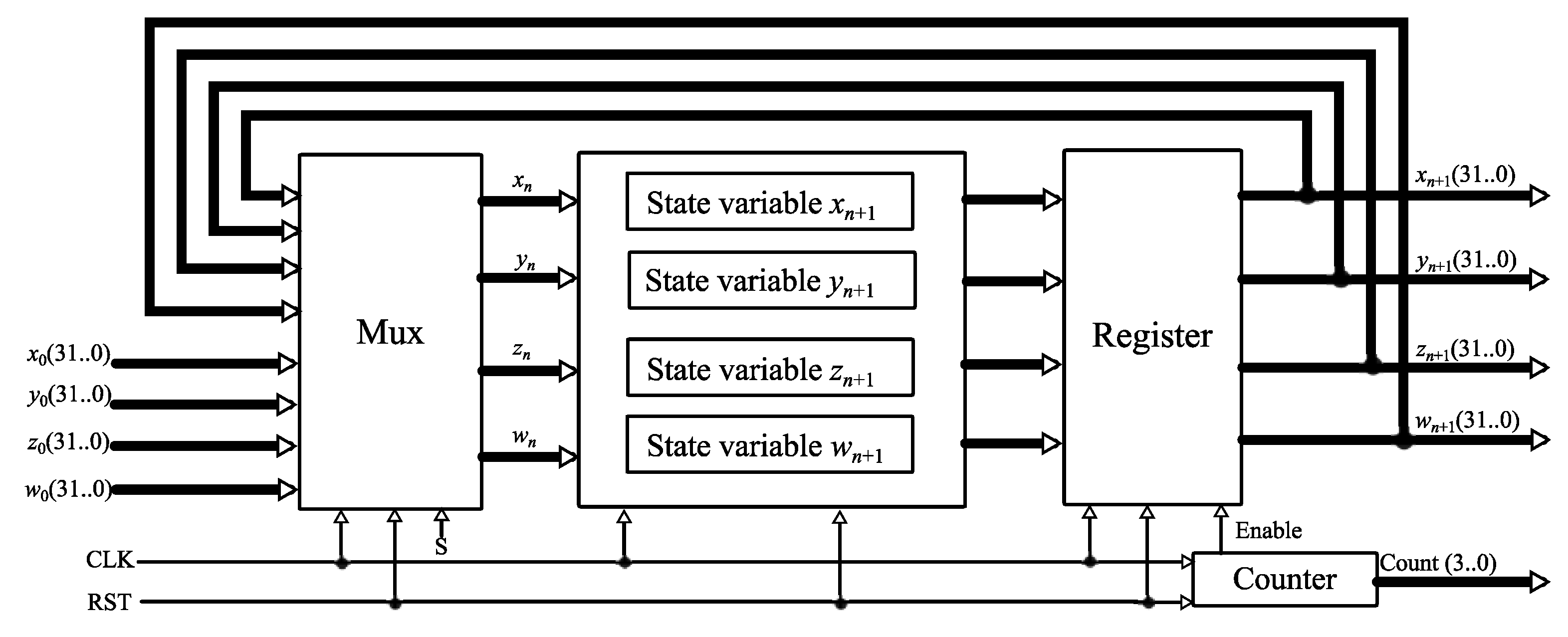
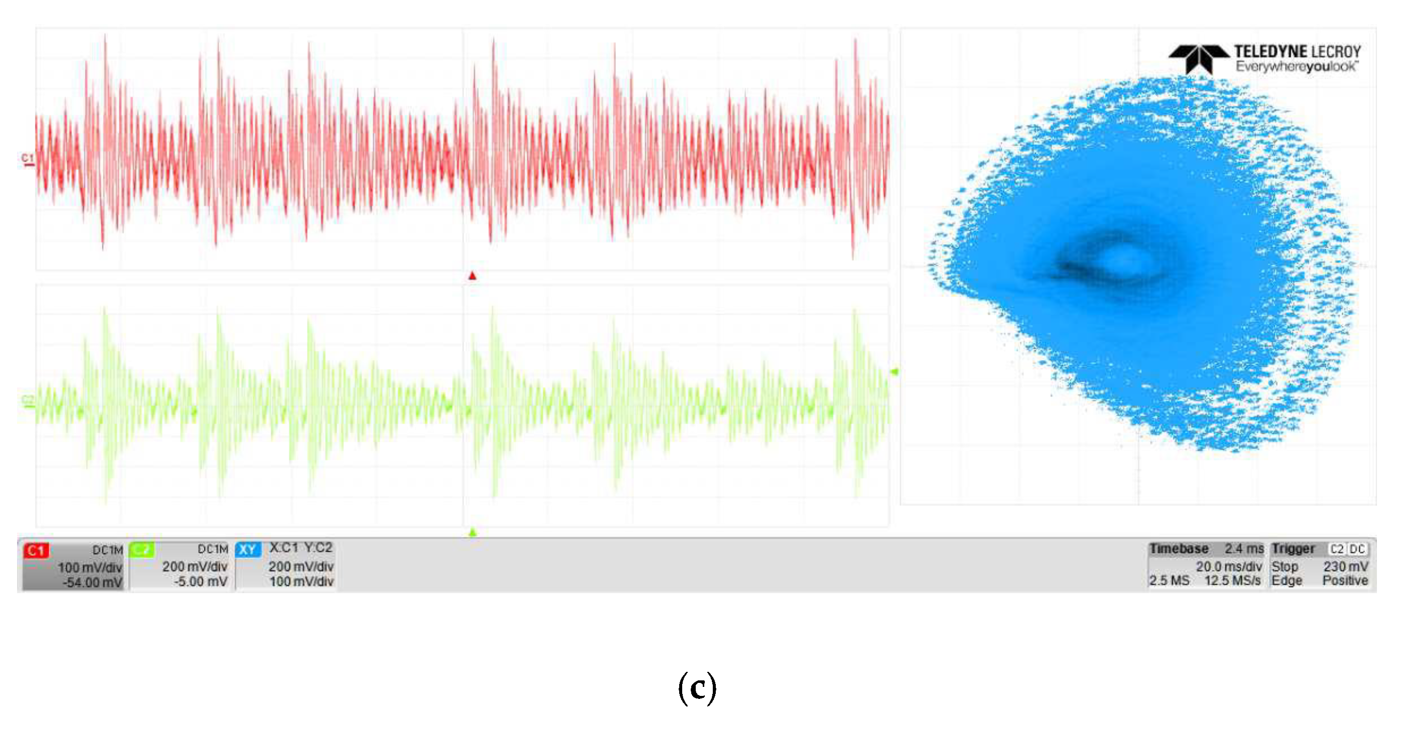
4. FPGA Implementation

Following the methodology provided in [54,55], the FPGA implementation of the proposed system in Equation (1) is completed by applying the forward Euler method, and it is carried out on the discretization of the chaotic system, such that

$$\begin{array}{c}{x}_{n+1}=x_n+h\left(y_n\right),\\ y_{n+1}=y_n+\left(h{z}_n\right),\\ z_{n+1}=z_n+h\left(w_n\right),\\ w_{n+1}=w_n+h\left(-a{w}_n+b{x}_n{}^2-c{y}_n{}^2+e{x}_n{y}_n+f{x}_n{z}_n+g\right),\end{array}$$

(9)

where $h$ is the step size, and the initial condition $\left[x\left(0\right), y\left(0\right), z\left(0\right), w\left(0\right)\right]=\left[0,-1, 0,-1.5\right]$. Fixed-point operation is used for the hardware implementation to obtain higher speed and a lower cost [75]. Furthermore, the N-bits 2′s complement representation is used because it is able to represent numbers over the range $\left\{-2^{N-1},2^{N-1}-1\right\}$. In the present work, 32 bits are used, where the most significant bit represents the sign, 10 bits are used to express the integer part, and 21 bits to express the fractional part.

From Equation (3), it is possible to identify the algebraic operations and perform the VHDL design. Figure 11 shows the block connection of the state variables $x_{n+1}$ and $w_{n+1}$, where the adder and multiplier blocks present clock (CLK) and reset (RST) signals to make the system synchronous [55]. By following the same methodology, all blocks connecting the state variables $y_{n+1}$ and $z_{n+1}$ are also designed.

Figure 12 shows the complete implementation of the system. Briefly, a multiplexer (MUX) is used to obtain the values of $x_n, y_n, and z_n,$ where at the first iteration, the outputs are equal to the initial conditions. While only three clock cycles are required to calculate the values of $x_{n+1}$, $y_{n+1}$, and $z_{n+1}$, it takes seven clock cycles to obtain the value of $w_{n+1}$. Therefore, to obtain the results of the state variables at the same instant of time, the Enable signal connected to the register is activated every eight clock cycles.

Finally, it should be noted that this work is based on using the FPGA Cyclone IV GX FPGA DE2i–150 from Altera and the digital-to-analog converter DAS1612. Figure 13 shows the experimental results and

Table 1. FPGA resources used for the real-time implementation of the proposed system.

Resources	Used
Total logic elements	1652/149,760 (1%)
Total registers	946
Total pins	25/508 (5%)
Total virtual pins	0
Total memory bits	192/6, 635, 520 (<1%)
Embedded multiplier 9-bit elements	92/720 (13%)
Latency	105.9 ns

lists the used resources. As can be seen in this table, the latency achieved is equal to 105.9 ns.

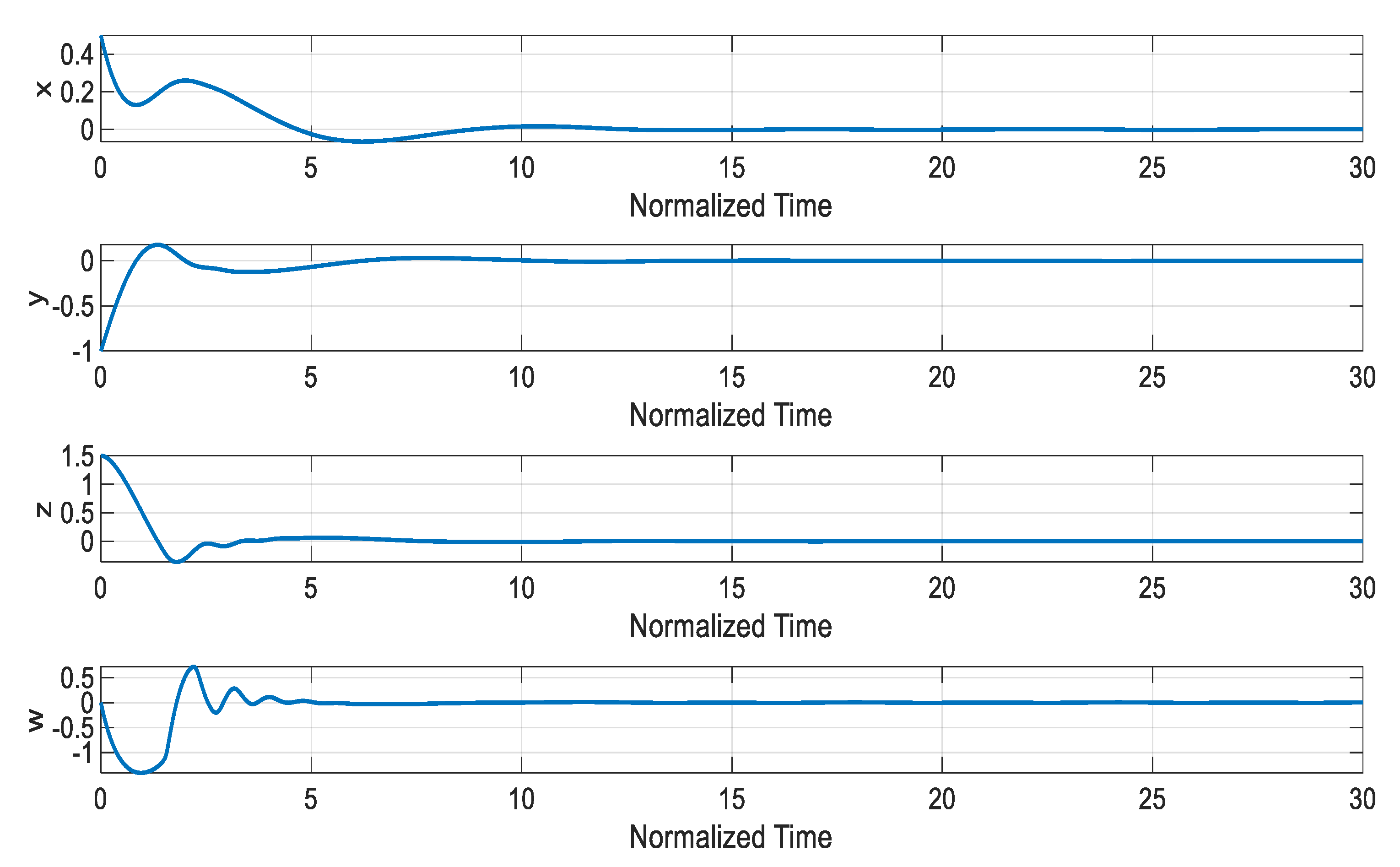
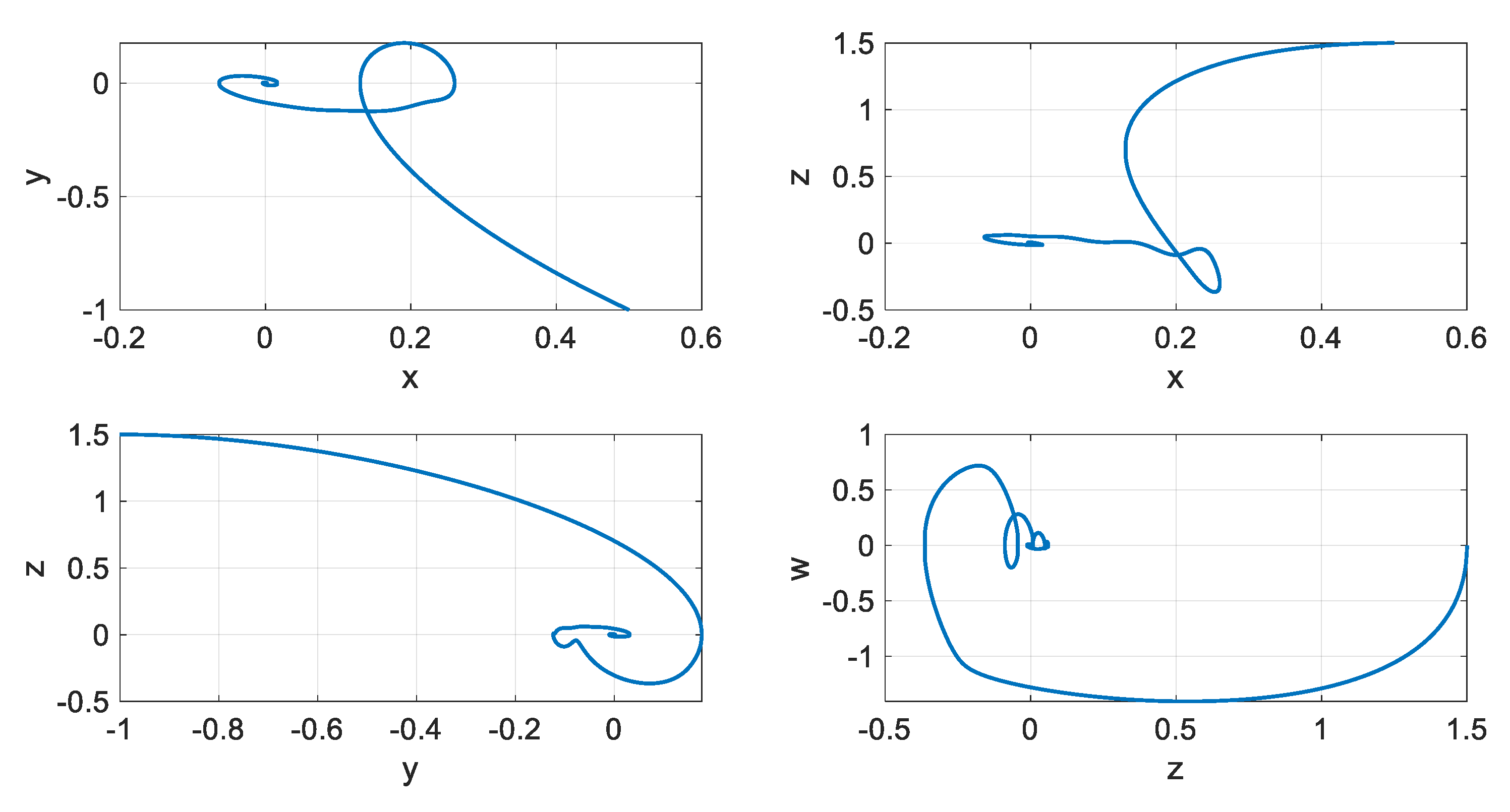
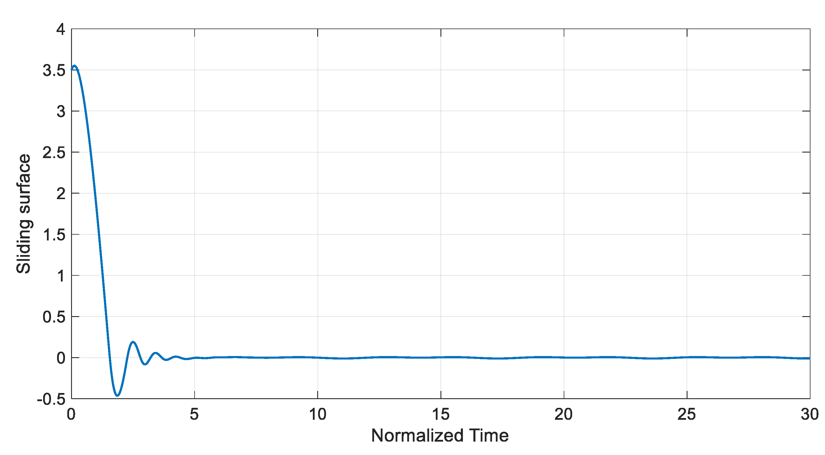
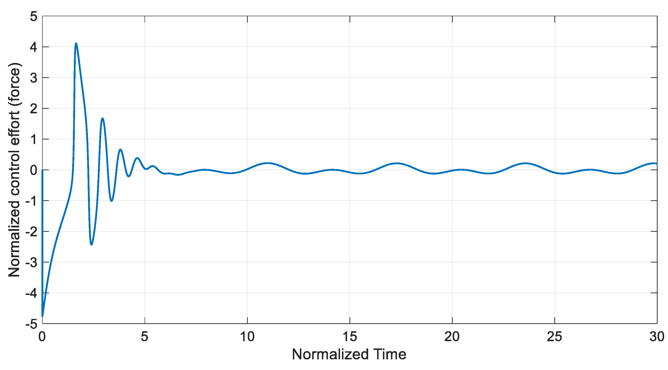
5. Controller Design

By defining $x_1=x,x_2=y,x_3=z,x_4=w,$ the state space of the proposed system in the presence of a disturbance is described as follows:

$$\{\begin{array}{ll}{\dot{x}}_i=f_i\left(x\right),& i=1,2,3\\ {\dot{x}}_4=f_4\left(x\right)+u+d\left(t\right),& \\ y=x_1,& \end{array}$$

(10)

where $f_i\left(x\right)=x_{i+1}$ for $i=1,2,3,f_4\left(x\right)=-a{x}_4+b{x}_1^2-c{x}_2^2+e{x}_1{x}_2+f{x}_1{x}_3+g,$ and $d\left(t\right)$ consists of an external disturbance.

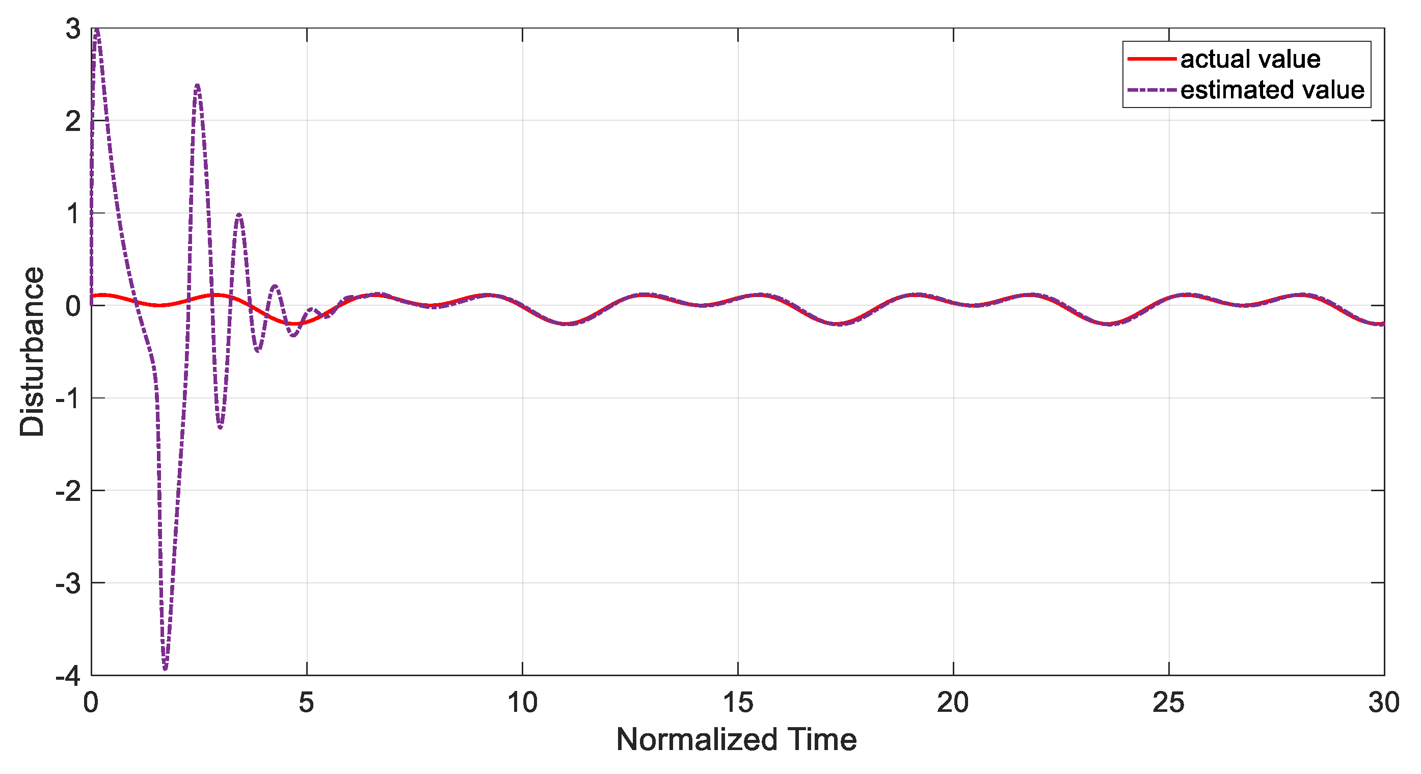
Disturbance Observer-Based SMC

A nonlinear disturbance observer is used to monitor external disturbances. The tracking error of the system is given by

$$e_i=x_i-x_{d\_i},$$

(11)

where $x_{d\_i}\mathrm{is}$ the desired state. The sliding mode function for SMC is considered as

$$S=c_1{e}_1+c_2{\dot{e}}_1+c_3{\ddot{e}}_1+c_4\dot{e_1},$$

(12)

where $c_1,c_2,c_3,c_4$ are design parameters and should be chosen as positive constants. As proposed in [76], a nonlinear disturbance observer to estimate the disturbance $\widehat{d}$ of the system described in Equation (10) is considered as

$$\begin{gathered} \dot{z}=\dot{\widehat{d}}-\frac{\partial p\left(x\right)}{\partial x}\dot{x}=-l\left(x\right)z-l\left(x\right)\left(p\left(x\right)+f_4\left(x\right)+u\right), \\ \widehat{d}=z+p\left(x\right), \end{gathered}$$

(13)

where $p\left(x\right)$ is a function to be designed, and it is related to the observer gain function $l\left(x\right)$ as follows:

$$-l\left(x\right)=\frac{\partial p\left(x\right)}{\partial x}.$$

(14)

The parameter $\tilde{d}$ is introduced as

$$\tilde{d}=d-\widehat{d},$$

(15)

and then, according to [76], for the proposed disturbance observer, it can be obtained that

$$\dot{\tilde{d}}+\frac{\partial p\left(x\right)}{\partial x}\tilde{d}=0,$$

(16)

when the gain $l\left(x\right)$ or $p\left(x\right)$ is designed such that $l\left(x\right)>\beta >0$. In this condition, $\tilde{d}\left(t\right)$ is globally exponentially convergent to zero with a rate of $e^{-\beta t}$ as $t\to \infty$. The control input signal based on SMC with the disturbance observer is then designed as

$$\begin{array}{l}u=-\frac{1}{c_4}(c_1{x}_1+c_2{x}_2+c_3{x}_3+c_4{f}_4\left(x\right)-c_1{\dot{x}}_{d1}-c_2{\dot{x}}_{d2}-c_3{\dot{x}}_{d3}-c_4{\dot{x}}_{d4}+c_4\widehat{d}+\alpha \mathrm{sign}\left(s\right)+\frac{{\left|c_{4}s\right|}^2}{\beta \left(x\right)}),\end{array}$$

(17)

where $\alpha ,c_1,c_2,c_3$ and $c_4$ are design parameters, $\alpha >0$ and $c_1,c_2,c_3$, $c_4$ are chosen such that $c_1,c_2,c_3,{\mathrm{c}}_4\ne 0$. The stability of this controller is proved if the Lyapunov function candidate is given by

$$V\left(s,\tilde{d}\right)=\frac{1}{2}{s}^2+\frac{1}{2}{\tilde{d}}^2,$$

(18)

and the time derivative of the Lyapunov function candidate is as follows:

$$\dot{V}\left(s,\tilde{d}\right)=s\dot{s}+\tilde{d}\dot{\tilde{d}}.$$

(19)

Considering Equations (10), (12), and (16), Equation (19) expands to

$$\begin{gathered} \dot{V}=s\left(c_1\left(x_1-x_{d1}\right)+c_2\left(x_2-x_{d2}\right)+c_3\left(x_3-x_{d3}\right)+c_4\left(x_4-x_{d4}\right)\right)-\frac{\partial p\left(x\right)}{\partial x}{\tilde{d}}^2 \\ =s\left(\left(c_1\left(x_1-x_{d1}\right)+c_2\left(x_2-x_{d2}\right)+c_3\left(x_3-x_{d3}\right)+c_4(f_4\left(x\right)+u+d\left(t\right)-x_{d4}\right)\right)+ \\ \frac{\partial p\left(x\right)}{\partial x}{\tilde{d}}^2. \end{gathered}$$

(20)

Substituting Equation (17) into Equation (20), it is obtained that

$$\begin{array}{l}\dot{V}=s{c}_4\left(d-\widehat{d}\right)+\frac{\partial p\left(x\right)}{\partial x}{\tilde{d}}^2-s\alpha \mathrm{sign}\left(s\right)-\frac{{\left|c_{4}s\right|}^2}{\beta \left(x\right)}=s{c}_2\tilde{d}+\frac{\partial p\left(x\right)}{\partial x}{\tilde{d}}^2-s\alpha \mathrm{sign}\left(s\right)-\frac{{\left|c_{4}s\right|}^2}{\beta \left(x\right)}.\end{array}$$

(21)

By considering $\beta \left(x\right)=\frac{\partial p\left(x\right)}{\partial x}>0,\mathrm{it}\mathrm{can}\mathrm{be}\mathrm{then}\mathrm{obtained}\mathrm{that}$

$$\begin{gathered} \dot{V}\le \left|s{c}_4\right|\left|\tilde{d}\right|-\beta \left(x\right){\left|\tilde{d}\right|}^2-\frac{{\left|c_{4}s\right|}^2}{\beta \left(x\right)}-s\alpha \mathrm{sign}\left(s\right)=-{\left(\sqrt{\beta \left(x\right)}\left|\tilde{d}\right|-\frac{\left|c_{4}s\right|}{\sqrt{\beta \left(x\right)}}\right)}^2- \\ s\alpha \mathrm{sign}\left(s\right)\le -s\alpha \mathrm{sign}\left(s\right). \end{gathered}$$

(22)

This last equation confirms that $\dot{V}<0$ for any $s\ne 0,$ and this consequently guarantees the steady-state tracking performance.

6. Numerical Simulations

In the previous section, the robust controller was designed to suppress the chaotic behavior in the proposed system. The simulation of this control scheme is now presented and discussed. The system parameters are chosen as $a=1.05, b=0.7, c=0.19, e=1.37, f=1.79,\mathrm{and} g=0$. The initial conditions are considered as

$$IC=\left[x\left(0\right),y\left(0\right),z\left(0\right),\mathrm{w}\left(0\right)]=[0.5,-1,1.5,0\right].$$

(23)

Furthermore, the parameters of the disturbance observer-based sliding mode tracking control are considered as

$$c_1=2,c_2=1,c_3=3,c_4=1,p=x_4,l=15,\mathrm{and}\beta \left(x\right)=10.$$

(24)

The case in which the system is in the presence of unknown external disturbance is as follows:

$$d\left(t\right)=0.1\sin \left(t\right)+0.1\cos \left(2t\right).$$

(25)

Figure 14 and Figure 15 depict the stabilized states of the system. As illustrated in these figures, the states of the system converge to zero using the disturbance observer-based SMC even when there exist unknown time-varying disturbances. Furthermore, Figure 16 shows the time history of the sliding surface. Based on Figure 14 and Figure 16, it could be confirmed that the proposed controller stabilizes the system in a short period of time. The control input signal is shown in Figure 17. The bound of the control input has an appropriate value, which could be applied to a real system using common actuators. Moreover, values of the actual and estimated disturbances are displayed in Figure 18. As can be observed, the designed disturbance observer accurately estimates nonlinear disturbances in the system, and this method can dramatically improve the performance of the controller.

7. Conclusions

A four-dimensional chaotic jerk system with specific features was presented in this work. The complex dynamical behavior of the system was first investigated by making use of phase diagrams, bifurcation diagrams, and multiscale C₀ complexity. The obtained results show that the system presents chaotic behavior after a period-doubling bifurcation, as well as that its complexity increases with the parameters $g$ and $b$. The existence of coexisting attractors and hidden attractors in the proposed system was also verified. Moreover, to support the possible application of the system in real-world engineering processes, a FPGA-based implementation was described and confirmed. Finally, a robust control technique was designed, and its ability to suppress the chaotic behavior of the system in a short period of time, even in the presence of unknown time-varying disturbances, was proven through numerical simulations. As a future suggestion, engineering applications such as voice encryption of the proposed system could be studied.

References

1. Vaidyanathan, S.; Volos, C. Advances and Applications in Chaotic Systems; Springer: Berlin/Heidelberg, Germany, 2016. [Google Scholar]
2. Yousefpour, A.; Jahanshahi, H.; Munoz-Pacheco, J.M.; Bekiros, S.; Wei, Z. A fractional-order hyper-chaotic economic system with transient chaos. Chaos Solitons Fractals 2020, 130, 109400. [Google Scholar] [CrossRef]
3. Pham, V.T.; Volos, C.; Kapitaniak, T.; Jafari, S.; Wang, X. Dynamics and circuit of a chaotic system with a curve of equilibrium points. Int. J. Electron. 2017, 105, 385–397. [Google Scholar] [CrossRef]
4. Rajagopal, K.; Jahanshahi, H.; Varan, M.; Bayır, I.; Pham, V.-T.; Jafari, S.; Karthikeyan, A. A hyperchaotic memristor oscillator with fuzzy based chaos control and LQR based chaos synchronization. AEU Int. J. Electron. Commun. 2018, 94, 55–68. [Google Scholar] [CrossRef]
5. Munoz-Pacheco, J.; Zambrano-Serrano, E.; Volos, C.; Jafari, S.; Kengne, J.; Rajagopal, K. A new fractional-order chaotic system with different families of hidden and self-excited attractors. Entropy 2018, 20, 564. [Google Scholar] [CrossRef] [Green Version]
6. Jahanshahi, H.; Yousefpour, A.; Munoz-Pacheco, J.M.; Moroz, I.; Wei, Z.; Castillo, O. A new multi-stable fractional-order four-dimensional system with self-excited and hidden chaotic attractors: Dynamic analysis and adaptive synchronization using a novel fuzzy adaptive sliding mode control method. Appl. Soft Comput. 2020, 87, 105943. [Google Scholar] [CrossRef]
7. Eisencraft, M.; Attux, R.; Suyama, R. Chaotic Signals in Digital Communications; CRC Press: Boca Raton, FL, USA, 2018. [Google Scholar]
8. Jahanshahi, H.; Rajagopal, K.; Akgul, A.; Sari, N.N.; Namazi, H.; Jafari, S. Complete analysis and engineering applications of a megastable nonlinear oscillator. Int. J. Non-Linear Mech. 2018, 107, 126–136. [Google Scholar] [CrossRef]
9. Jahanshahi, H. Smooth control of HIV/AIDS infection using a robust adaptive scheme with decoupled sliding mode supervision. Eur. Phys. J. Spéc. Top. 2018, 227, 707–718. [Google Scholar] [CrossRef]
10. Yousefpour, A.; Bahrami, A.; Haeri Yazdi, M.R. Multi-frequency piezomagnetoelastic energy harvesting in the monostable mode. J. Theor. Appl. Vib. Acoust. 2018, 4, 1–18. [Google Scholar]
11. Yousefpour, A.; Vahidi-Moghaddam, A.; Rajaei, A.; Ayati, M. Stabilization of nonlinear vibrations of carbon nanotubes using observer-based terminal sliding mode control. Trans. Inst. Meas. Control 2019, 42, 1047–1058. [Google Scholar] [CrossRef]
12. Lai, Q.; Wang, L. Chaos, bifurcation, coexisting attractors and circuit design of a three-dimensional continuous autonomous system. Optik 2016, 127, 5400–5406. [Google Scholar] [CrossRef]
13. Wang, X.; Pham, V.-T.; Volos, C. Dynamics, circuit design, and synchronization of a new chaotic system with closed curve equilibrium. Complexity 2017, 2017, 1–9. [Google Scholar] [CrossRef] [Green Version]
14. Banerjee, T.; Biswas, D. Theory and experiment of a first-order chaotic delay dynamical system. Int. J. Bifurc. Chaos 2013, 23, 1330020. [Google Scholar] [CrossRef]
15. Bouali, S.; Buscarino, A.; Fortuna, L.; Frasca, M.; Gambuzza, L.V. Emulating complex business cycles by using an electronic analogue. Nonlinear Anal. Real World Appl. 2012, 13, 2459–2465. [Google Scholar] [CrossRef]
16. Jahanshahi, H.; Shahriari-Kahkeshi, M.; Alcaraz, R.; Wang, X.; Singh, V.P.; Pham, V.-T. Entropy Analysis and Neural Network-based Adaptive Control of a Non-Equilibrium Four-Dimensional Chaotic System with Hidden Attractors. Entropy 2019, 21, 156. [Google Scholar] [CrossRef] [Green Version]
17. Yousefpour, A.; Jahanshahi, H. Fast disturbance-observer-based robust integral terminal sliding mode control of a hyperchaotic memristor oscillator. Eur. Phys. J. Spéc. Top. 2019, 228, 2247–2268. [Google Scholar] [CrossRef]
18. Devaney, R. An Introduction to Chaotic Dynamical Systems; CRC Press: Boca Raton, FL, USA, 2018. [Google Scholar]
19. Jahanshahi, H.; Yousefpour, A.; Wei, Z.; Alcaraz, R.; Bekiros, S. A financial hyperchaotic system with coexisting attractors: Dynamic investigation, entropy analysis, control and synchronization. Chaos Solitons Fractals 2019, 126, 66–77. [Google Scholar] [CrossRef]
20. Chen, W.; Zhuang, J.; Yu, W.; Wang, Z. Measuring complexity using FuzzyEn, ApEn, and SampEn. Med. Eng. Phys. 2009, 31, 61–68. [Google Scholar] [CrossRef]
21. Larrondo, H.; González, C.; Martin, M.; Plastino, A.; Rosso, O.A. Intensive statistical complexity measure of pseudorandom number generators. Phys. A Stat. Mech. Appl. 2005, 356, 133–138. [Google Scholar] [CrossRef]
22. Staniczenko, P.P.A.; Lee, C.F.; Jones, N.S. Rapidly detecting disorder in rhythmic biological signals: A spectral entropy measure to identify cardiac arrhythmias. Phys. Rev. E 2009, 79, 011915. [Google Scholar] [CrossRef]
23. Wei, Q.; Liu, Q.; Fan, S.-Z.; Lu, C.-W.; Lin, T.Y.; Abbod, M.; Shieh, J.-S. Analysis of EEG via Multivariate Empirical Mode Decomposition for Depth of Anesthesia Based on Sample Entropy. Entropy 2013, 15, 3458–3470. [Google Scholar] [CrossRef] [Green Version]
24. En-Hua, S.; Zhi-Jie, C.; Fan-Ji, G. Mathematical foundation of a new complexity measure. Appl. Math. Mech. 2005, 26, 1188–1196. [Google Scholar] [CrossRef]
25. Wang, S.; He, S.; Yousefpour, A.; Jahanshahi, H.; Repnik, R.; Perc, M. Chaos and complexity in a fractional-order financial system with time delays. Chaos Solitons Fractals 2020, 131, 109521. [Google Scholar] [CrossRef]
26. He, S.; Sun, K.; Zhu, C.-X. Complexity analyses of multi-wing chaotic systems. Chin. Phys. B 2013, 22, 050506. [Google Scholar] [CrossRef]
27. Sun, K.-H.; He, S.-B.; He, Y.; Yin, L.-Z. Complexity Analysis of Chaotic Pseudo-Random Sequences Based on Spectral Entropy Algorithm. Acta Phys. Sin. 2013, 62, 010501. [Google Scholar]
28. Sharma, P.R.; Shrimali, M.D.; Prasad, A.; Kuznetsov, N.V.; Leonov, G. Control of multistability in hidden attractors. Eur. Phys. J. Spéc. Top. 2015, 224, 1485–1491. [Google Scholar] [CrossRef]
29. Lai, Q.; Chen, S. Generating Multiple Chaotic Attractors from Sprott B System. Int. J. Bifurc. Chaos 2016, 26, 1650177. [Google Scholar] [CrossRef]
30. Sprott, J.C.; Jafari, S.; Khalaf, A.J.M.; Kapitaniak, T. Megastability: Coexistence of a countable infinity of nested attractors in a periodically-forced oscillator with spatially-periodic damping. Eur. Phys. J. Spéc. Top. 2017, 226, 1979–1985. [Google Scholar] [CrossRef] [Green Version]
31. Bao, B.; Chen, M.; Bao, H.; Xu, Q. Extreme multistability in a memristive circuit. Electron. Lett. 2016, 52, 1008–1010. [Google Scholar] [CrossRef]
32. Bao, B.; Jiang, T.; Xu, Q.; Chen, M.; Wu, H.; Hu, Y. Coexisting infinitely many attractors in active band-pass filter-based memristive circuit. Nonlinear Dyn. 2016, 86, 1711–1723. [Google Scholar] [CrossRef]
33. Tlelo-Cuautle, E.; Rangel-Magdaleno, J.; Pano-Azucena, A.; Obeso-Rodelo, P.; Nuñez-Perez, J.-C. FPGA realization of multi-scroll chaotic oscillators. Commun. Nonlinear Sci. Numer. Simul. 2015, 27, 66–80. [Google Scholar] [CrossRef]
34. Muñoz-Pacheco, J.M.; Tlelo-Cuautle, E.; Toxqui-Toxqui, I.; Sánchez-López, C.; Trejo-Guerra, R. Frequency limitations in generating multi-scroll chaotic attractors using CFOAs. Int. J. Electron. 2014, 101, 1559–1569. [Google Scholar] [CrossRef]
35. Pham, V.-T.; Volos, C.; Jafari, S.; Kapitaniak, T. Coexistence of hidden chaotic attractors in a novel no-equilibrium system. Nonlinear Dyn. 2016, 87, 2001–2010. [Google Scholar] [CrossRef]
36. Pham, V.-T.; Jafari, S.; Volos, C.; Gotthans, T.; Wang, X.; Vo, D.H. A chaotic system with rounded square equilibrium and with no-equilibrium. Optik 2017, 130, 365–371. [Google Scholar] [CrossRef]
37. Jafari, S.; Sprott, J.; Golpayegani, S.M.R.H. Elementary quadratic chaotic flows with no equilibria. Phys. Lett. A 2013, 377, 699–702. [Google Scholar] [CrossRef]
38. Wei, Z. Dynamical behaviors of a chaotic system with no equilibria. Phys. Lett. A 2011, 376, 102–108. [Google Scholar] [CrossRef]
39. Pham, V.-T.; Akgul, A.; Volos, C.; Jafari, S.; Kapitaniak, T. Dynamics and circuit realization of a no-equilibrium chaotic system with a boostable variable. AEU-Int. J. Electron. Commun. 2017, 78, 134–140. [Google Scholar] [CrossRef]
40. Ren, S.; Panahi, S.; Rajagopal, K.; Akgul, A.; Pham, V.-T.; Jafari, S. A New Chaotic Flow with Hidden Attractor: The First Hyperjerk System with No Equilibrium. Z. Nat. A 2018, 73, 239–249. [Google Scholar] [CrossRef]
41. Lai, Q.; Chen, C.-Y.; Zhao, X.-W.; Kengne, J.; Volos, C. Constructing Chaotic System With Multiple Coexisting Attractors. IEEE Access 2019, 7, 24051–24056. [Google Scholar] [CrossRef]
42. Li, C.; Sprott, J.; Hu, W.; Xu, Y. Infinite Multistability in a Self-Reproducing Chaotic System. Int. J. Bifurc. Chaos 2017, 27, 1750160. [Google Scholar] [CrossRef]
43. Leonov, G.A.; Kuznetsov, N.V. Hidden attractors in dynamical systems. From hidden oscillations in Hilbert–Kolmogorov, Aizerman, and Kalman problems to hidden chaotic attractor in Chua circuits. Int. J. Bifurc. Chaos 2013, 23, 1330002. [Google Scholar] [CrossRef] [Green Version]
44. Leonov, G.; Kuznetsov, N.V.; Vagaitsev, V. Hidden attractor in smooth Chua systems. Phys. D Nonlinear Phenom. 2012, 241, 1482–1486. [Google Scholar] [CrossRef]
45. Kuznetsov, N.V.; Leonov, G.A.; Vagaitsev, V.I. Analytical-numerical method for attractor localization of generalized Chua’s system. IFAC Proc. Vol. 2010, 43, 29–33. [Google Scholar] [CrossRef]
46. Leonov, G.; Kuznetsov, N.V.; Vagaitsev, V. Localization of hidden Chua’s attractors. Phys. Lett. A 2011, 375, 2230–2233. [Google Scholar] [CrossRef]
47. He, S.; Sun, K.; Wu, X. Fractional symbolic network entropy analysis for the fractional-order chaotic systems. Phys. Scr. 2020, 95, 035220. [Google Scholar] [CrossRef]
48. Zhang, S.; Zeng, Y. A simple Jerk-like system without equilibrium: Asymmetric coexisting hidden attractors, bursting oscillation and double full Feigenbaum remerging trees. Chaos Solitons Fractals 2019, 120, 25–40. [Google Scholar] [CrossRef]
49. Kengne, J.; Signing, V.R.F.; Chedjou, J.C.; Leutcho, G.D. Nonlinear behavior of a novel chaotic jerk system: Antimonotonicity, crises, and multiple coexisting attractors. Int. J. Dyn. Control 2017, 6, 468–485. [Google Scholar] [CrossRef]
50. Elwakil, A.S.; Kennedy, M.P. Improved implementation of Chua’s chaotic oscillator using current feedback op amp. IEEE Trans. Circuits Syst. I 2000, 47, 76–79. [Google Scholar] [CrossRef] [Green Version]
51. Chiu, R.; Mora-Gonzalez, M.; Lopez-Mancilla, D. Implementation of a chaotic oscillator into a simple microcontroller. IERI Procedia 2013, 4, 247–252. [Google Scholar] [CrossRef] [Green Version]
52. De La Hoz, M.Z.; Acho, L.; Vidal, Y. An Experimental Realization of a Chaos-Based Secure Communication Using Arduino Microcontrollers. Sci. World J. 2015, 2015, 1–10. [Google Scholar] [CrossRef] [Green Version]
53. Yau, H.-T.; Wu, C.-H.; Liang, Q.-C.; Li, S.C. Implementation of optimal PID control for chaos synchronization by FPGA chip. In Proceedings of the 2011 International Conference on Fluid Power and Mechatronics, Beijing, China, 17–20 August 2011; pp. 56–61. [Google Scholar]
54. Shah, D.K.; Chaurasiya, R.B.; Vyawahare, V.A.; Pichhode, K.; Patil, M. FPGA implementation of fractional-order chaotic systems. AEU-Int. J. Electron. Commun. 2017, 78, 245–257. [Google Scholar] [CrossRef]
55. Tlelo-Cuautle, E.; De La Fraga, L.G.; Pham, V.-T.; Volos, C.; Jafari, S.; Quintas-Valles, A.D.J. Dynamics, FPGA realization and application of a chaotic system with an infinite number of equilibrium points. Nonlinear Dyn. 2017, 89, 1129–1139. [Google Scholar] [CrossRef]
56. Ya-Ming, X.; Li-Dan, W.; Shu-Kai, D. A memristor-based chaotic system and its field programmable gate array implementation. Acta Phys Sin. 2016, 65, 120503. [Google Scholar]
57. Wang, Q.; Yu, S.; Li, C.; Lu, J.; Fang, X.; Guyeux, C.; Bahi, J. Theoretical Design and FPGA-Based Implementation of Higher-Dimensional Digital Chaotic Systems. IEEE Trans. Circuits Syst. I Regul. Pap. 2016, 63, 401–412. [Google Scholar] [CrossRef] [Green Version]
58. Tuncer, T. The implementation of chaos-based PUF designs in field programmable gate array. Nonlinear Dyn. 2016, 86, 975–986. [Google Scholar] [CrossRef]
59. Dong, E.; Liang, Z.; Du, S.; Chen, Z. Topological horseshoe analysis on a four-wing chaotic attractor and its FPGA implement. Nonlinear Dyn. 2015, 83, 623–630. [Google Scholar] [CrossRef]
60. Tlelo-Cuautle, E.; Pano-Azucena, A.D.; Rangel-Magdaleno, J.; Carbajal-Gómez, V.H.; Rodriguez-Gomez, G. Generating a 50-scroll chaotic attractor at 66 MHz by using FPGAs. Nonlinear Dyn. 2016, 85, 2143–2157. [Google Scholar] [CrossRef]
61. Wang, Q.-X.; Yu, S.; Guyeux, C.; Bahi, J.; Fang, X.-L. Study on a new chaotic bitwise dynamical system and its FPGA implementation. Chin. Phys. B 2015, 24, 060503. [Google Scholar] [CrossRef]
62. Hua, Z.; Zhou, B.; Zhou, Y. Sine-Transform-Based Chaotic System With FPGA Implementation. IEEE Trans. Ind. Electron. 2018, 65, 2557–2566. [Google Scholar] [CrossRef]
63. Muñoz-Pacheco, J.M.; Tlelo-Cuautle, E.; Flores-Tiro, I.; Trejo-Guerra, R. Experimental Synchronization of two Integrated Multi-scroll Chaotic Oscillators. J. Appl. Res. Technol. 2014, 12, 459–470. [Google Scholar] [CrossRef]
64. Zambrano-Serrano, E.; Muñoz-Pacheco, J.M.; Gómez-Pavón, L.D.C.; Luis-Ramos, A.; Chen, G. Synchronization in a fractional-order model of pancreatic β-cells. Eur. Phys. J. Spéc. Top. 2018, 227, 907–919. [Google Scholar] [CrossRef]
65. Kosari, A.; Jahanshahi, H.; Razavi, S. An optimal fuzzy PID control approach for docking maneuver of two spacecraft: Orientational motion. Eng. Sci. Technol. Int. J. 2017, 20, 293–309. [Google Scholar] [CrossRef] [Green Version]
66. Kosari, A.; Jahanshahi, H.; Razavi, S.A. Optimal FPID Control Approach for a Docking Maneuver of Two Spacecraft: Translational Motion. J. Aerosp. Eng. 2017, 30, 04017011. [Google Scholar] [CrossRef]
67. Ma, Q.; Luo, W.; Jahanshahi, H.; Cavusoglu, U.; Akgul, A.; Lin, X. A novel s-box design algorithm and fuzzy-pid controller design for a 5-d burke–shaw system with hidden hyperchaos. System 2019, 2, 3. [Google Scholar] [CrossRef]
68. Jahanshahi, H.; Jafarzadeh, M.; Sari, N.N.; Pham, V.-T.; Huynh, V.; Nguyen, X.Q. Robot Motion Planning in an Unknown Environment with Danger Space. Electronics 2019, 8, 201. [Google Scholar] [CrossRef] [Green Version]
69. Sari, N.N.; Jahanshahi, H.; Fakoor, M. Adaptive Fuzzy PID Control Strategy for Spacecraft Attitude Control. Int. J. Fuzzy Syst. 2019, 21, 769–781. [Google Scholar] [CrossRef]
70. Mahmoodabadi, M.; Jahanshahi, H. Multi-objective optimized fuzzy-PID controllers for fourth order nonlinear systems. Eng. Sci. Technol. Int. J. 2016, 19, 1084–1098. [Google Scholar] [CrossRef] [Green Version]
71. Soradi-Zeid, S.; Jahanshahi, H.; Yousefpour, A.; Bekiros, S. King algorithm: A novel optimization approach based on variable-order fractional calculus with application in chaotic financial systems. Chaos Solitons Fractals 2020, 132, 109569. [Google Scholar] [CrossRef]
72. Rajagopal, K.; Jahanshahi, H.; Jafari, S.; Weldegiorgis, R.; Karthikeyan, A.; Duraisamy, P. Coexisting attractors in a fractional order hydro turbine governing system and fuzzy PID based chaos control. Asian J. Control 2020. [Google Scholar] [CrossRef]
73. Rajaei, A.; Moghaddam, A.V.; Chizfahm, A.; Sharifi, M. Control of malaria outbreak using a non-linear robust strategy with adaptive gains. IET Control Theory Appl. 2019, 13, 2308–2317. [Google Scholar] [CrossRef]
74. Sprott, J.C. Some simple chaotic jerk functions. Am. J. Phys. 1997, 65, 537. [Google Scholar] [CrossRef]
75. Harris, D.; Harris, S. Digital Design and Computer Architecture; Morgan Kaufmann: Burlington, MA, USA, 2010. [Google Scholar]
76. Chen, M.; Chen, W.-H. Sliding mode control for a class of uncertain nonlinear system based on disturbance observer. Int. J. Adapt. Control Signal Process. 2009, 24, 51–64. [Google Scholar] [CrossRef]
Figure 1. Dynamics of the proposed system with the variation of the parameter g : (a) Bifurcation diagram; (b) Lyapunov exponents (LEs).
Symmetry 12 00569 g001
Figure 2. Phase diagrams of the proposed system with b = 0.7 and (a) g = −3.5, (b) g = −2.5, (c) g = −1.5, (d) g = −0.15.
Symmetry 12 00569 g002
Figure 3. Dynamics of the proposed system with the variation of the parameter b: (a) Bifurcation diagram; (b) Lyapunov Exponents (LEs).
Symmetry 12 00569 g003
Figure 4. Phase diagrams of the proposed system with b = 0.7 and (a) g = −3.5, (b) g = −2.5, (c) g = −1.5, and (d) g = −0.15.
Symmetry 12 00569 g004
Figure 5. Coexisting attractors in the proposed jerk system with (a) g = −1.5, and (b) g = −2.
Symmetry 12 00569 g005
Figure 6. Basin attraction plots of the proposed system in the initial plane y0-w0 with (a) g = −1.5, and (b) g = −2.
Symmetry 12 00569 g006
Figure 7. A forward bifurcation diagram of the system parameter g , when c = 0.19 .
Symmetry 12 00569 g007
Figure 8. A backward bifurcation diagram of the system parameter g , when c = 0.19 .
Symmetry 12 00569 g008
Figure 9. MC0 complexity results as functions of (a) the parameter g , and (b) the parameter b .
Symmetry 12 00569 g009
Figure 10. Contour plots of the proposed system based on (a) the maximum Lyapunov exponents, and (b) MC0 algorithm in the parameter plane b g .
Symmetry 12 00569 g010
Figure 11. Connection blocks of the state variables xn+1 and wn+1.
Symmetry 12 00569 g011
Figure 12. Implementation of the proposed four-dimensional chaotic jerk system.
Symmetry 12 00569 g012
Figure 13. Experimental chaotic attractors in the phase space (a) x y , (b) x w , and (c) z w .
Symmetry 12 00569 g013aSymmetry 12 00569 g013b
Figure 14. The stabilized states of the system using the designed disturbance observer-based SMC.
Symmetry 12 00569 g014
Figure 15. The phase plane of the controlled system.
Symmetry 12 00569 g015
Figure 16. The time history of the designed sliding surface.
Symmetry 12 00569 g016
Figure 17. The time history of the control input.
Symmetry 12 00569 g017
Figure 18. The time history of the actual and estimated disturbances.
Symmetry 12 00569 g018