A Gamma-Type Distribution with Applications


1
Departamento de Matemáticas, Facultad de Ciencias Básicas, Universidad de Antofagasta, Antofagasta 1240000, Chile
2
Departamento de Ciencias Matemáticas y Físicas, Facultad de Ingeniería, Universidad Católica de Temuco, Temuco 4780000, Chile
*
Author to whom correspondence should be addressed.
Symmetry 2020, 12(5), 870; https://doi.org/10.3390/sym12050870
Submission received: 5 March 2020
/
Revised: 28 April 2020
/
Accepted: 6 May 2020
/
Published: 25 May 2020
(This article belongs to the Special Issue Symmetric and Asymmetric Distributions: Theoretical Developments and Applications II)
Abstract
:This article introduces a new probability distribution capable of modeling positive data that present different levels of asymmetry and high levels of kurtosis. A slashed quasi-gamma random variable is defined as the quotient of independent random variables, a generalized gamma is the numerator, and a power of a standard uniform variable is the denominator. The result is a new three-parameter distribution (scale, shape, and kurtosis) that does not present the identifiability problem presented by the generalized gamma distribution. Maximum likelihood (ML) estimation is implemented for parameter estimation. The results of two real data applications revealed a good performance in real settings.
1. Introduction
It is common to deal with decreasing or unimodal frequency distributions in the analysis of positive data. On many occasions, probability distributions such as gamma and Weibull fit data sets with these characteristics appropriately. However, it is preferable to use more flexible distributions when the data show levels of skewness or kurtosis that differ significantly from the ranges of skewness and kurtosis of these models.
The generalized gamma distribution (Meeker and Escobar [1]) is a three-parameter distribution, one of scale and two of shape, whose density function presents unimodal or monotonic decreasing shapes. This distribution is capable of modeling different levels of skewness and kurtosis, however having two shape parameters presents identifiability problems that lead to difficulties in parameter estimation, see Kleiber and Kotz [2].
Specifically, a random variable X follows a generalized gamma distribution (GENG), denoted as , if its density function is given by:
where , is the scale parameter and are the shape parameters.
The subfamilies of GENG thus far considered in the literature are exponential (), gamma for (), Weibull for (), half-normal for (, , ), Rayleigh for (, , ), Maxwell–Boltzmann for (, ), and chi for (, , ). The lognormal distribution is also obtained as a limiting distribution when .
In this work, we introduce a new three-parameter probability distribution capable of modeling positive data that present different levels of bias (positive or negative) and high levels of kurtosis. The new distribution is generated using the methodology proposed in Gómez et al. [3] and Gómez and Venegas [3] to introduce the slash-elliptical distributions class. This class of distributions is characterized by having heavier tails than the traditional elliptical class. In other words, it is more robust when it comes to fitting data with high kurtosis. Among the various results presented, the authors say that a random variable T follows a standard slash-elliptical distribution if it can be represented as:
where is a kurtosis parameter and (standard elliptical distribution with generating function g) and are independent.
Arslan [4] studied two asymmetric versions of the slash-elliptical family of distributions. In the context of positive random variables, Gómez et al. [5] use the slash-elliptical family for extending the Birnbaum–Saunders distribution. Subsequently, several authors have developed studies aimed at expanding other distributions to fit positive data. For example, we have Olivares-Pacheco et al. [6] with the Weibull distribution, Olmos et al. [7,8] with the half-normal distribution, and more recently Iriarte et al. [9,10] have extended the Rayleigh and the generalized Rayleigh distributions. Additionally, Reyes et al. [11] have extended the Birnbaum–Saunders distribution.
We define a slashed quasi-gamma random variable represented as in Equation (2) assuming for X a generalized gamma distribution, GENG . The choice of the value 1/10 for the parameter k of the GENG distribution is not arbitrary. Despite the fact that the particular case () is not itself popular in the statistical literature, we observe that it corresponds to a distribution of two well-identified parameters, scale and shape, respectively. Therefore, it does not present the identifiability problem presented by the general case (k free). Just as importantly, we note that the respective density function presents monotonic decreasing or unimodal shapes with particular concavity characteristics, presenting more than two inflection points for certain values of parameter , see Figure 1. This concavity characteristic differs from that of the other particular cases of the GENG distribution, mentioned above.
The remainder of the paper is organized as follows. In Section 2 we consider the stochastic representation defining the new model and derive its density function, its moments, and its asymmetry and kurtosis coefficients. Section 3 is devoted to moments and ML estimation. Results of two real data applications are also reported. Main conclusions are reported.
2. Slashed Quasi-Gamma Distribution
Next, we formulate the new distribution called the slashed quasi-gamma distribution.
Definition 1.
A random variable T follows a slashed quasi-gamma (SQG) distribution; we use the notation , if it can be written as:
where , , , , and are independent.
Notice that in Equation (3) the random variable T tends to X as q tends to ∞. The following proposition reveals the density function for the slashed quasi-gamma random variable. The choice of is basically based on the curvature characteristics of the density function. These curvature characteristics differ from those of other special cases of the GENG distribution, for example the Weibull special case for which it is possible to find a slash version of three parameters in the literature. We think that due to the differences in the curvature of the density functions between the quasigamma model () (called quasi-gamma just to give it a name) and the Weibull model, a slash version of the quasi-gamma distribution will result in a three-parameter model, robust when modeling data that present outliers, and that for certain data sets could even have a better fit than other three-parameter slash models. For example, the three-parameter slash-Weibull model.
Proposition 1.
Let . Then, the density function of T is given by:
where , is the scale parameter, is a shape parameter, is a kurtosis parameter, is the gamma function, and is the cumulative distribution function of the gamma distribution.
Proof.
From the stochastic representation in Equation (3), we use the Jacobian method to compute the density function of T. Considering the transformation and , we observe that the determinant of the Jacobian of the transformation is . Hence, the joint density function of T and W is given by:
Then, the marginal distribution of T is given by integration. Considering the change of variable , we obtain that:
and the result follows after identifying a gamma density function inside the integral. □
As direct consequences of Proposition 1, we observe that:
- ,
where is the cumulative distribution function of the gamma distribution and is the SQG density function given in Equation (4).
Note that, consistent with Definition 1, the first result shows that the density of the SQG distribution tends to the density function of the GENG () distribution as q tends to ∞. The second result shows that the SQG distribution function can be written in terms of the generalized gamma distribution function and the SQG density function. This result allows the SQG distribution function to be easily computed, without the need to consider a numerical integration of the respective density function. In the context of survival analysis, the survival and failure rate functions for the SQG distribution can be easily computed using this result. Figure 2 presents some curves of the SQG density function for different values of its parameters. Here, we observe that is a scale parameter (see left top panel), is a shape parameter that supports transitions between monotonic and unimodal shapes (see right top panel), and q has an important effect on the tails of the distribution, being heavier when q assumes small values within its parametric space (see bottom panels). Note that the SQG density tends to the limit case of the GENG () density as q tends to ∞.
On the other hand, it is well known that moments are specific measures that allow a more detailed description of a probability distribution. In the following, the raw moments for a SQG random variable are derived along with the associated measures of the mean, variance, and asymmetry as well as kurtosis coefficients.
Proposition 2.
Let . Then, for , and , the r-th raw moment is given by:
where and is the gamma function, with .
Proof.
Using the stochastic representation in Equation (3), it follows that:
after using the facts that the result of the proposition follows. □
Remark 1.
The assumption can be considered as a strong hypothesis in the first instance. However, since T is a strictly positive random variable, it is a necessary condition to guarantee that the r-th raw moment is greater than zero, see Casella and Berger [12].
Corollary 1.
If , then:
Corollary 2.
If , then the asymmetry () and kurtosis () coefficients for and , respectively, are given by:
Remark 2.
As ,
which are, respectively, the asymmetry and kurtosis coefficients for . Figure 3 depicts plots of the asymmetry and kurtosis coefficients for the slashed quasi-gamma distribution. We observe that the SQG distribution can present both positive and negative asymmetry. For a high value of q (fixed q), the asymmetry decreases for negative values as θ increases. For a small value of q, the asymmetry has a decreasing-increasing behavior (but always positive) as θ increases. Similarly, for a low value of θ (fixed θ), asymmetry is not significantly affected by the parameter q. For a high value of θ, the asymmetry decreases as q increases. Regarding the kurtosis of the distribution, it is clearly observed that the highest kurtosis values are obtained when q takes small values. The effect of the parameter θ on the kurtosis of the distribution varies depending on the value assumed by q. If q assumes small values, the effect of θ on kurtosis is important.
3. Inference
In this section, we discuss moments and ML estimation for parameters , , and q of the SQG distribution.
3.1. Moment Estimators
Proposition 3.
Let a random sample from random variable , so that the moment estimators for given that , are given by:
where , , , is the sample mean, is the sample mean for the squared observations, and is the sample mean for the cubed observations.
3.2. Maximum Likelihood Estimators
Given a random sample from the distribution , the log-likelihood function can be written as:
where . The ML estimating equations are given by:
where , , , and is the digamma function. The solution to the system of Equations (12)–(14) can be solved by iterative methods such as the Newton–Raphson or quasi-Newton procedures, which can be implemented using the R statistical software [13].
3.3. Observed Information Matrix
It is well known that the asymptotic distribution of ML estimators is asymptotically normal with the asymptotic variance as the inverse of the Fisher information matrix. For a slashed quasi-gamma distribution, due to the complexity of the likelihood function, it is not easy to obtain the analytical expression of this matrix. However, an approximation of this matrix is obtained from the observed information matrix presented below. We use this matrix to calculate the standard errors in Section 5.
Let , so that the observed information matrix is given by:
, , , , is the digamma function, and is the trigamma function.
4. Simulation
In this section, we present results of a simulation study for the parameters of the SQG distribution. In this study, 1000 random samples were generated from the SQG distribution with each combination of the parameter values specified in Table 1 with sample sizes 50, 100, and 200, respectively. ML estimates are computed. The mean and standard deviations (SD) are computed for each parameter combination and are shown in Table 1. It is observed that the estimates are quite stable and close to the parameter values, and that the SD become smaller as the sample size increases.
5. Applications
Next, two real data sets are considered in order to illustrate the applicability of our results. In applications, the fit of the SQG distribution is contrasted with those of other robust distributions to model data with the presence of outliers.
5.1. Application 1
We consider a data set of the fatigue fracture life of Kevlar 49/epoxy subject to constant pressure at the 90% stress level until all had failed, so we have complete data with the exact times of failure. For previous studies with the data sets see Andrews and Herzberg [14] and Barlow et al. [15].
From results in Section 3.1 it follows that the moment estimators for the SQG distribution are given by , , and . These values are then used as initial values for the ML estimates, obtained using numerical procedures. Standard errors (SE) are estimated using the observed information matrix.
Table 2 presents summary statistics for rupture stress times, with and standing for asymmetry and kurtosis coefficients, respectively. Note that these data present a high level of kurtosis.
Table 3 presents ML estimates and SE (in parentheses) for the transmuted generalized half-normal (TGHN) [16], Lindley–Weibull (LW) [17], exponentiated BS normal (EXPBSn) [18], and SQG distributions. For each model, the maximum value of the log-likelihood functions (LLF), the corresponding values for the Akaike information criterion (AIC) [19], and Bayesian information criterion (BIC) [20] are also shown. It should be noted that both AIC and BIC show a better fit with the SQG model.
The Akaike and Bayesian criteria are used to compare non-nested models where the model with lower AIC and BIC is suggested. To be more certain, we also performed a goodness of fit validation, and Anderson–Darling (AD), Cramer–Von Mises (CVM), and Shapiro–Wilk (SW) normality tests were performed for quantile residuals [21].
If the model is correctly specified, the quantile residuals are a random sample from the standard normal distribution.
Figure 4 shows plots of estimated densities for the models with the probability histogram and the profile log-likelihood function of q, , and in Figure 5. In Figure 4, we note that the SQG distribution presents a good fit with the data due to the concavity characteristics of the density function along with presenting a heavy tail. We can also see the effect on the curvature of the density, which occurs by taking the as explained in the comment after Definition 1. Finally, we have the qqplots for the quantile residual in the models and the values p. Figure 6 shows that the SQG model fits better than the other models considered.
5.2. Application 2
We consider a data-set of logarithms of the NO2 concentration. It is a subsample of 500 observations, measured at Alnabru in Oslo, Norway, between October 2001 and August 2003 (see http://lib.stat.cmu.edu/datasets/NO2.dat).
Table 4 presents summary statistics for the NO2 concentration, with and standing for asymmetry and kurtosis coefficients, respectively. Note that these data have a negative level of asymmetry.
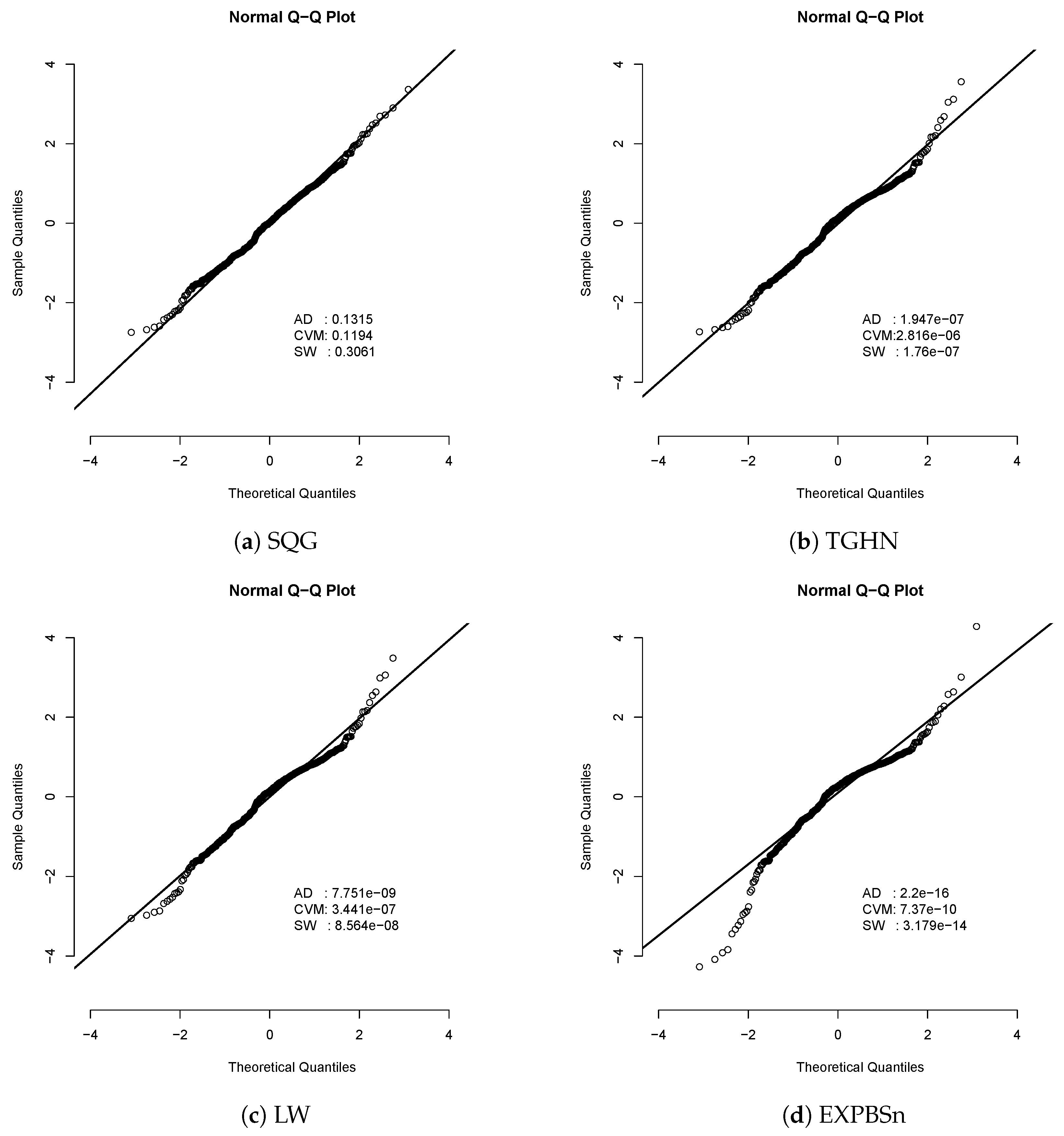
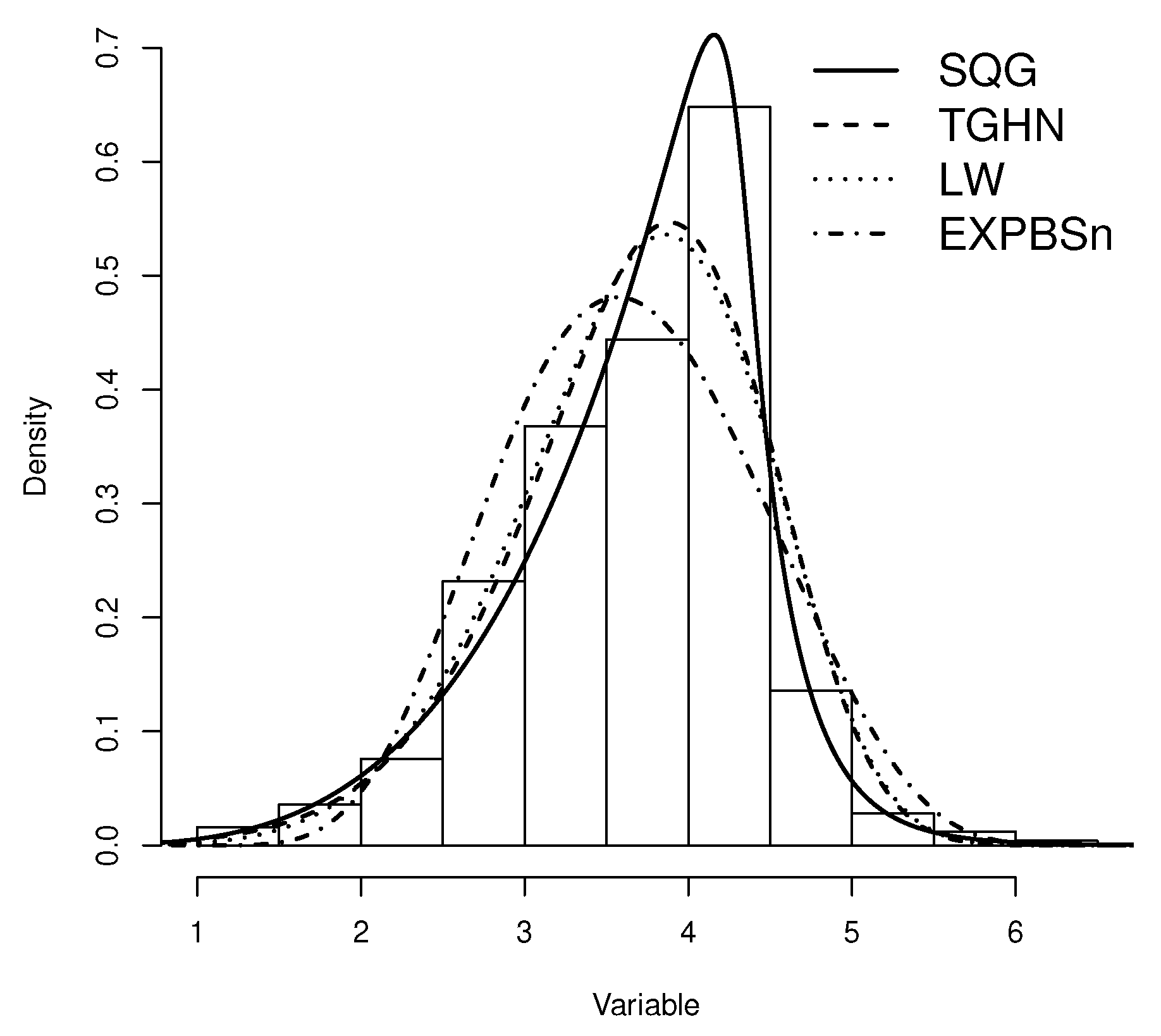
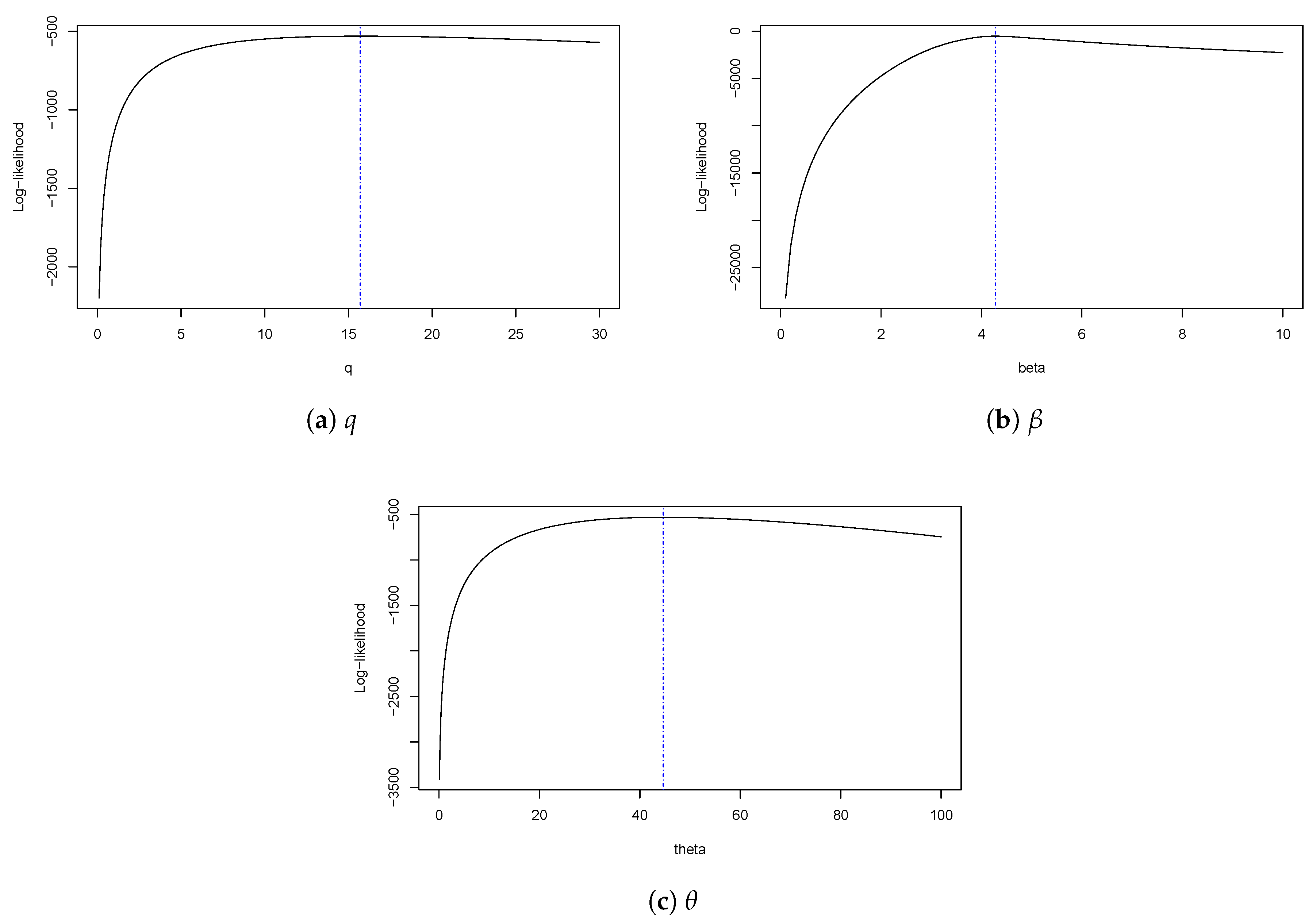
Table 5 presents ML estimates for the TGHN, LW, EXPBSn, and SQG distributions. For each model, the maximum value of the LLF, the corresponding values for the AIC and BIC criteria are also shown. It should be noted that both AIC and BIC show a better fit with the SQG model. Figure 7 shows plots of estimated densities for the models with the probability histogram and the profile log-likelihood function of q, , and in Figure 8. We note that the SQG density is closest to the frequency distribution of the data, this is because the SQG distribution is capable of modeling data with negative asymmetry. Finally, we have the qqplots for the quantile residual in the models and the p-values. Figure 9 shows that the SQG model fits better than the other models considered.
6. Discussion
In this article, we introduced a new three-parameter distribution called the SQG distribution. The new distribution is capable of modeling data that present different levels of asymmetry and high levels of kurtosis. It can be seen as an extension with one extra parameter of a particular case of the GENG distribution. This special case, which is finally extended, is not itself popular in the statistical literature. However, it corresponds to a distribution of two parameters (scale and shape) whose density function has particular concavity characteristics. The parameters of the proposed distribution were identified as parameters of scale, shape, and kurtosis, respectively, therefore this distribution did not present identifiability problems. We derived distributional moments, which allowed us to appropriately describe the asymmetry and kurtosis characteristics of the distribution. ML estimators were considered and numerical procedures were required for solving the likelihood equations. For ML estimates, the observed information matrix was used for estimating SE. We applied the proposed model to two real data set and the results demonstrated that the proposed model is very useful and flexible for non-negative data.
Author Contributions
All of the authors contributed significantly to this research article. Methodolgy, Y.A.I., H.V. and H.W.G.; software, H.J.G.; validation, H.J.G. All authors have read and agreed to the published version of the manuscript.
Funding
Y.A. Iriarte, H. Varela, and H.W. Gómez were supported by Grant SEMILLERO UA-2020 (Chile).
Conflicts of Interest
The authors declare no conflict of interest.
References
- Meeker, W.; Escobar, L. Statistical Methods for Reliability Data; Wiley: New York, NY, USA, 1998. [Google Scholar]
- Kleiber, C.; Kotz, S. Statistical Size Distributions in Economics and Actuarial Sciences; Wiley-Interscience: Hoboken, NJ, USA, 2003; ISBN 0-471-15064-9. [Google Scholar]
- Gómez, H.W.; Quintana, F.A.; Torres, F.J. A new family of slash-distribution with elliptical contours. Stat. Probab. Lett. 2008, 77, 717–725. [Google Scholar] [CrossRef]
- Arslan, O. An alternative multivariate skew-slash distribution. Stat. Probab. Lett. 2008, 78, 2756–2761. [Google Scholar] [CrossRef]
- Gómez, H.W.; Olivares-Pacheco, J.F.; Venegas, O. An extension of the generalized Birnbaum–Saunders distribution. Stat. Probab. Lett. 2009, 79, 331–338. [Google Scholar] [CrossRef]
- Olivares-Pacheco, J.F.; Cornide, H.; Monasterio, M. An extension of the two-parameter weibull distribution. Colomb. J. Stat. 2010, 33, 219–231. [Google Scholar]
- Olmos, N.M.; Varela, H.; Gómez, H.W.; Bolfarine, H. An extension of the half-normal distribution. Stat. Pap. 2012, 53, 875–886. [Google Scholar] [CrossRef]
- Olmos, N.M.; Varela, H.; Bolfarine, H.; Gómez, H.W. An extension of the generalized half-normal distribution. Stat. Pap. 2014, 55, 967–981. [Google Scholar] [CrossRef]
- Iriarte, Y.A.; Gómez, H.W.; Varela, H.; Bolfarine, H. Slashed Rayleigh distribution. Colomb. J. Stat. 2015, 38, 31–44. [Google Scholar] [CrossRef]
- Iriarte, Y.A.; Vilca, F.; Varela, H.; Gómez, H.W. Slashed Generalized Rayleigh distribution. Commun. Stat. Theory Methods 2017, 46, 4686–4699. [Google Scholar] [CrossRef]
- Reyes, J.; Barranco-Chamorro, I.; Gallardo, D.I.; Gómez, H.W. Generalized Modified Slash Birnbaum–Saunders Distribution. Symmetry 2018, 10, 724. [Google Scholar] [CrossRef] [Green Version]
- Casella, G.; Berger, R.L. Statistical Inference; Duxbury: Pacific Grove, CA, USA, 2002. [Google Scholar]
- R Core Team, R. A Language and Environment for Statistical Computing; R Foundation for Statistical Computing: Vienna, Austria, 2019; Available online: http://www.R-project.org/ (accessed on 4 March 2020).
- Andrews, D.F.; Herzberg, A.M. Data: A Collection of Problems from Many Fields for the Student and Research Worker; Springer Series in Statistics; Springer: New York, NY, USA, 1985. [Google Scholar]
- Barlow, R.E.; Toland, R.H.; Freeman, T. A Bayesian Analysis of Stress-Rupture Life of Kevlar 49/Epoxy Spherical Pressure Vessels. In Proceedings of the Canadian Conference in Application of Statistics; Marcel Dekker: New York, NY, USA, 1984. [Google Scholar]
- Salinas, H.; Iriarte, Y.; Astorga, J. A transmuted version of the generalized half-normal distribution. Proyecciones (Antofagasta) 2019, 38, 567–583. [Google Scholar] [CrossRef] [Green Version]
- Reyes, J.; Iriarte, Y.; Jodrá, P.; Gómez, H.W. The Slash Lindley-Weibull Distribution. Methodol. Comput. Appl. Probab. 2019, 21, 235–251. [Google Scholar] [CrossRef]
- Martínez-Flórez, G.; Bolfarine, H.; Gómez, H.W. An alpha-power extension for the Birnbaum–Saunders distribution. Statistics 2014, 48, 896–912. [Google Scholar] [CrossRef]
- Akaike, H. A new look at the statistical model identification. IEEE Trans. Autom. Control 1974, 19, 716–723. [Google Scholar] [CrossRef]
- Schwarz, G. Estimating the dimension of a model. Ann. Stat. 1978, 6, 461–464. [Google Scholar] [CrossRef]
- Dunn, P.; Smyth, G. Randomized Quantile Residual. J. Comput. Graph. Stat. 1996, 5, 236–244. [Google Scholar]
Figure 1.
Curves of the density function of the generalized gamma distribution (GENG) distribution for , and different values of .
Figure 1.
Curves of the density function of the generalized gamma distribution (GENG) distribution for , and different values of .

Figure 2.
Plot of pdf for a slashed quasi-gamma (SQG) distribution.

Figure 3.
Plots of the asymmetry and kurtosis coefficients for the SQG distribution.
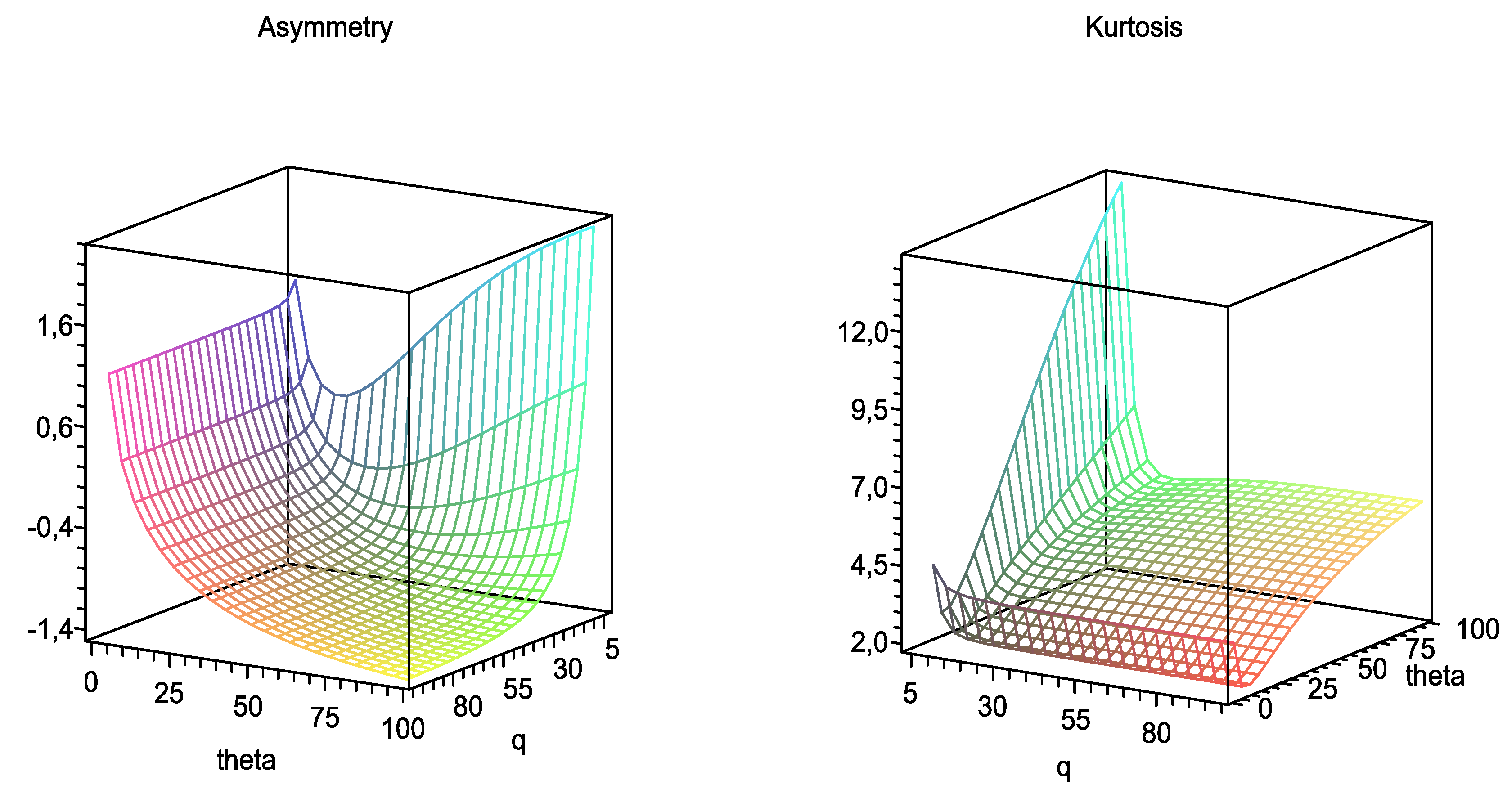
Figure 4.
SQG Model fitted by ML method for stress-rupture data set.

Figure 5.
Log-likelihood profile function for SQG distribution.
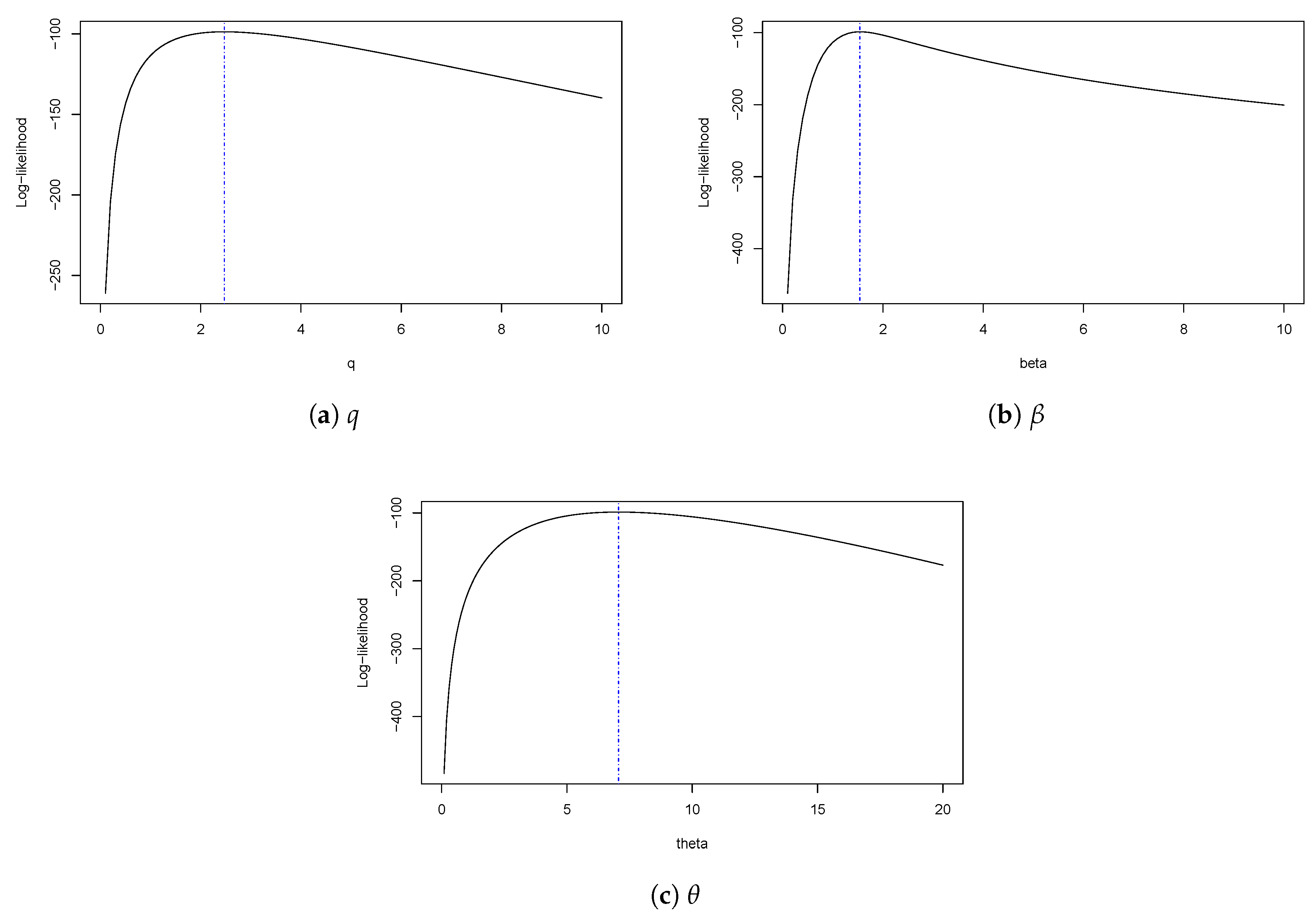
Figure 6.
Residual quantile for the fitted models to life of fatigue fracture data set. The p-values for the Anderson–Darling (AD), Cramer–Von Mises (CVM), and Shapiro–Wilk (SW) normality tests are also presented to check if the residual quantile came from the standard normal distribution. At a 5% significance level, for the three normality tests for the residual quantile, results suggest that the SQG model is appropriate for this data set while the rest of the models are not.
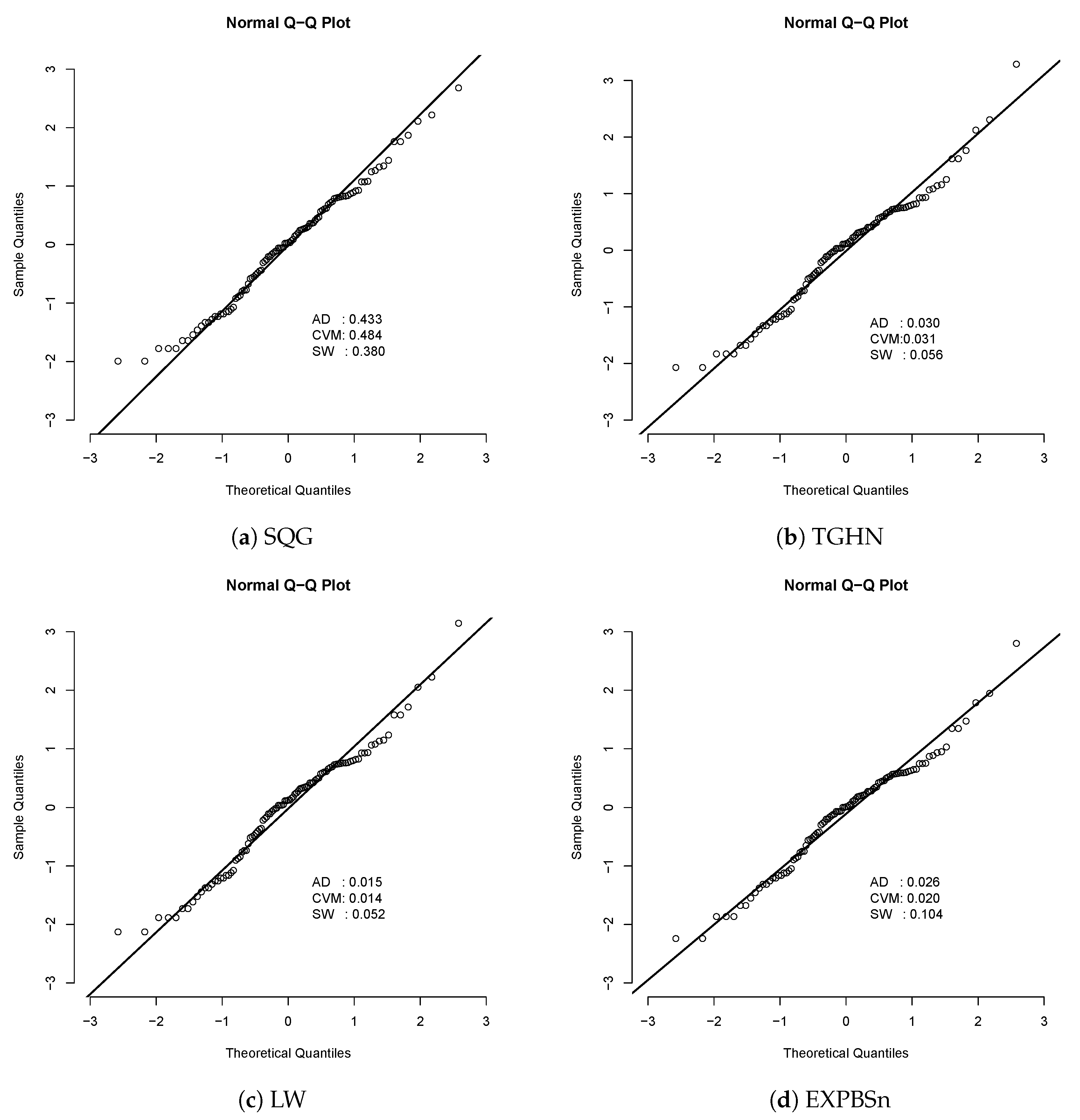
Figure 7.
SQG model fitted by the ML method for the logarithm of concentration.

Figure 8.
Log-likelihood profile function for SQG distribution.

Figure 9.
Residual quantile for the fitted models in the concentration of the data set. The p-values for the AD, CVM, and SW normality tests are also presented to check if the residual quantile came from the standard normal distribution. At a 5% significance level, for the three normality tests for the residual quantile, results suggest that the SQG model is appropriate for this data set while the rest of the models are not.

Table 1.
Maximum likelihood (ML) estimates for parameters , , and q of the SQG distribution.
| True Value | |||||
|---|---|---|---|---|---|
| 3 | 5 | 1 | 3.346(1.427) | 5.201(0.939) | 1.191(0.513) |
| 2 | 3.105(0.898) | 5.263(0.904) | 2.356(1.126) | ||
| 3 | 2.909(0.712) | 5.248(0.867) | 3.303(1.212) | ||
| 5 | 7 | 1 | 5.363(1.842) | 7.380(1.572) | 1.136(0.477) |
| 2 | 5.140(1.204) | 7.246(1.115) | 2.356(1.006) | ||
| 3 | 4.976(1.026) | 7.271(1.060) | 3.368(1.477) | ||
| 10 | 10 | 1 | 10.475(2.780) | 10.593(2.430) | 1.083(0.293) |
| 2 | 10.190(1.965) | 10.626(2.052) | 2.318(0.949) | ||
| 3 | 10.016(1.637) | 10.539(1.997) | 3.418(1.307) | ||
| True Value | |||||
| 3 | 5 | 1 | 3.050(0.829) | 5.141(0.660) | 1.053(0.238) |
| 2 | 3.087(0.654) | 5.087(0.581) | 2.262(0.773) | ||
| 3 | 3.062(0.573) | 5.110(0.599) | 3.223(1.058) | ||
| 5 | 7 | 1 | 5.099(1.100) | 7.238(1.038) | 1.034(0.195) |
| 2 | 5.080(0.837) | 7.169(0.907) | 2.167(0.587) | ||
| 3 | 5.088(0.761) | 7.166(0.844) | 3.210(1.122) | ||
| 10 | 10 | 1 | 10.173(1.859) | 10.376(1.697) | 1.041(0.169) |
| 2 | 10.187(1.422) | 10.165(1.355) | 2.153(0.530) | ||
| 3 | 10.141(1.201) | 10.200(1.231) | 3.369(1.007) | ||
| True Value | |||||
| 3 | 5 | 1 | 3.017(0.588) | 5.069(0.469) | 1.038(0.156) |
| 2 | 3.061(0.449) | 5.038(0.409) | 2.143(0.482) | ||
| 3 | 3.050(0.401) | 5.035(0.395) | 3.017(1.019) | ||
| 5 | 7 | 1 | 5.078(0.786) | 7.039(0.677) | 1.024(0.132) |
| 2 | 5.032(0.557) | 7.065(0.582) | 2.073(0.349) | ||
| 3 | 5.075(0.516) | 7.014(0.537) | 3.178(0.891) | ||
| 10 | 10 | 1 | 10.050(1.215) | 10.207(1.081) | 1.017(0.108) |
| 2 | 10.077(0.928) | 10.057(0.897) | 2.053(0.298) | ||
| 3 | 10.064(0.794) | 10.124(0.884) | 3.148(0.569) | ||
Table 2.
Descriptive statistics of the rupture stress times data set.
| Dataset | n | ||||
|---|---|---|---|---|---|
| Rupture stress times | 101 |
Table 3.
ML estimates with their respective standard errors (SE) for fitting models to the data set.
Table 3.
ML estimates with their respective standard errors (SE) for fitting models to the data set.
| Estimated | TGHN | LW | EXPBSn | SQG |
|---|---|---|---|---|
| - | 0.622 (1.021) | 3.420 (0.666) | 1.541 (0.170) | |
| - | 0.837 (0.109) | - | 7.063 (0.771) | |
| q | - | - | - | 2.471 (0.535) |
| 2.094 (0.330) | - | - | - | |
| 0.811 (0.064) | 1.046 (1.168) | 0.055 (0.025) | - | |
| 0.854 (0.168) | - | 3.661 (0.697) | - | |
| LLF | −102.277 | −102.597 | −100.692 | −98.669 |
| AIC | 210.554 | 211.195 | 207.385 | 203.338 |
| BIC | 218.399 | 219.040 | 215.230 | 211.183 |
Table 4.
Descriptive statistics of the logarithm of the concentration data set.
| Dataset | n | ||||
|---|---|---|---|---|---|
| Logarithm of the | 500 |
Table 5.
ML estimates with its respective SE for fitting models to the data set.
| Estimated | TGHN | LW | EXPBSn | SQG |
|---|---|---|---|---|
| - | 9.646 (3.752) | 0.060 (0.010) | 4.281 (0.036) | |
| - | 5.723 (0.195) | - | 44.664 (2.214) | |
| q | - | - | - | 15.710 (1.586) |
| 3.738 (0.053) | - | - | - | |
| 3.120 (0.163) | 157.002 (345.840) | 5.199 (0.110) | - | |
| −0.892 (0.082) | - | 0.033 (0.012) | - | |
| LLF | −555.785 | −557.436 | −591.954 | −530.462 |
| AIC | 1117.571 | 1120.872 | 1189.908 | 1066.924 |
| BIC | 1130.215 | 1133.516 | 1202.552 | 1079.568 |
© 2020 by the authors. Licensee MDPI, Basel, Switzerland. This article is an open access article distributed under the terms and conditions of the Creative Commons Attribution (CC BY) license (http://creativecommons.org/licenses/by/4.0/).
Share and Cite
MDPI and ACS Style
Iriarte, Y.A.; Varela, H.; Gómez, H.J.; Gómez, H.W. A Gamma-Type Distribution with Applications. Symmetry 2020, 12, 870. https://doi.org/10.3390/sym12050870
AMA Style
Iriarte YA, Varela H, Gómez HJ, Gómez HW. A Gamma-Type Distribution with Applications. Symmetry. 2020; 12(5):870. https://doi.org/10.3390/sym12050870
Chicago/Turabian StyleIriarte, Yuri A., Héctor Varela, Héctor J. Gómez, and Héctor W. Gómez. 2020. "A Gamma-Type Distribution with Applications" Symmetry 12, no. 5: 870. https://doi.org/10.3390/sym12050870
Note that from the first issue of 2016, this journal uses article numbers instead of page numbers. See further details here.