Approximating the Distribution of the Product of Two Normally Distributed Random Variables

Abstract

The distribution of the product of two normally distributed random variables has been an open problem from the early years in the XXth century. First approaches tried to determinate the mathematical and statistical properties of the distribution of such a product using different types of functions. Recently, an improvement in computational techniques has performed new approaches for calculating related integrals by using numerical integration. Another approach is to adopt any other distribution to approximate the probability density function of this product. The skew-normal distribution is a generalization of the normal distribution which considers skewness making it flexible. In this work, we approximate the distribution of the product of two normally distributed random variables using a type of skew-normal distribution. The influence of the parameters of the two normal distributions on the approximation is explored. When one of the normally distributed variables has an inverse coefficient of variation greater than one, our approximation performs better than when both normally distributed variables have inverse coefficients of variation less than one. A graphical analysis visually shows the superiority of our approach in relation to other approaches proposed in the literature on the topic.

1. Introduction

The first approach for finding the distribution of the product of two random variables with normal distribution was based on the product of two standard normal distributed random variables. In this case, Bessel type functions were used to approximate such a product [1]. Moments of the distributions of powers and products of normally distributed variables were studied in [2]. Other approaches presented in [3,4] considered a Pearson type function. In [5], there are several advances regarding the distribution of the product of two normally distributed random variables, but some of these advances need integrals that do not have an analytical solution and neither are defined at zero; see also [6]. A number of authors [7,8,9,10,11] employed the improvement of the computational methods to provide approximate numerical solutions for the mentioned integrals. Other alternative approaches are very limited. For example, the Bessel function method proposed in [9] presents a good approximation, but only for the product of two standard normal distributions and, moreover, it is not defined at zero. In [12,13,14,15], other approaches are presented, including Stein’s operators and distributional theory. Another approach is to use any other distribution to approximate the probability density function (PDF) of the mentioned product. For example, in [16], the Gram-Charlier series are utilized to approximate a distribution while using the cumulative function distribution (CDF) of another distribution. The moment-generating function (MGF) of the product of two normally distributed variables, as reported in [1,17], can be used to calculate its coefficients of skewness and kurtosis. The values of these coefficients of the product of two normally distributed random variables do not coincide with the corresponding values of the normal distribution, that is, coefficient of skewness equal to zero and coefficient of kurtosis equal to three (or zero, when the excess of kurtosis is considered). Some efforts to find the distribution of the product of two random variables with asymmetric (skew) distributions of bounded-support, such as beta and gamma, have been conducted in [13,18]. However, to the best of our knowledge, until now the determination of the distribution of the product of two normally distributed random variables continues being an open problem.

The skew-normal (SN) distribution, introduced in [19], is a generalization of the normal distribution in order to consider the existence of skewness, allowing for the modeling of data with skew distributions [20,21,22]. In recent developments, some authors [23,24,25,26,27] performed new generalizations of the SN distribution. One of them is known like the extended skew-normal (ESN) distribution, which is parameterized in terms of its location, scale, shape, and truncation. The ESN distribution permits the modeling of data with different degrees of skewness and kurtosis by means of its shape and truncation parameters. To the best of our knowledge, until now SN type distributions have not been considered to approximate the distribution of the product of two normally distributed variables.

The objective of this paper is to approximate the distribution of the product of two normally distributed random variables by using the ESN distribution. This new approach has two stages: (i) the first of them is the determination of values for the shape and truncation parameters of the ESN distribution related to the skewness and kurtosis values of the product; and, (ii) the second stage is the determination of the values for the other two parameters (location and scale), using the mean and variance of the product. Although good approximations for the mean and variance of the product of two normally distributed random variables have been proposed, unfortunately, no good approximations for its skewness and kurtosis have been obtained. We explore different degrees of skewness and kurtosis in order to evaluate our approximation. When one of the normally distributed variables has an inverse coefficient of variation greater than one, our approximation performs better than when both normally distributed variables have inverse coefficients of variation less than one. However, in general, the superiority of this new approach in relation to other approaches proposed in the literature on such topic is evident.

The rest of the paper is organized as follows. In Section 2, the moments of the distribution of the product of two normally distributed random variables are introduced. Section 3 provides some characteristics of the ESN distribution. In Section 4, we focus on the approximation of the distribution of the product of two normally distributed random variables through the ESN distribution. Finally, Section 5 is devoted to some conclusions, discussion, and ideas for further investigation. The computational codes used in this paper are available upon request to the authors.

2. Product of Two Normal Random Variables

Let $X\sim \mathrm{N}({\mu }_X,{\sigma }_X)$ and $Y\sim \mathrm{N}({\mu }_Y,{\sigma }_Y)$ be two normally distributed random variables with correlation coefficient $\mathrm{Corr}(X,Y)=\rho \in [-1,1]$. Subsequently, the MGF of $U=XY$ is given by

$$\begin{array}{cc}\hfill M_U\left(t\right)& =\frac{1}{2\pi }{\int }_{-\infty }^{\infty }{\int }_{-\infty }^{\infty }exp\left(-\frac{{(x-{\mu }_X)}^2}{2{\sigma }_X^2}-\frac{{(y-{\mu }_Y)}^2}{2{\sigma }_Y^2}\right)exp\left(xyt\right)\mathrm{d}x\mathrm{d}y\hfill \\ & =\frac{1}{{(1-{\sigma }_X^2{\sigma }_Y^2{t}^2)}^{1/2}}exp\left(\frac{({\sigma }_X^2{\mu }_Y^2+{\sigma }_Y^2{\mu }_X^2)t^2+2{\mu }_X{\mu }_{Y}t}{2(1-{\sigma }_X^2{\sigma }_Y^2{t}^2)}\right).\hfill \end{array}$$

(1)

Note that expression defined in (1) can be formulated in terms of the inverse coefficients of variation of X and Y established by ${\delta }_X={\mu }_X/{\sigma }_X$ and ${\delta }_Y={\mu }_Y/{\sigma }_Y$, which are considered to be small when its value is less than one. Thus, from (1) and based on $\rho$, ${\delta }_X$ and ${\delta }_Y$, we have that:

• Mean: $\mathrm{E}\left(U\right)={\delta }_X{\delta }_Y+\rho$.
• Variance: $\mathrm{Var}\left(U\right)=1+{\rho }^2+2\rho {\delta }_X{\delta }_Y+{\delta }_X^2+{\delta }_Y^2$.
• Coefficient of variation: $\mathrm{CV}\left(U\right)={\displaystyle \frac{\sqrt{1+{\rho }^2+2\rho {\delta }_X{\delta }_Y+{\delta }_X^2+{\delta }_Y^2}}{{\delta }_X{\delta }_Y+\rho }}$.
• Coefficient of skewness: $\mathrm{CS}\left(U\right)={\displaystyle \frac{2({\rho }^3+3{\delta }_X{\delta }_Y+3{\rho }^2{\delta }_X{\delta }_Y+3\rho (1+{\delta }_X^2+{\delta }_Y^2))}{{(1+{\rho }^2+{\delta }_X^2+{\delta }_Y^2+2\rho {\delta }_X{\delta }_Y)}^{3/2}}}$.
• Excess of kurtosis: $\mathrm{EK}\left(U\right)={\displaystyle \frac{6(1+{\rho }^4+2{\delta }_X^2+12\rho {\delta }_X{\delta }_Y+4{\rho }^3{\delta }_X{\delta }_Y+2{\delta }_Y^2+6{\rho }^2(1+{\delta }_X^2+{\delta }_Y^2))}{{(1+{\rho }^2+{\delta }_X^2+{\delta }_Y^2+2\rho {\delta }_X{\delta }_Y)}^2}}.$
• Skewness/kurtosis ratio:

  $$\mathrm{SKR}\left(U\right)=\frac{\sqrt{1+{\delta }_X^2+{\delta }_Y^2+2{\delta }_X{\delta }_Y\rho +{\rho }^2}\left(3{\delta }_X{\delta }_Y+3(1+{\delta }_X^2+{\delta }_Y^2)\rho +3{\delta }_X{\delta }_Y{\rho }^2+{\rho }^3\right)}{3\left(1+2{\delta }_Y^2+6(1+{\delta }_Y^2){\rho }^2+{\rho }^4+4{\delta }_X{\delta }_Y\rho (3+{\rho }^2)+{\delta }_X^2(2+6{\rho }^2)\right)}.$$

  (2)

From (2), note that the skewness/kurtosis ratio of the product of two normally distributed random variables is composed by three factors. By assuming $\rho \in [-1,1]$ and ${\delta }_X,{\delta }_Y\in [-1,1]$, the ranges for these factors are analyzed as follows:

(i)

First factor $\sqrt{1+{\delta }_X^2+{\delta }_Y^2+2{\delta }_X{\delta }_Y\rho +{\rho }^2}$: its minimum value is one, which is reached at $\rho ={\delta }_X={\delta }_Y=0$, while its maximum value is $\sqrt{6}$ and reached at $\rho =1,{\delta }_X={\delta }_Y=-1$. Afterwards, the first factor ranges between $[1,\sqrt{6}]$.

(ii)

Second factor $\left(3{\delta }_X{\delta }_Y+3(1+{\delta }_X^2+{\delta }_Y^2)\rho +3{\delta }_X{\delta }_Y{\rho }^2+{\rho }^3\right)$: its minimum value is $-16$ and reached when $\rho =-1,{\delta }_X=-1,{\delta }_Y=1$, while its maximum is 16 at $\rho =1,{\delta }_X=-1,{\delta }_Y=-1$. Thus, the second factor ranges between $[-16,16]$.

(iii)

Third factor $3(1+2{\delta }_Y^2+6(1+{\delta }_Y^2){\rho }^2+{\rho }^4+4{\delta }_X{\delta }_Y\rho (3+{\rho }^2)+{\delta }_X^2(2+6{\rho }^2))$: its minimum value is three and reached at $\rho ={\delta }_X={\delta }_Y=0$, while its maximum value is 120 at $\rho =1,{\delta }_X={\delta }_Y=-1$. Hence, the denominator of this skewness/kurtosis ratio is in the range $[3,120]$.

Therefore, one can deduce that the skewness/kurtosis ratio of the product of two normally distributed random variables is in the range $[-0.38,0.38]$.

In [28,29], the authors analyzed the coefficients of skewness and kurtosis of the product of two normally distributed random variables, according to different values of parameters of the two normal distributions.

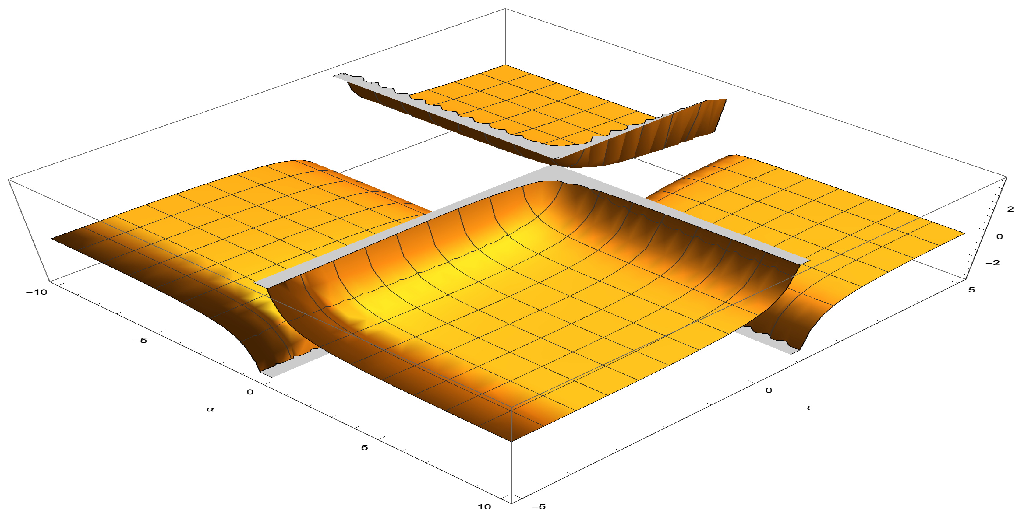
The skewness/kurtosis ratio of the product of two normally distributed random variables is explored and depicted in Figure 1. From this figure, note that the influence of the correlation on the shape of the ratio is limited. However, the inverse coefficient of variation has an important effect on this ratio. There is a saddle-point at $(0,0)$ and, when the signs of ${\delta }_X$ and ${\delta }_Y$ are the same, the ratio tends to a maximum, whereas, for different signs, the ratio tends to a minimum. Figure 2 displays the scenario for small values of the inverse coefficient of variation, which is less than one in absolute value for the two normally distributed variables.

3. The Extended Skew-Normal Distribution

Now, let X be a random variable with SN distribution of location parameter $\xi$, scale parameter $\omega$ and skewness parameter $\alpha$, which is denoted by $X\sim \mathrm{SN}(\xi ,\omega ,\alpha )$; for more details of the SN distribution, see [25]. Subsequently, the PDF of X is given by

$$f_X\left(x\right)=\frac{2}{\omega }\varphi \left(\frac{x-\xi }{\omega }\right)\mathsf{\Phi }\left(\alpha \left(\frac{x-\xi }{\omega }\right)\right),x\in \mathbb{R},\xi \in \mathbb{R},\omega \in {\mathbb{R}}^{+},\alpha \in \mathbb{R},$$

(3)

where $\varphi$ and $\mathsf{\Phi }$ are the standard normal PDF and CDF, respectively. Note that, if $\alpha =0$, then the PDF of X defined in (3) reduces to the normal PDF. The SN distribution has interesting properties, some of which are used in this paper and presented next. If $X\sim \mathrm{SN}(\xi ,\omega ,\alpha )$, then:

• Mean: $\mathrm{E}\left(X\right)=\xi +\omega \sqrt{{\displaystyle \frac{2{\alpha }^2}{\pi (1+{\alpha }^2)}}}$;
• Variance: $\mathrm{Var}\left(X\right)=\omega \left(1-{\displaystyle \frac{2{\alpha }^2}{\pi (1+{\alpha }^2)}}\right)$.

As mentioned, the ESN distribution is an extension of the SN distribution, as indicated below; for more details of the ESN distribution, see [25]. In this case, the notation $Y\sim \mathrm{ESN}(\xi ,\omega ,\alpha ,\tau )$ is employed, where $\xi ,\omega ,\alpha$ and $\tau$ are location, scale, shape, and truncation parameters, respectively. The PDF of $Y\sim \mathrm{ESN}(\xi ,\omega ,\alpha ,\tau )$ is expressed as

$$f_Y\left(y\right)=\frac{1}{\omega }\varphi \left(\frac{y-\xi }{\omega }\right)\frac{\mathsf{\Phi }\left(\tau \sqrt{{\alpha }^2+1}+\frac{\alpha (y-\xi )}{\omega }\right)}{\mathsf{\Phi }\left(\tau \right)},y\in \mathbb{R},\xi \in \mathbb{R},\omega \in {\mathbb{R}}^{+},\alpha \in \mathbb{R},\tau \in \mathbb{R}.$$

Note that, if $\tau =0$, the SN PDF defined in (3) is obtained and when $\tau =\alpha =0$, the normal distribution is get. The standard ESN distribution is a particular case of the ESN distribution with parameters $\xi =0$ and $\omega =1$. In addition, observe that the shape of the ESN PDF is very similar to the normal PDF (with different levels of skewness) when $\tau >0$. For negative values of $\tau$, several types of shapes are obtained. When $\alpha$ is large (for example, for $\left|\alpha \right|>50)$, the ESN PDF is concentrated around the mean, the variance is small, and the sign of the coefficient of skewness is determined by the sign of $\alpha$. Statistics as the mean, variance, and coefficients of skewness and kurtosis of the ESN distribution can be calculated from its MGF after taking derivatives. Subsequently, following [25], the ESN MGF may be computed from the expression $Y=\xi +\omega Z$, where $Z\sim \mathrm{ESN}(0,1,\alpha ,\tau )$, as 

$$M_Y\left(t\right)=exp\left(\xi t+\frac{{\omega }^2{t}^2}{2}\right)\frac{\mathsf{\Phi }\left(\tau +\frac{\alpha \omega t}{\sqrt{1+{\alpha }^2}}\right)}{\mathsf{\Phi }\left(\tau \right)}.$$

(4)

Hence, from (4), the following expressions are obtained:

• Mean: $\mathrm{E}\left(Y\right)=\xi +{\displaystyle \frac{exp(-{\tau }^2/2)\alpha \omega \sqrt{2/\pi }}{2\mathsf{\Phi }\left(\tau \right)\sqrt{1+{\alpha }^2}}}.$
• Variance: $\mathrm{Var}\left(Y\right)={\omega }^2\left(1-{\displaystyle \frac{exp(-{\tau }^2){\alpha }^2\left(2+exp\left({\tau }^2/2\right)2\tau \mathsf{\Phi }\left(\tau \right)\sqrt{2\pi }\right)}{\pi (1+{\alpha }^2){\left(2\mathsf{\Phi }\left(\tau \right)\right)}^2}}\right).$
• Coefficient of variation: $\mathrm{CV}\left(Y\right)={\displaystyle \frac{\sqrt{{\omega }^2\left(1-\frac{exp(-{\tau }^2){\alpha }^2\left(2+exp\left({\tau }^2/2\right)2\tau \mathsf{\Phi }\left(\tau \right)\sqrt{2\pi }\right)}{\pi \left(1+{\alpha }^2\right){\left(2\mathsf{\Phi }\left(\tau \right)\right)}^2}\right)}}{\xi +\frac{exp(-{\tau }^2/2)\alpha \omega \sqrt{2/\pi }}{2\mathsf{\Phi }\left(\tau \right)\sqrt{1+{\alpha }^2}}}}.$
• Coefficient of skewness:

  $$\mathrm{CS}\left(Y\right)=\frac{exp\left(-\frac{3{\tau }^2}{2}\right){\alpha }^3\left(4\sqrt{\frac{2}{\pi }}+6exp\left(\frac{{\tau }^2}{2}\right)2\tau \mathsf{\Phi }\left(\tau \right)+exp\left(t^2\right)\sqrt{2\pi }\left({\tau }^2-1\right){\left(2\mathsf{\Phi }\left(\tau \right)\right)}^2\right)}{\pi {(1+{\alpha }^2)}^{\frac{3}{2}}{\left(2\mathsf{\Phi }\left(\tau \right)\right)}^3{\left(1-\frac{exp\left(-{\tau }^2\right){\alpha }^2\left(2+exp\left(\frac{{\tau }^2}{2}\right)\sqrt{2\pi }2\tau \mathsf{\Phi }\left(\tau \right)\right)}{\pi \left(1+{\alpha }^2\right){\left(2\mathsf{\Phi }\left(\tau \right)\right)}^2}\right)}^{3/2}}.$$
• Excess of kurtosis:

  $$\mathrm{EK}\left(Y\right)=\frac{exp\left(-2{\tau }^2\right){\alpha }^4\left(-24-24exp\left(\frac{{\tau }^2}{2}\right)\sqrt{2\pi }2\tau \mathsf{\Phi }\left(\tau \right)-2exp\left(t^2\right)\pi \left(7{\tau }^2-4\right){\left(2\mathsf{\Phi }\left(\tau \right)\right)}^2+\sqrt{2}exp\left(\frac{3t^2}{2}\right){\pi }^{\frac{3}{2}}\tau \left({\tau }^2-3\right){(2\mathsf{\Phi }\left(\tau \right)-2)}^3\right)}{{\pi }^2{(1+{\alpha }^2)}^2{\left(2\mathsf{\Phi }\left(\tau \right)\right)}^4{\left(-1+\frac{exp\left(-{\tau }^2\right){\alpha }^2\left(2+exp\left(\frac{{\tau }^2}{2}\right)\sqrt{2\pi }2\tau \mathsf{\Phi }\left(\tau \right)\right)}{\pi \left(1+{\alpha }^2\right){\left(2\mathsf{\Phi }\left(\tau \right)\right)}^2}\right)}^2}.$$
• Skewness/kurtosis ratio:

  $$\begin{array}{ccc}\mathrm{SKR}\left(Y\right)\hfill & =& \frac{exp({\tau }^2/2)\pi \sqrt{1+{\alpha }^2}\mathsf{\Phi }{\left(\tau \right)}^2\left(\sqrt{2/\pi }+3exp({\tau }^2/2)\tau +exp\left({\tau }^2\right)\sqrt{2\pi }({\tau }^2-1)\mathsf{\Phi }{\left(\tau \right)}^2\right)}{\left(-3+\sqrt{2}exp\left(\frac{3{\tau }^2}{2}\right){\pi }^{3/2}\tau ({\tau }^2-3){(\mathsf{\Phi }(-\tau )-1)}^3-6exp({\tau }^2/2)\sqrt{2\pi }\tau \mathsf{\Phi }\left(\tau \right)-exp\left({\tau }^2\right)\pi (7{\tau }^2-4)\mathsf{\Phi }{\left(\tau \right)}^2\right)}\hfill \\ & & \times \frac{1}{\alpha }\sqrt{1-\frac{exp(-{\tau }^2){\alpha }^2\left(1+exp({\tau }^2/2)\sqrt{2\pi }\tau \mathsf{\Phi }\left(\tau \right)\right)}{2\pi ({\alpha }^2+1)\mathsf{\Phi }{\left(\tau \right)}^2}}.\hfill \end{array}$$

  (5)

Note that the ESN skewness/kurtosis ratio given in (5) only depends on the parameters $\alpha ,\tau$ and on the standard normal CDF, Φ namely. Therefore, there is no influence of the two other parameters $\xi$ and $\omega$ on this ratio. The sign of $\alpha$ determines the sign of the skewness (positive or negative). If $\alpha$ is positive, the ratio moves from a positive value to a negative value, while for $\alpha <0$, the ratio goes from negative values to positive values. When $\alpha =0$, the ESN excess of kurtosis is zero and then its skewness/kurtosis ratio is not defined, but no problem exists for other values of $\alpha$. When $\tau =1$, there is a discontinuity in this ratio. For $\tau >1$, the ratio is always negative and, for  $\tau <1$, it is always positive. Notice that, with the values of skewness and kurtosis, it is possible to only calculate the values of two parameters ($\alpha ,\tau$), in whose case a numerical solution to the equations is needed, which is sensitive to the initial point. With the values of the mean and variance, the other two parameters, $\xi$ and $\omega$ namely, can be obtained.

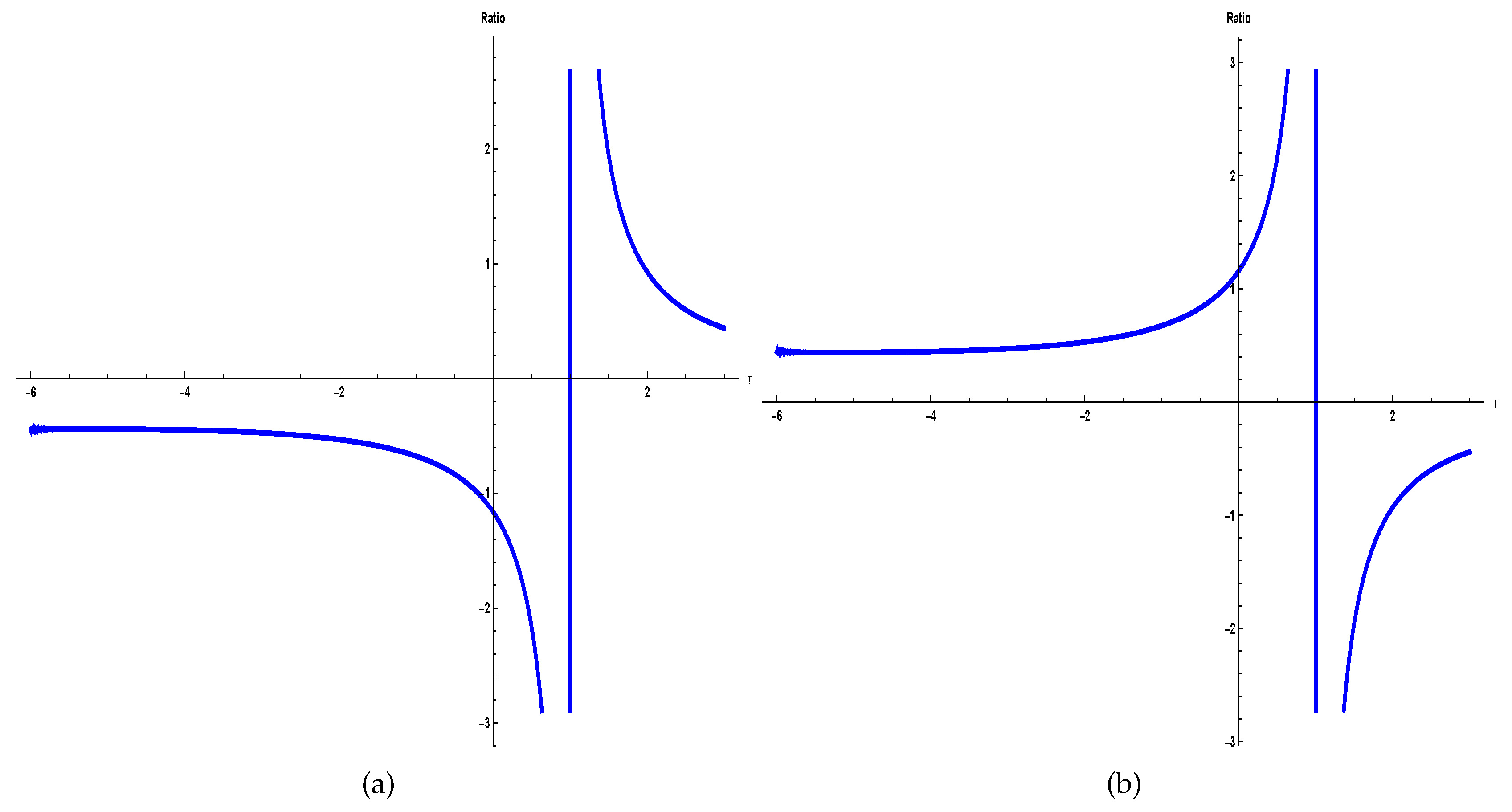
Next, the ESN skewness/kurtosis ratio is graphically analyzed according to different values of its parameters; see Figure 3. In this figure, the ESN skewness/kurtosis ratio is depicted as a function of the parameters $\alpha$ and $\tau$. The shape of this ratio is no smooth as in the case of the skewness/kurtosis ratio of the product of two normally distributed variables. The presence of gaps and changes on the direction of the shape of this ratio may be observed in this figure. The ratio is a non-continuous function with horizontal asymptotes at zero and $\pm 0.4$. Observe that the ESN skewness/kurtosis ratio is an increasing function of $\tau$; see Figure 4. When $\tau$ is positive, the ESN skewness/kurtosis ratio is small.

4. Approximation for the Product Distribution with ESN Distributions

An approximation for the distribution of the product of two normally distributed variables using the ESN distribution is considered next. By using the MGF of the product of two normally distributed variables, the values of the mean, variance, coefficient of skewness, and excess of kurtosis are obtained. Subsequently, an ESN distribution with the same values for these statistics is assumed. By employing (4), the values of the parameters $\xi ,\omega ,\alpha$, and $\tau$ for the corresponding ESN distribution are calculated.

The parameters $\alpha$ and $\tau$ of the ESN distribution must be obtained in order to determine the skewness and kurtosis of the product $U=XY$ as a function of ${\delta }_X,{\delta }_Y$ and $\rho$. In a first stage, a system of two equations must be solved in terms of $\alpha$ and $\tau$. Afterwards, in a second stage, to determine the ESN parameters $\omega$ and $\xi$, the other two equations for the mean and variance of the product must be solved. The solution must be reached using the values of parameters obtained in the previous stage. The following problems are associated with the first stage:

• As non-linear equations are generated, suitable numerical methods are required.
• As the solution obtained can be sensitive to the initial point, different points can be tested to avoid the stop at an inadequate point.
• Values of the coefficient of skewness and the excess of kurtosis are not always reached.

However, our approximation has the following advantages:

• A distribution is used considering a correlation $\rho \ne 0$ differently of other approaches [8,9], where only non-correlated variables ($\rho =0$) were considered.
• A known distribution is employed and its PDF for any value of the product can be calculated with no need of numerical integrals.
• Inference using the ESN distribution is available.

Monte Carlo simulations are utilized with ${10}^9$ replications of the product of two normally distributed variables while using a bivariate normal distribution with correlation $\rho$. Thus, the values of the mean, variance, skewness, and kurtosis are obtained according to the previously described procedure.

For this simulation, the R software was used [30]. Specifically, the sn package [31] was utilized, which provides functions for the SN and ESN PDFs and their cumulants. These cumulants are employed to derive the values of skewness and kurtosis.

The product of two normally distributed variables while using the bivariate normal distribution with correlation $\rho$ was obtained. Its mean, variance, skewness and kurtosis were calculated with the corresponding MGF. The BB package [32] was used, which contains the BBSolve function, in order to solve the system of equations described above.

Table 1. Statistics for the product of two normally distributed variables: X and Y with $\rho =0.5$ and ${\delta }_X,{\delta }_Y$ as listed.

Product	Mean	Variance	Skewness	Kurtosis
	${\delta }_X=0.5,{\delta }_Y=0.25$
Theoretical value	2.500	27.0000	2.3338	9.25995
Simulated value	2.499	26.9927	2.3337	9.40562
Approximate value	2.500	27.0000	1.9855	9.26592
	${\delta }_X=2.0,{\delta }_Y=2.5$
Theoretical value	0.5500	1.650	1.06679	1.5634
Simulated value	0.5499	1.649	1.06684	1.5645
Approximate value	0.5500	1.650	1.06677	1.5634
	${\delta }_X=0.5,{\delta }_Y=2.5$
Theoretical value	0.7000	1.4400	1.18981	2.479685
Simulated value	0.6999	1.4396	1.18956	2.479581
Approximate value	0.7000	1.4400	1.18981	2.479685

reports the values of the statistics of the product of two normally distributed variables $X\sim \mathrm{N}(1.0,2.0)$ and $Y\sim \mathrm{N}(0.5,2.0)$ with $\rho =0.5$, where the performance of the approximation, based on the ESN distribution, can be analyzed. The values are the same for the mean and variance, while a slight difference for the excess of kurtosis is detected. However, in the case of the skewness, the difference is large, being around $30\%$.

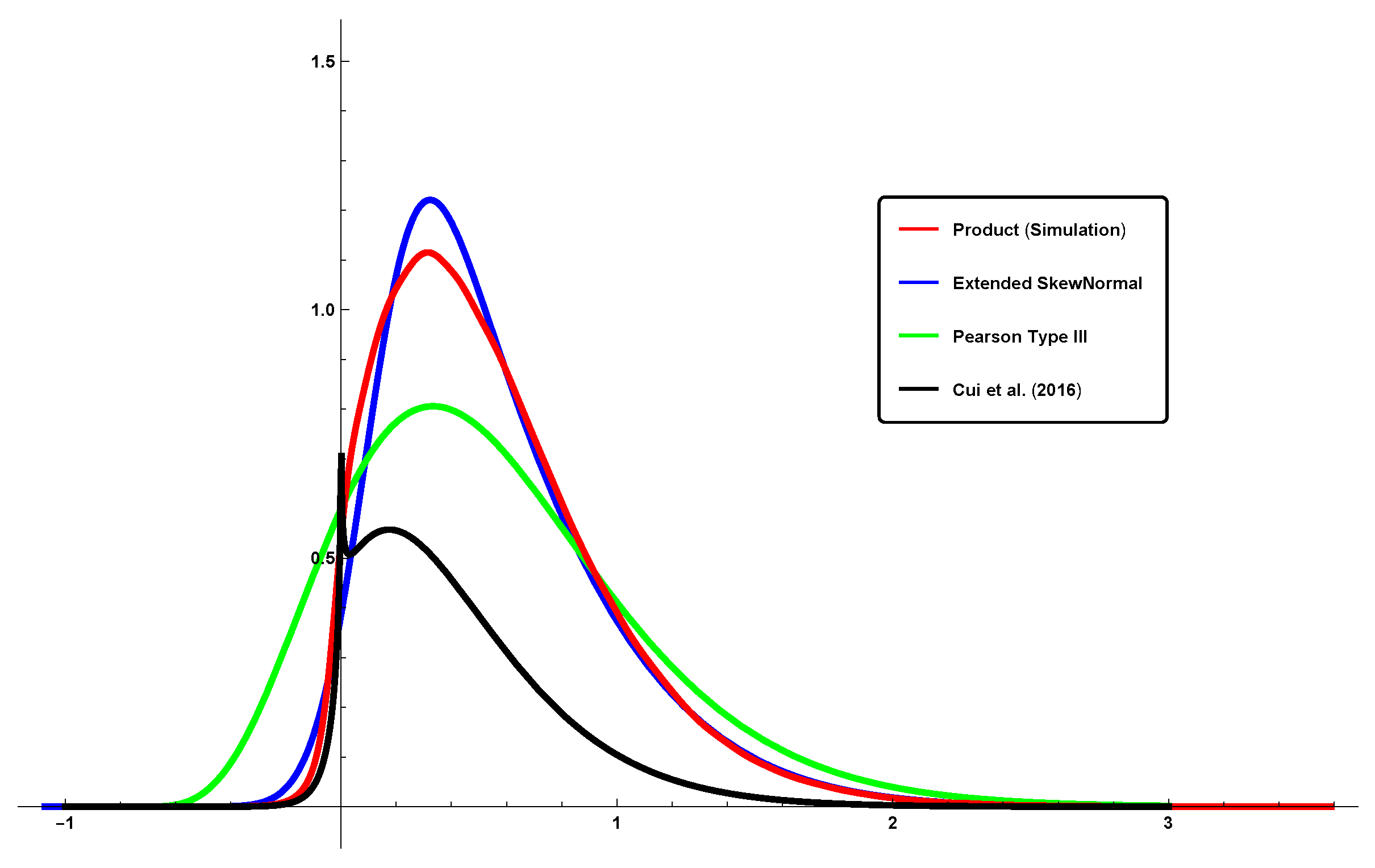
Figure 5 depicts the behavior of the approximation, where both inverse coefficients of variation are small (less than one), specifically, ${\delta }_X=0.5<1$ and ${\delta }_Y=0.25<1$. Now, consider the case of $X\sim \mathrm{N}(1.0,0.5)$ and $Y\sim \mathrm{N}(0.5,0.2)$, with $\rho =0.5$, ${\delta }_X=2.0>1$ and ${\delta }_Y=2.5>1$, that is, the two variables have a large value for their inverse coefficients of variation. The results are reported in Table 1, with a high similarity between the theoretical values and those simulated by the ESN distribution; see also Figure 6.

The approximation that is proposed in this paper is sensitive to the values of the inverse coefficients of variation of the normally distributed variables. For the scenarios considered, when the two inverse coefficients of variation are less than one, the approximation based on the ESN distribution does not work well. However, when the two inverse coefficients of variation are greater than one, the approximation based on the ESN distribution works very good. Moreover, in order to have a good performance, there is only the need that one of the inverse coefficients of variation is greater than one, as reported in Figure 7 and Table 1. Therefore, the inverse coefficients of variation of both normally distributed variables determine the performance of our approximation based on the ESN distribution. Observe that the expression of the ESN skewness/kurtosis ratio, defined in (5), is always less than 0.4 (in absolute value). Thus, the ESN skewness/kurtosis ratio is never equal to the ratio of skewness over kurtosis of the product of two normally distributed variables when ${\delta }_X,{\delta }_Y$ are in the range $[-1,1]$.

Note that other alternative approaches are very limited. For example, as mentioned, the approach that is based on the Bessel function method presents a good approximation, but only for the product of two standard normal distributions, and, moreover, it is not defined at zero. In Figure 5, Figure 6 and Figure 7, other approaches like Pearson type III distribution [3], or the function presented in [7] that we call the Cui et al. approach, are depicted as comparison with our approach. Observe that, clearly, the results are worse than those obtained with our ESN approach. Notice that the function provided in [7] does not converge and then it is not possible to represent it in Figure 5.

Notice that our approximation that is based on the ESN distribution works well for several examples of the product of two normally distributed variables, when ${\delta }_X$ or ${\delta }_Y$ are greater than one; see

Table 2. Comparison of statistics of the product of two normality distributed variables $X\sim \mathrm{N}({\mu }_X,{\sigma }_X)$ and $Y\sim \mathrm{N}({\mu }_Y,{\sigma }_Y)$ with indicated $\rho$ and ESN approximation statistics.

			Theoretical Value				Approximated Value
	${\mathit{\delta }}_{\mathit{X}}$	${\mathit{\delta }}_{\mathit{Y}}$	Mean	Variance	Skewness	Kurtosis	Mean	Variance	Skewness	Kurtosis
		$\rho =0.5$
$X\sim \mathrm{N}(2,1.75)$ $Y\sim \mathrm{N}(1,0.25)$	1.1	4.0	2.2188	4.4268	0.8043	1.0415	2.2188	4.4268	0.8043	1.0415
$X\sim \mathrm{N}(2,1.50)$ $Y\sim \mathrm{N}(1,0.50)$	1.3	2.0	2.3750	5.4531	1.3445	2.5612	2.3750	5.4531	1.3445	2.5612
$X\sim \mathrm{N}(2,1.25)$ $Y\sim \mathrm{N}(1,0.75)$	1.6	1.3	2.4688	6.7861	1.5038	3.1815	2.4688	6.7861	1.5038	3.1815
$X\sim \mathrm{N}(2,1.00)$ $Y\sim \mathrm{N}(1,1.00)$	2.0	1.0	2.5000	8.2500	1.4032	2.9146	2.5000	8.2500	1.4032	2.9146
$X\sim \mathrm{N}(2,0.75)$ $Y\sim \mathrm{N}(1,1.25)$	2.7	0.8	2.4688	9.7861	1.1440	2.1081	2.4688	9.7861	1.1440	2.1081
$X\sim \mathrm{N}(2,0.50)$ $Y\sim \mathrm{N}(1,1.50)$	4.0	0.7	2.3750	11.4531	0.7900	1.1209	2.3750	11.4531	0.7900	1.1209
$X\sim \mathrm{N}(2,0.25)$ $Y\sim \mathrm{N}(1,1.75)$	8.0	0.6	2.2188	13.4268	0.3924	0.3139	2.2188	13.4268	0.3923	0.3139
		$\rho =-0.5$
$X\sim \mathrm{N}(1,0.25)$ $Y\sim \mathrm{N}(2,1.75)$	4.0	1.1	1.7813	2.6768	−0.3993	1.0253	1.7813	2.6768	−0.4075	1.0254
$X\sim \mathrm{N}(1,0.50)$ $Y\sim \mathrm{N}(2,1.50)$	2.0	1.3	1.6250	2.4531	−0.0641	1.7198	1.6250	2.4531	−0.0640	1.7196
$X\sim \mathrm{N}(1,0.75)$ $Y\sim \mathrm{N}(2,1.25)$	1.3	1.6	1.5313	3.0361	−0.0410	1.9499	1.5313	3.0361	−0.0412	1.9527
$X\sim \mathrm{N}(1,1.00)$ $Y\sim \mathrm{N}(2,1.00)$	1.0	2.0	1.5000	4.2500	−0.3709	2.3460	1.5000	4.2500	−0.3709	2.3460
$X\sim \mathrm{N}(1,1.25)$ $Y\sim \mathrm{N}(2,0.75)$	0.8	2.7	1.5313	6.0361	−0.5836	2.0131	1.5313	6.0361	−0.5853	2.0139
$X\sim \mathrm{N}(1,1.50)$ $Y\sim \mathrm{N}(2,0.5)$	0.7	4.0	1.6250	8.4531	−0.5593	1.1367	1.6250	8.4531	−0.5593	1.1367
$X\sim \mathrm{N}(1,1.75)$ $Y\sim \mathrm{N}(2,0.25)$	0.6	8.0	1.7813	11.6768	−0.3399	0.3192	1.7813	11.6770	−0.3399	0.3290

for positive and negative correlations. For both examples, the statistics of the two distributions are very similar and just slight differences are detected. Therefore, the PDF of $U=XY$ can be well approximated using the ESN distribution with the calculated parameters appropriately.

5. Conclusions and Future Research

This paper reported the following findings:

(i)

An approximation was proposed for the distribution of the product of two normally distributed random variables while using the extended skew-normal distribution.

(ii)

The moment generating function for the product of two normally distributed variables was considered as a function of the inverse coefficients of variation of both variables and of the corresponding correlation. From this moment generating function, the mean, variance, skewness, and kurtosis of this product were calculated.

(iii)

The probability density function of an extended skew-normal distribution is known and, using its cumulants, expressions for the mean, variance, skewness, and kurtosis were calculated. Skewness and kurtosis depended only on two parameters, while the mean and variance are functions of the four parameters of the extended skew-normal distribution.

(iv)

A numerical evaluation of the proposed approach was considered, which showed its potential for applications.

(v)

A graphical comparison of the proposed approach with other two approaches proposed in the recent literature on the topic was carried out showing the superiority of our approach.

In summary, the presented approximation required two stages. In the first stage, the values for the shape and truncation parameters of the extended skew-normal distribution related to the skewness and kurtosis values of the product of two normally distributed variables were obtained. The second stage consisted of determining the values of the other two parameters of location and scale, using the mean and variance of the product. The mentioned stages required the use of numerical methods to solve the corresponding equations, which revealed solutions that are sensitive to the initial point, and suggestions were given in order to avoid it. The approximation to the distribution of the product of two normally distributed variables using the extended skew-normal distribution worked well in most cases. The numerical evaluation reported the good performance of the proposed approach, suggesting it is a good choice when dealing with the distribution of the product of two normally distributed random variables. Therefore, this investigation may be an important knowledge addition to the tool-kit of diverse practitioners, including engineers, statisticians, and data scientists.

Some open problems that arose from the present investigation are the following:

(i)

The approximation to the distribution of the product of two normally distributed variables, while using the extended skew-normal distribution, showed some problems when the inverse coefficients of variation both are in the range $[-1,1]$. For this range, the adequate values of skewness and kurtosis cannot be reached and, thus, the approximation does not work well there. Some further research should be conducted in this line in order to improve our approach.

(ii)

Other distributions may be considered for approximating the distribution of the product of two normally distributed random variables; see, for example, [20,21,24,33,34,35].

(iii)

Applications of the new methodology proposed in this investigation can be of interest in diverse areas, where the distribution of the product of two normally distributed random variables is required; see, for example, [28,36].

(iv)

If there are two random samples, the first one from the distribution of the product of two normally distributed random variables, and the second one from the fitted extended skew-normal distribution, and then some non-parametric tests can be used to compare them. Moreover, a sophisticated approach, as, for example, bootstrapping, can be applied in this context.

Therefore, the proposed methodology in this investigation promotes new challenges and offers an open door for exploring other theoretical and numerical issues. Research on these and other issues are in progress and their findings will be reported in future articles.

References

- Craig, C.C. On the frequency of the function xy. Ann. Math. Stat. 1936, 7, 1–15. [Google Scholar] [CrossRef]
- Haldane, J.B.S. Moments of the distributions of powers and products of normal variates. Biometrika 1942, 32, 226–242. [Google Scholar] [CrossRef]
- Aroian, L.A. The probability function of the product of two normally distributed variables. Ann. Math. Stat. 1947, 18, 265–271. [Google Scholar] [CrossRef]
- Aroian, L.A.; Taneja, V.S.; Cornwell, L.W. Mathematical forms of the distribution of the product of two normal variables. Commun. Stat. Theory Methodol. 1978, 7, 165–172. [Google Scholar] [CrossRef]
- Rohatgi, V.K. An Introduction to Probability Theory Mathematical Studies; Wiley: New York, NY, USA, 1976. [Google Scholar]
- Meeker, W.Q.; Odeh, R.D.; Cornwell, L.W.; Aroian, L.A.; Kennedy, W.J. Selected Tables in Mathematical Statistics: The Product of Two Normally Distributed Random Variables; American Mathematical Society: Providence, RI, USA, 1981. [Google Scholar]
- Cui, G.; Yu, X.; Iommelli, S.; Kong, L. Exact distribution for the product of two correlated Gaussian random variables. IEEE Signal Process. Lett. 2016, 23, 1662–1666. [Google Scholar] [CrossRef]
- Glen, A.G.; Lemmis, L.M.; Drew, J.H. Computing the distribution of the product of two continuous random variables. Comput. Stat. Data Anal. 2004, 44, 451–464. [Google Scholar] [CrossRef] [Green Version]
- Nadarajah, S.; Pogány, T.K. On the distribution of the product of correlated normal random variables. Comptes Research de la Academie Sciences Paris Serie I 2016, 354, 201–204. [Google Scholar] [CrossRef]
- Seijas-Macías, A.; Oliveira, A. An approach to distribution of the product of two normal variables. Discuss. Math. Probab. Stat. 2012, 32, 87–99. [Google Scholar]
- Ware, R.; Lad, F. Approximating the Distribution for Sums of Products of Normal Variables; Technical Report; The University of Queensland: Brisbane, Australia, 2003. [Google Scholar]
- Gaunt, R.E. On Stein’s method for products of normal random variables and zero bias couplings. Bernoulli 2017, 23, 3311–3345. [Google Scholar] [CrossRef] [Green Version]
- Gaunt, R.E. Products of normal, beta and gamma random variables: Stein operators and distributional theory. Braz. J. Probab. Stat. 2018, 32, 437–466. [Google Scholar] [CrossRef] [Green Version]
- Gaunt, R.E. A note on the distribution of the product of zero mean correlated normal random variables. Stat. Neerl. 2019, 73, 176–179. [Google Scholar] [CrossRef] [Green Version]
- Gaunt, R.E. Stein’s Method and the Distribution of the Product of Zero Mean Correlated Normal Random Variables. Commun. Stati. Theory Methods 2020. [Google Scholar] [CrossRef] [Green Version]
- Berberan-Santos, M.N. Expressing a probability density function in terms of another PDF: A generalized Gram-Charlier expansion. J. Math. Chem. 2006, 42, 585–594. [Google Scholar] [CrossRef]
- Wishart, J.; Bartlett, M.S. The distribution of second order moment statistics in a normal system. Math. Proc. Camb. Philos. Soc. 1932, 28, 455–459. [Google Scholar] [CrossRef]
- Springer, M.D.; Thompson, W.E. The distribution of products of beta, gamma and Gaussian random variables. SIAM J. Appl. Math. 1970, 18, 721–737. [Google Scholar] [CrossRef]
- Azzalini, A. A class of distributions which includes the normal ones. Scand. J. Stat. 1985, 12, 171–178. [Google Scholar]
- Gómez-Déniz, E.; Iriarte, Y.A.; Calderin-Ojeda, E.; Gómez, H.W. Modified power-symmetric distribution. Symmetry 2019, 11, 1410. [Google Scholar] [CrossRef] [Green Version]
- Arnold, B.C.; Gómez, H.W.; Varela, H.; Vidal, I. Univariate and bivariate models related to the generalized epsilon-skew-Cauchy distribution. Symmetry 2019, 11, 794. [Google Scholar] [CrossRef] [Green Version]
- Liu, Y.; Mao, G.; Leiva, V.; Liu, S.; Tapia, A. Diagnostic analytics for an autoregressive model under the skew-normal distribution. Mathematics 2020, 8, 693. [Google Scholar] [CrossRef]
- Arellano-Valle, R.B.; Gómez, H.W.; Quintana, F. A new class of skew-normal distributions. Commun. Stat. Theory Methods 2004, 33, 1465–1480. [Google Scholar] [CrossRef]
- Arrué, J.; Arellano, R.; Gómez, H.W.; Leiva, V. On a new type of Birnbaum-Saunders models and its inference and application to fatigue data. J. Appl. Stat. 2020. [Google Scholar] [CrossRef]
- Azzalini, A. The Skew-Normal and Related Families; Cambridge University Press: Cambridge, UK, 2014. [Google Scholar]
- Canale, A. Statistical aspects of the scalar extended skew-normal distribution. Metron 2011, 69, 279–295. [Google Scholar] [CrossRef]
- Capitanio, A.; Azzalini, A.; Stanghellini, E. Graphical models for skew-normal variates. Scand. J. Stat. 2003, 30, 129–144. [Google Scholar] [CrossRef]
- Oliveira, A.; Oliveira, T.; Seijas-Macías, A. Skewness into the product of two normally distributed variables and the risk consequences. Revstat 2016, 14, 119–138. [Google Scholar]
- Oliveira, A.; Oliveira, T.; Seijas-Macías, A. Evaluation of kurtosis into the product of two normally distributed variables. In AIP Conference Proceedings; AIP Publishing: College Park, MD, USA, 2016; Volume 1738, p. 470002. [Google Scholar]
- R Core Team. R: A Language and Environment for Statistical Computing; R Foundation for Statistical Computing: Vienna, Austria, 2018. [Google Scholar]
- Azzalini, A. Package ‘sn’. 2017. Available online: http://azzalini.stat.unipd.it/SN/sn-manual.pdf (accessed on 21 July 2020).
- Varadhan, R. Package ‘bb’. 2018. Available online: https://cran.r-project.org/web/packages/BB/BB.pdf (accessed on 21 July 2020).
- Bourguignon, M.; Leao, J.; Leiva, V.; Santos-Neto, M. The transmuted Birnbaum-Saunders distribution. Revstat 2017, 15, 601–628. [Google Scholar]
- Santos-Neto, M.; Cysneiros, F.J.A.; Leiva, V.; Barros, M. On a reparameterized Birnbaum-Saunders distribution and its moments, estimation and applications. Revstat 2014, 12, 247–272. [Google Scholar]
- Ventura, M.; Saulo, H.; Leiva, V.; Monsueto, S. Log-symmetric regression models: Information criteria, application to movie business and industry data with economic implications. Appl. Stoch. Models Bus. Ind. 2019, 35, 963–977. [Google Scholar] [CrossRef]
- Rojas, F.; Leiva, V.; Wanke, P.; Lillo, C.; Pascual, J. Modeling lot-size with time-dependent demand based on stochastic programming and case study of drug supply in Chile. PLoS ONE 2019, 14, e0212768. [Google Scholar] [CrossRef] [Green Version]
Figure 1.
Plots of the skewness/kurtosis ratio of the product of two normal variables for indicated values of and with inverse coefficients of variation and .
Figure 2.
Figure 3.
Plots of the ESN skewness/kurtosis ratio with and .
Figure 4.
Plots of the ESN skewness/kurtosis ratio in function of when (a) and (b) .
Figure 5.
PDF of the product of two normally distributed variables with: (red) simulation approach from and , for , and ; (blue) ESN approach; and (green) Pearson type III approach.
Figure 6.
PDF of the product of two normally distributed variables with: (red) simulation approach from and , for , and ; (blue) ESN approach; (green) Pearson type III approach; and (black) Cui et al. approach.
Figure 7.