Semi-Analytical Monte Carlo Method to Simulate the Signal of the VIP-2 Experiment

Abstract

The VIP-2 collaboration runs an apparatus in the Gran Sasso underground laboratories of the Italian Institute for Nuclear Physics (INFN) designed to search for anomalous X-rays from electron-atom interactions due to violations of the fundamental antisymmetry of multi-electron wavefunctions. The experiment implements the scheme first proposed by Ramberg and Snow, where a current source injects electrons into a metal strip (the experiment’s target). In this paper we describe the structure of a Monte Carlo program to simulate a new upgrade of the experiment, where the anomalous X-ray emission is modulated by an arbitrary time-varying input current. A novel feature of the simulation algorithm is that the Monte Carlo program is based on a mixture of analytical and numerical methods. We report preliminary, exploratory results on the expected detection rate for different modulations of the injected current; these results are a starting point on the way to optimize the modulation scheme and indicate a large potential improvement of the detection sensitivity.

1. Introduction

The Pauli Exclusion Principle is one of the great guiding principles of modern physics, and it helps explain a wide variety of phenomena, from the stability of ordinary matter [1] to the existence of neutron stars [2]. As is it was clearly shown by Pauli [3], the principle lies at the crossroads of our most important theories, relativity and quantum physics, it is a very robust feature of relativistic Quantum Field Theory [4], and therefore it is important to test its validity [5].

The VIP-2 experiment [6,7] (a followup of the VIP experiment [8]) tests the validity of the Pauli Exclusion Principle (PEP) for electrons—and therefore the fundamental antisymmetry of the multi-electron wavefunctions—with the same conceptual setup first introduced by Ramberg and Snow in 1990 [9]. The Ramberg and Snow setup derives from the scheme of Goldhaber and Scharff-Goldhaber [10] and on its successive interpretation by Reines and Sobel [11]. In that experiment, the injected electrons came from a $\beta$-ray source that was placed in a vacuum and well separated from the target. The experiment was meant to demonstrate that the particles from the $\beta$-ray source were indeed electrons: if they had been even slightly different they would have been captured by an atom in the target and would have produced an electromagnetic cascade as they moved to the atomic ground level already occupied by two electrons (a practical example of such electromagnetic cascades is provided by the process of muon capture in hydrogen, see, e.g., [12] for a review). Reines and Sobel noticed that if we assume from the start that the $\beta$-rays are electrons, the Goldhaber and Scharff–Goldhaber result (the identity between $\beta$-rays and electrons) amounts to a test of PEP—the hypothetical electromagnetic cascade can only be produced by electrons that violate PEP and have the wrong symmetry with respect to the atomic electrons so that the resulting final ground state is an anomalous S-state with three electrons. The final electron transitions in the electromagnetic cascade emit X-rays with energies that differ from those of the characteristic X-rays of the target material and provide a unique signature of the non-Paulian capture process (see [13] for a recent and precise theoretical determination of the energies of the characteristic X-rays of Cu).

Ramberg and Snow modified the original setup of Goldhaber and Scharff–Goldhaber by using an electric current source instead of the $\beta$-ray source to inject “new” electrons into a copper strip (the “target” of the experiment), and bring them into the vicinity of the bound atomic electrons in the strip. They conjectured that if any of the injected electrons that drifted in the metal approached an atom where another electron had a “wrong” pairing with it, it could undergo radiative capture and emit an X-ray, finally settling into the atomic ground state.

By replacing the $\beta$-ray source with the current source, Ramberg and Snow obtained a huge gain in the number of injected electrons. However, the model of the experiment became more complicated because it has to account for electron transport, and Ramberg and Snow chose the simplest approximation. They assumed that each conduction electron moves along a straight line from the entrance to the exit of the copper strip, and they computed the total number of scatterings from the elementary theory of conduction in metals. However, in a solid, electrons do not move along a straight line, instead, each one of them follows a complex path determined both by random scattering events and by the drift due to the superimposed electric field. Moreover, the conduction electrons mostly scatter off phonons and irregularities (impurities and dislocations) of the crystal lattice. We have already discussed this approximation and its impact on the analysis of the experimental data in [14], where we have also shown how taking the classical random walk as the basic statistical model improves the physical description of the capture process and leads to more stringent bounds on the magnitude of any possible violation. Here, we take one further step and show how to estimate the expected rate of anomalous X-rays in a dynamical context, where the injected electron current is modulated in time.

In this case, it is not possible to obtain analytical estimates of the expected rate of anomalous X-rays, because of the nonlinear nature of electron diffusion inside the target, and we turn to Monte Carlo simulation. In this article, we describe the implementation of a semi-analytical Monte Carlo scheme, where the injected electrons that belong to anomalous pairs and their capture are simulated on an individual basis, as in standard Monte Carlo simulations, while their diffusion and transport across the target are treated analytically. In this way, we achieve a huge computational gain over purely numerical brute-force alternatives where one would simulate the random walk of each electron in full detail. Finally, we can efficiently simulate the signal shape of X-ray emission for any current modulation scheme and compute the corresponding frequency spectra.

We shall use the simulation work reported here to optimize future searches of PEP violations with the VIP2 experiment.

2. Anomalous Electron Pairs

In their 1990 paper, Ramberg and Snow noted at the very beginning that: “...electrons that enter from outside the Cu strip can be antisymmetric with respect to all the electrons in the cable and transformer of the external circuit but still be of mixed symmetry with respect to the electrons in the Cu strip, provided that a mixed symmetry state is allowed at all. This source of electrons is equivalent to any other new electron source such as from a battery. Any initial conduction electrons in the Cu strip that were in a mixed symmetry state with respect to the other Cu electrons would have already cascaded down to the 1S state and hence would be irrelevant to this experiment.”

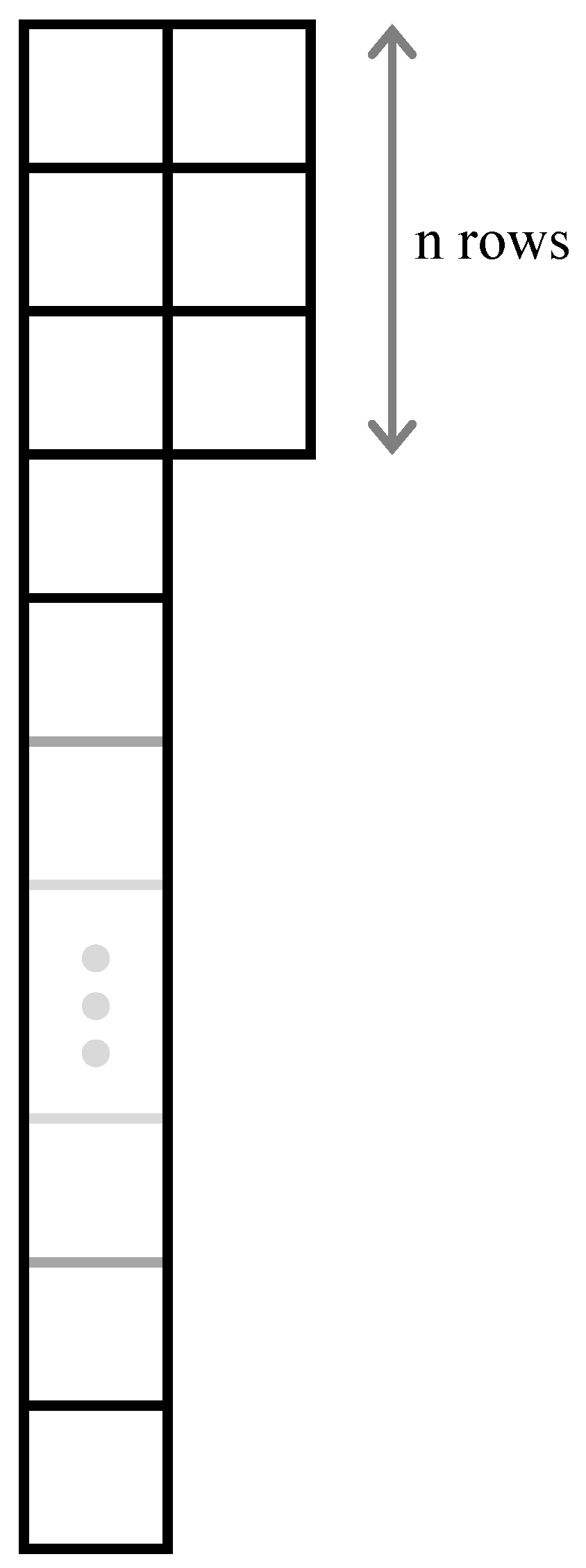
Although no local, relativistic Quantum Field Theory can describe a violation of PEP [15,16], we still need a theoretical frame for the interpretation of the experiment, and in particular of the nature of the electrons in the mixed symmetry state. To this end, we turn to the proposal of Rahal and Campa [17], who described a framework of PEP violation in non-relativistic quantum mechanics where the symmetry of global electronic wavefunction is described by a Young tableau as in Figure 1. This fits well with the Ramberg and Snow experiment, most of the electrons are antisymmetric with respect to the others, while a few (a fraction ${\beta }^2/2$) have symmetric wavefunctions with respect to particle exchange. In other words, there are anomalous electron pairs that have the wrong symmetry pairing, that cannot be changed by any physical process with a Hamiltonian, which is symmetric with respect to particle exchange (see also [18] for a more detailed discussion in the context of the VIP experiment).

3. Structure of the Semi-Analytical Monte Carlo Simulation of the X-ray Signal

We have already discussed how the signal of VIP and VIP2 develops in time for a fixed current in [14]. Here, we extend our treatment to time-varying currents with the aim of using current modulation as a tool to improve the accuracy of our measurements. From the calculations in [14], we know that the nonlinear nature of the problem leads to formulas that cannot be treated analytically to extract the final X-ray signal, and we must turn to a Monte Carlo simulation to find the average expected X-ray signal.

A simulation of the X-ray signal must take into account different sources of randomness: (1) The (small) number of anomalous conduction electrons (paired to corresponding atomic electrons inside the VIP2 target, from now on simply called anomalous electrons); (2) the arrival times of the anomalous conduction electrons; (3) the random motion of the anomalous conduction electrons in the whole conductor (both within and without the VIP2 target) that takes into account the time-dependent drift due to current modulation; (4) the spatial distribution of the anomalous atomic electrons. Next, we discuss each aspect in detail.

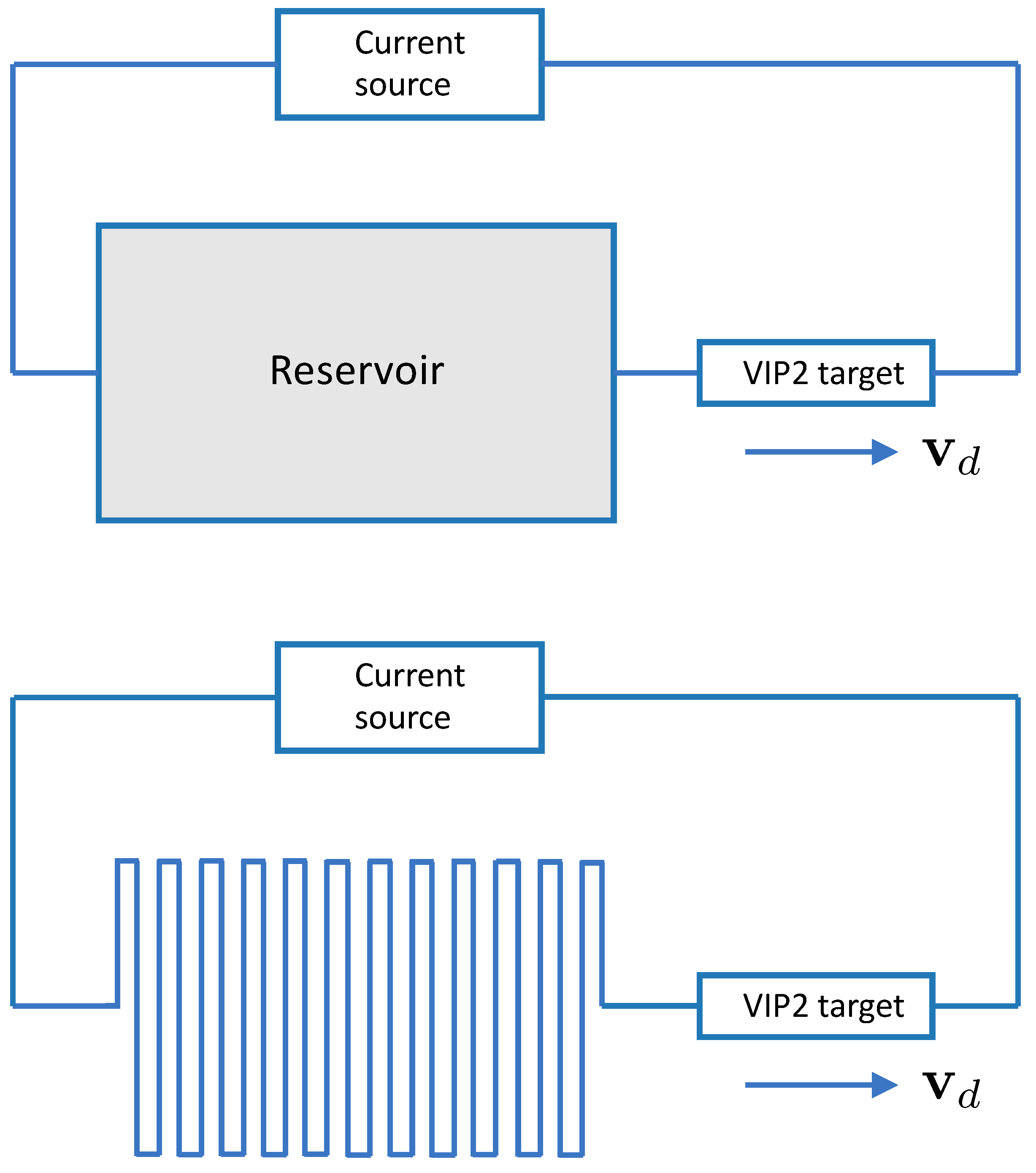
Since our aim is the estimate of the average signal, we adopt techniques that minimize the fluctuations of the Monte Carlo runs and boost computational efficiency. Since the total number of anomalous electrons only affects the amplitude of the signal, because of the linearity of the diffusion equation, we can fix this number in a given simulation run—i.e., we take a fixed fraction of all the electrons in the electric wire and in the block of metal that acts as “electron reservoir” (see Figure 2)—and thereby reduce the variability of the result. Moreover, this assumption allows to perform simulations with large numbers of electrons, and again it helps to reduce the relative fluctuation of the final result. We remark here that while in normal conditions, such as in the study of conventional solid-state problems, all the electrons in the material contribute to the physical effect being studied, and a simulation that takes into account each individual electron would be utterly unfeasible, in the present case we rely on the stringent existing bounds on the violation of the Pauli Exclusion Principle, so that we need to follow only a tiny fraction of all the electrons to simulate a realistic signal. Even with a bound as large as ${\beta }^2/2\lesssim {10}^{-28}$, close to that given in [8] for copper, we find that the number of violating electron pairs in one mole of copper is as small as $\sim {10}^{-4}$. Thus, taking a larger number of anomalous electrons, say of the order of ${10}^2$ or ${10}^3$ in the conducting wire loop, reservoir, and target, we obtain results that are suggestive of the expected signal fluctuations with reduced variability (which can still be scaled to lower numbers of anomalous electrons as we expect the amplitude of fluctuations to be proportional to the square root of the number of electrons).

The arrival times of the anomalous electrons correspond to different positions along the conductive leads that take them to the target. In this case, it is not natural to assume a priori that the spatial distribution is uniform and that the electrons are equally spaced because the subsequent random motion produces a spatial shift from the starting position that is a nonlinear function of time. Therefore, we take a uniform distribution of the anomalous electrons along the electric circuit and we let this initial configuration evolve in time while each anomalous electron performs a classical random walk in the circuit.

With a driving voltage, each conduction electron performs a biased random walk and—if simulated exactly—this random walk would also introduce an insurmountable difficulty because of the huge number of steps that are taken in the target [14]. However, as in [14], we can dispense with the full complexity of the process, and use the analytical formulas for the classical random walk instead. This is the most important variance-reduction choice in the simulation program—as the equations provide exact estimates of the average probability density of the anomalous electrons at any point and any time inside the VIP2 target. We also use the independence of motion along each direction, so that we neglect the transverse components of the random walk and take only the longitudinal component, with the corresponding one-dimensional estimate of the diffusion constant (one-third of the 3D constant, as only the longitudinal projection of motion matters in our formulation). Here we note that it is possible to take a 1D external circuit and ignore the transverse dimensions because electrons behave like an incompressible fluid, maintaining a constant current in the drift direction: an increase in the conductor section also means a corresponding decrease in drift velocity to maintain the current constant through each section of the conductor. We remark that this is the analytic step that makes the whole simulation semi-analytic.

The equations of the analytic part are based on the 1D diffusion-transport model for the classical random walk [19]. It is well-known that after injection a charge drifts and scatters (it undergoes transport and diffusion) so that the probability density of finding it at position $x=x\left(t\right)$ at time t—even the starting position $x\left(0\right)=x_0$—is

$$p\left(x\right|t)=\frac{1}{\sqrt{2\pi Dt}}exp\left[-\frac{{(x-x_0-x_S\left(t\right))}^2}{2Dt}\right],$$

(1)

which is the Green’s function of the diffusion equation for non-interacting classical random walks, see, for example, [20], where

$$x_S\left(t\right)={\int }_0^t{v}_d\left(t\right)dt,$$

(2)

is the total shift from the initial position of the random walker (the anomalous conduction electron), and where

$$v_d\left(t\right)=\frac{I\left(t\right)}{nezw}$$

(3)

is the time-dependent drift speed, which is related to the time-dependent current $I\left(t\right)$ and to the target properties (electron number density n; target thickness z; target width w). This means that the probability of actually finding one such electron in the target at time t is given by the integral

$$\begin{array}{cc}\hfill P\left(t\right)& ={\int }_0^L\frac{1}{\sqrt{2\pi Dt}}exp\left(-\frac{{(x-x_0-x_S\left(t\right))}^2}{2Dt}\right)dx\hfill \end{array}$$

(4)

$$\begin{array}{cc}\hfill & =\frac{1}{2}\left\{\mathrm{erf}\left[\frac{L-x_0-x_S\left(t\right)}{\sqrt{2Dt}}\right]-\mathrm{erf}\left[\frac{-x_0-x_S\left(t\right)}{\sqrt{2Dt}}\right]\right\}.\hfill \end{array}$$

(5)

Then, the probability that an anomalous electron is in the target at time t and is captured during a time span of duration $\Delta t$ is

$$P_X(t,\Delta t)={\int }_t^{t+\Delta t}P\left(t^{\prime }\right)\frac{e^{-(t^{\prime }-t)/{\tau }_C}}{{\tau }_C}d{t}^{\prime }\approx P\left(t\right)\left(1-e^{-\Delta t/{\tau }_C}\right)\approx P\left(t\right)\frac{\Delta t}{{\tau }_C}$$

(6)

where ${\tau }_C$ is the mean capture time (as defined in [18]), and where the approximation holds as long as $\Delta t\ll {\tau }_D$, where ${\tau }_D$ is the shortest drift time across the target computed from the maximum current amplitude in the modulation scheme. The capture probability $P_X(t,\Delta t)$ is also the probability of emitting an X-ray following the capture process.

The electrons perform their random walks along the circuit shown in Figure 2; the upper panel of Figure 2 shows the circuit that includes a large “electron reservoir”—a block of metal that is necessary to provide a sufficient supply of anomalous electrons—while the lower panel shows the circuit that is simulated by the program and where the drift speed is assumed to be uniform.

As shown in [14], close encounters between an anomalous conduction electron and the corresponding anomalous atomic electron almost inevitably lead to the formation of an anomalous pair in the target, with the emission of the corresponding tell-tale X-ray. However, it takes time before an anomalous electron meets its match, and this is taken into account by a proper absorption rate that translates into an absorption probability per time step, as discussed below.

The structure of the simulation program is straightforward, and the main steps of the C++ code are outlined in Algorithm 1. The generation of random numbers and the evaluation of special functions is handled by calls to the GNU Scientific Library [21].

Algorithm 1: Structure of the semi-analytical Monte Carlo for VIP2.

3.1. Modulation Schemes

Possible modulation schemes include the usual rectangular, triangular, sine, and sawtooth waves, and the numerical results of the Monte Carlo simulation can be used to select the best scheme to detect a possible violation of the Pauli principle.

To evaluate the signal-to-noise ratio of the harmonics in the frequency spectra we assume that the background noise is Gaussian. This assumption is reasonable, because electronics contribute to Gaussian noise, and this adds to the statistical Poisson noise, which can be regarded as Gaussian as well to a very good approximation level. In this scheme, we detect a violation when we find that there is a statistically significant spectral peak that corresponds to a harmonic of the current modulation frequency.

With the assumption of Gaussian noise we can use a well-known result in the theory of signals to evaluate the statistical significance of a violation [22], namely, that the probability density function (pdf) $p\left(S_k\right)$ of the periodogram $S_k={\left|F_k\right|}^2/N^2$, where $F_k$ is the discrete Fourier transform of the N samples $x_n$ taken at time $t_n=n\times \Delta t$:

$$F_k=\sum _{n=0}^{N-1}{x}_n{e}^{-2\pi nk/N},$$

is the exponential pdf

$$p\left(S_k\right)=\frac{e^{-S_k/({\sigma }^2/N)}}{{\sigma }^2/N},$$

(7)

(here ${\sigma }^2$ is the background noise variance). It is important to note that the mean value is $\langle S_k\rangle ={\sigma }^2/N$ and that the standard deviation of $S_k$ is ${\sigma }^2/N$, i.e., the standard deviation equals the mean value. Thus, a measurement of the mean value automatically yields also an estimate of the spectral standard deviation, which can be used to evaluate the statistical significance of a spectral peak.

4. Discussion

In this section we report preliminary, exploratory results from the simulation runs with the set of parameters listed in Appendix A. As explained above, the program includes a loop to average over the different initial configurations, which is iterated Nrepeats times, but in addition to this, there is another parameter—nrepeat—that acts as if the same initial configuration were run over and over again. The reason for introducing this additional option is that in exploratory runs there may not be enough X-ray events to allow an in-depth analysis of the spectral features of the X-ray signal. Taking a large value of nrepeat corresponds to assuming an unrealistically large data-acquisition time, but it provides a clear view of the signal shape and of the resulting frequency spectra.

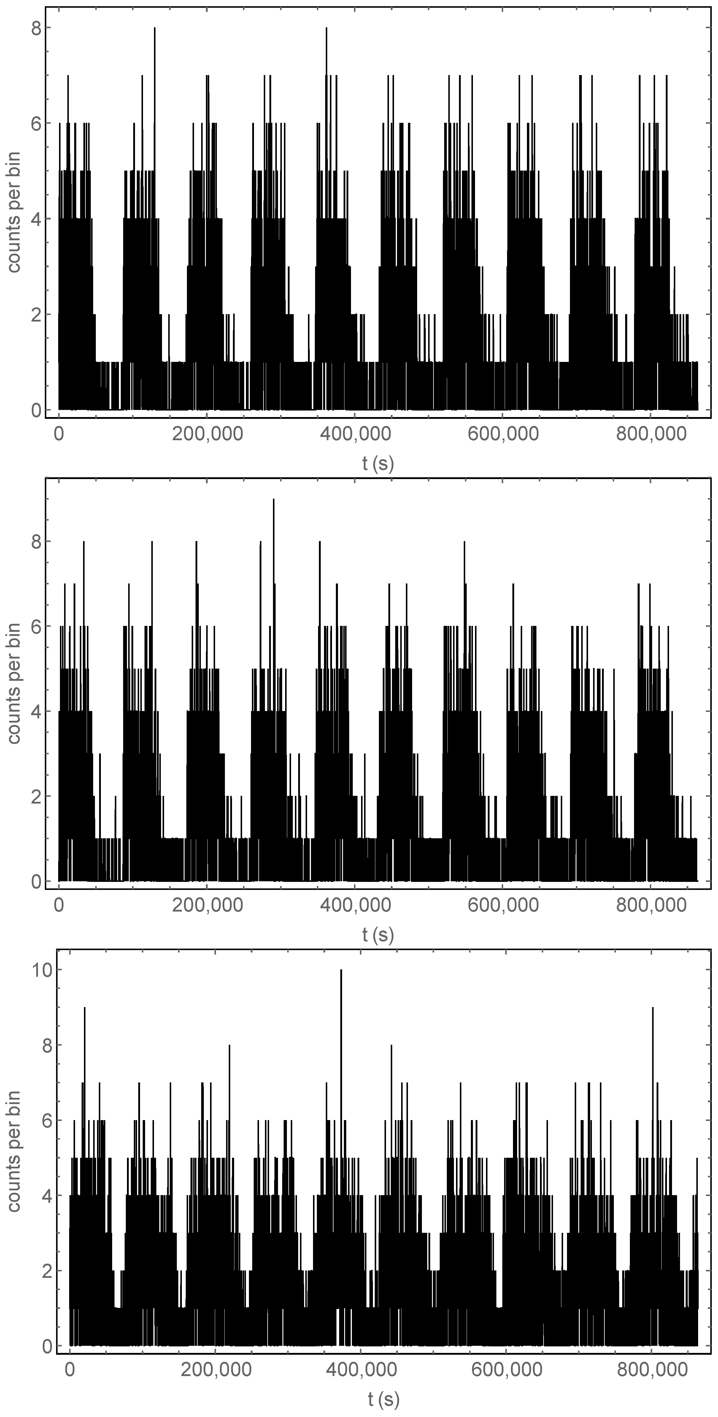
Figure 3 shows the time development of the sum of many (${10}^5$) X-ray signals over a data-taking time of 10 days, obtained with Nrepeats = 10 (10 different initial configurations) and nrepeat = ${10}^4$ (each configuration is used 10,000 times as the initial configuration), for different initial conditions and modulation types. In these simulations, we take T0 = 86,400 (a full current modulation period lasts 86,400 s, i.e., one day), so that each plot displays a total of 10 full current modulation periods (i.e., 10 days). The resulting total data-taking time of ${10}^6$ days is clearly impossible to achieve with a single target like the one simulated here; however, this points to a possible, very ambitious variant of the experiment, where the single target—with its associated detector—is replicated many times to produce summed signals such as those in Figure 3—with 10,000 replicas one could obtain the same total data-taking time in just 100 days.

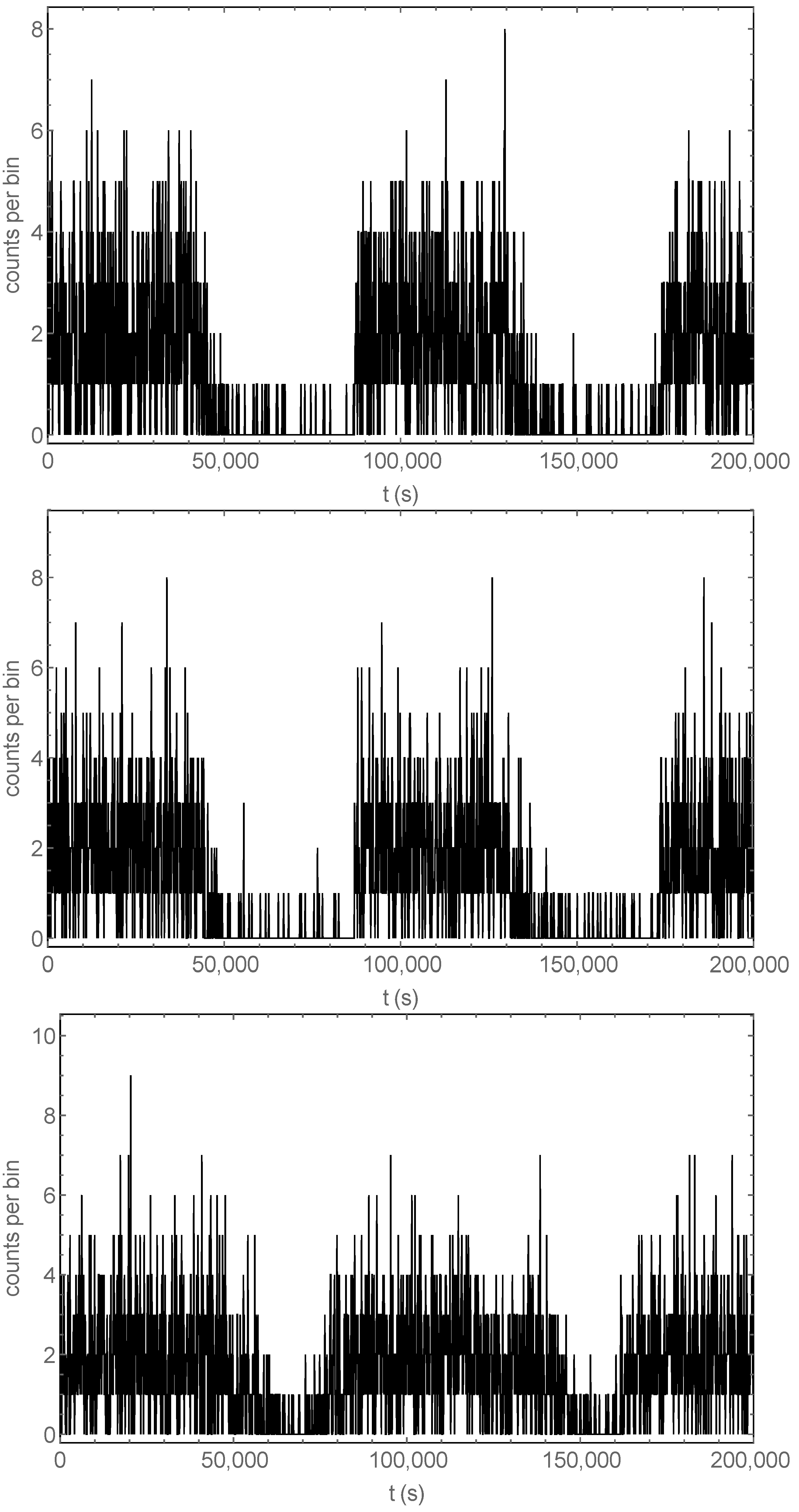
The sine wave current modulation is shown in the bottom panel of Figure 3, while the other two panels show a square wave modulation with different initial positions (randomly distributed and equidistributed anomalous electrons; the equidistributed case is not realistic but it has been included to display, by contrast, the effect of randomness in the initial distribution of the anomalous electrons). The square wave plots are less symmetrical than the one with the sine wave modulation and show a hint of a right tail after each peak. This is confirmed by the close-ups shown in Figure 4. This tail is the remnant signal from the anomalous electrons pushed into the target by the previous current-on cycle.

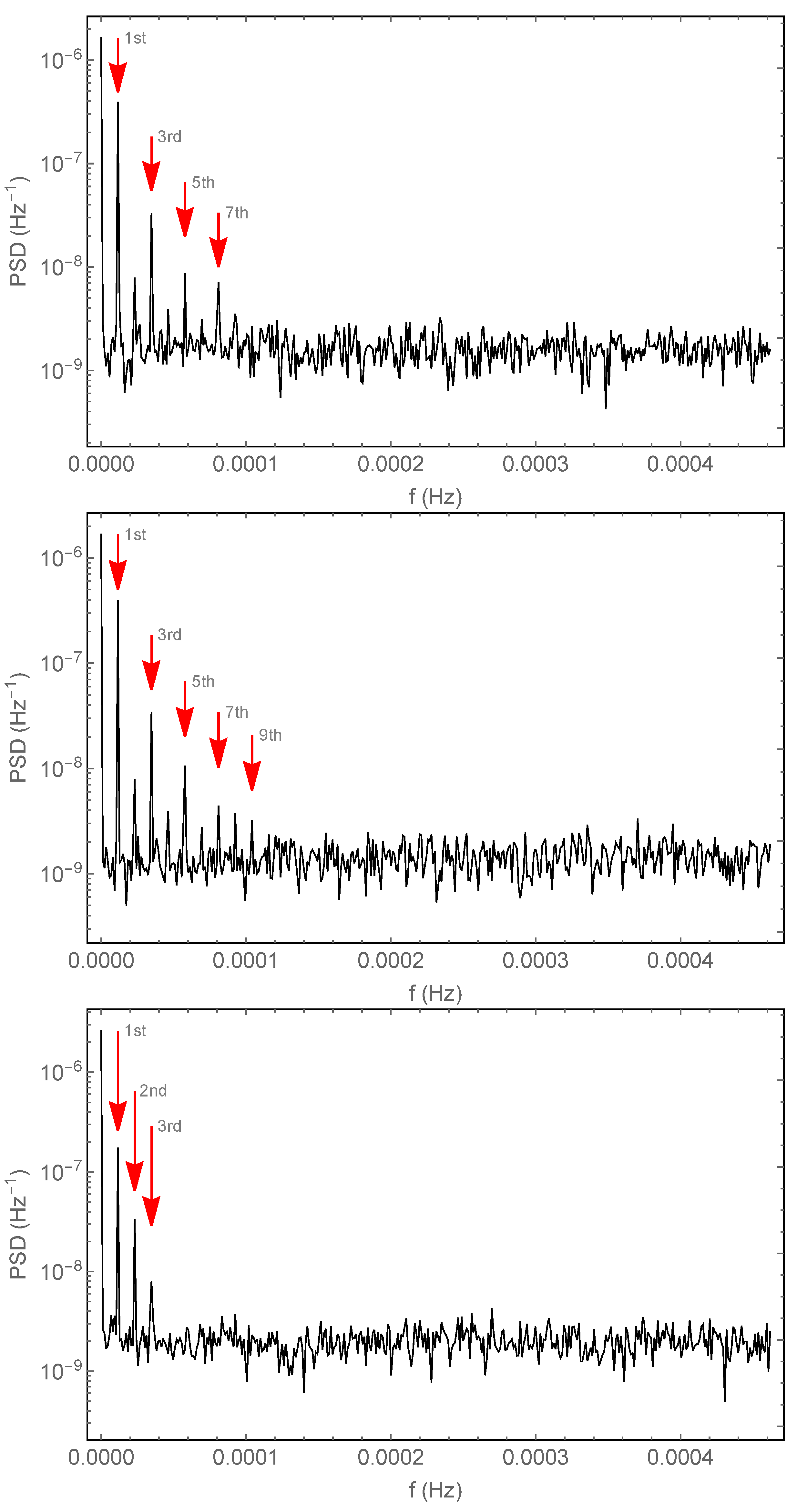
As discussed in the previous section, these signals are Fourier-analyzed and the resulting spectra are used to detect the physical signal and establish its statistical significance. Figure 5 shows the spectra obtained with the signals shown in Figure 3. We have already remarked that the time signals are somewhat distorted with respect to the driving current; therefore, it is not unexpected to find that the sine wave modulation, in addition to the expected first harmonic, displays peaks at the positions of the second and third harmonics (the other harmonics are drowned in the background noise). The square wave modulation is known to have only odd harmonics, and they are indeed well visible in both panels that refer to the square wave modulation. The center panel–which refers to the initially equidistributed anomalous electrons—has a slightly improved visibility for the odd harmonics. In the case of the square wave modulation, the distortion produced by the remnant signal in the current-off times shows up as small peaks at the even harmonics.

According to the discussion in Section 3.1, the mean background noise level also sets the significance of the peaks of the modulation harmonics. Consider for instance the top panel of Figure 5: in that case, the mean level is about $1.3\times {10}^{-9}{\mathrm{Hz}}^{-1}$, and this is also the standard deviation of the background noise. Then, from the figure we see that the 7th harmonic is about five standard deviations larger than the noise background and that all the odd harmonics, up to the 7th, plus the 2nd harmonic, could be used to detect a violation with better than $5\sigma$ significance (note that this may be optimistic—here we consider only the noise produced by the fluctuations of the very process that we wish to observe—we do not expect to find much electronic noise at the modulation frequency, and this is further decreased by averaging over many data-taking periods).

5. Conclusions

We have seen that the modulation method outlined in this paper solves some of the problems of the original analysis method of Ramberg and Snow. Here, we also remark that it allows overcoming yet another problem in the Ramberg and Snow experimental scheme, where one must define a Region of Interest (ROI) in the X-ray energy spectrum. This ROI critically depends on our estimate of the energy of the anomalous X-rays, and therefore on a deep theoretical understanding of the nature of a violation of PEP. In the present scheme, there is no need to be precise, since only the anomalous X-rays are modulated at the same frequency as the current, and therefore one can widen the ROI to be much more inclusive, and without critical hypotheses about the exact emission mechanism of the anomalous X-rays.

Finally, we note that—as stressed above—the results obtained in this paper must be viewed as a first exploratory glimpse into a landscape of possibilities. Several parameters must be tuned to find the most efficient way of modulating the current, and this shall be the goal of our future work, with the perspective of a large improvement in the accuracy of the bound on PEP violation.