
Developing an Optical Measuring System for Hole Saw Caps


1
Department of Industrial Education and Technology, National Changhua University of Education, Changhua 500, Taiwan
2
Department of Mechanical Engineering, National Chung Hsing University, Taichung 600, Taiwan
3
Department of Electronic Engineering, National Kaohsiung University of Science and Technology, Kaohsiung 807618, Taiwan
4
Program in Biomedical Engineering, Kaohsiung Medical University, Kaohsiung 80708, Taiwan
*
Author to whom correspondence should be addressed.
Symmetry 2021, 13(12), 2311; https://doi.org/10.3390/sym13122311
Submission received: 9 November 2021
/
Revised: 24 November 2021
/
Accepted: 29 November 2021
/
Published: 3 December 2021
(This article belongs to the Special Issue Selected Papers from IIKII 2021 Conferences)
Abstract
:This paper developed a set of size detection systems with a computer vision method based on the accuracy requirements of the hole saw caps to meet the needs of the accuracy detection machine. The results allow manufacturers to build a digitalized hole saw cap detection system at a low cost. We have designed a measurement system for the hole saw caps with the computer vision method to measure the dimensions of the hole saw caps. However, a valid measurement value of the hole saw caps must be positioned symmetrically. However, in fact, when the measurement system is positioned accurately asymmetrically, it will cause a problem in the measurement data. Therefore, the dark box environment made of a light source and the back plate of the hole saw caps material and two cameras are employed to observe the hole saw caps from both above and the side views. Then, personal desktop computers calculate the size of the hole saw caps based on the camera screen vision with a Python program. The results of the proposed methodology are obtained by measuring 10 workpieces of different sizes, and all the errors within a range of 2 pixels (pixel, px) met the detection standards. Therefore, the developed hole saw cap detection system is in line with expectations.
1. Introduction
In recent years, with the analysis of huge amounts of data and the popularization of Industry 4.0 and IoT (Internet of things) devices, various traditional factories have kept up with this wave, hoping to create greater benefits for enterprise, and to achieve data before analysis, one must have the ability to digitize the product. Hole saw caps (hole saw caps) are currently measured manually, so this paper attempts to develop an optical inspection system for the hole saw back caps, hoping to quickly saw the holes in a convenient way. The manufacturer currently uses optical instrument projection and some jigs to measure the size. This process requires a lot of manual processing and will take a lot of time. Therefore, the manufacturer hopes that the operation process can be as simple and fast as possible to saw the size data of the hole saw caps. The size and information of the cover are digitized to facilitate subsequent product analysis and product history and for other purposes. In addition, the development of a measurement system of the hole saw caps requires all measurement subjects to be constructed symmetrically and harmoniously in order to pursue the overall optimization of the hole saw cap measurement data.
In this research, we designed and produced a special optical measurement platform for the hole saw caps. This research uses Solidworks to design the optical platform mechanism [1], design the machine structure on Solidworks, and communicate with the manufacturer after the design is completed with regard to whether the steps, accuracy, and structure of the optical inspection platform meet the requirements of the manufacturer. The software tools consist of the programming languages C [2] and Python; Python packages NumPy [3], Matplotlib, SciPy, imutils, and Cloudan; database CouchDB [4]; computer vision libraries OpenCV and Atom IDE (integrated development environment); and git management software GitKraken [5]. The tools include the power supply RIGOL DP832, a desktop computer, a monitor, a light source for inspection, a paper box, a C920 camera, and a vernier caliper. These tools are used for writing hole saw cap measurement programs and combine the mechanisms of inspection to achieve the goal of the hole saw cap measurement system.
Automated optical inspection (AOI) is a technology based on machine vision as the inspection standard. The composition of the AOI inspection system is divided into six parts—camera, lens, light source, computer, mechanism, and electronic control—along with appropriate image processing algorithms to achieve the goal [6]. Before selecting hardware, we must first set up the AOI workflow to understand the working distance, field of view (FOV), camera frame rate (frames per second, FPS), focus length (FL), depth of field (DOF), aperture, sensor size, sensor pixel size, magnification, resolution, lens mount, and camera calibration. When a physical object is captured by a camera as a 2D plane image at a certain point in the 3D space, optical aberration is caused by refraction. At this time, camera correction is required to correct the aberration generated during the projection process. Common aberration types include spherical aberration, coma, astigmatism, field curvature, and distortion [7]. Distortion can be divided into two types according to the axial direction, radial distortion, and tangential distortion. There are only two ways to correct distortion. One is to replace the lens with a telecentric lens to remove the distortion through optical means, and the other is to use mathematical means to remove the distortion. In the future, we will use both. The Zhang calibration method was mainly used to correct radial distortion and does not include tangential distortion [8]. Before the calibration method in [8] was introduced, the existing calibration methods were roughly divided into two categories. The first is photogrammetric calibration, which uses a calibration object of known shape and size to calibrate the camera. This method requires expensive calibration equipment to be achieved. The second is the self-calibration method. This method requires moving the camera in a static scene, taking multiple pictures, and then calibrating using a non-linear method. Although this method is convenient, it has poor robustness and low accuracy. The calibration method in [8] solves the above problems. It is easy to use and has high accuracy. One only needs to print out the chessboard and paste it on a flat surface or directly take the real chessboard, and one can perform the calibration. The calibration process is quite easy. The chessboard swinging multiple angles in front of the camera is taken side by side, and then the coordinates of the chessboard on the photo are input into the algorithm to obtain the data required for correction. OpenCV has already written Zhang’s calibration algorithm [9]. In OpenCV, with the function name calibrate-Camera (this is the camel case naming method, which is often used for program function name naming), the user only needs to set up the camera and obtain the chessboard with it. The size of the picture, the coordinates of the chessboard in the photo, and the specifications of the chessboard can be used to obtain calibration data using the calibrate-Camera function. In the field of mathematical numerical analysis, interpolation is a process or method of inferring new data points within a range through known, discrete data points. In this paper, we try to use interpolation for lens correction and compare Newton polynomials, Lagrange polynomials, and cubic interpolation. Based on the above, we have developed and designed a measurement system for the hole saw caps, which uses the computer vision method to measure the dimensions of the hole saw caps. The dark box environment is made of a light source and the back plate of the hole saw cap material, and two cameras are used to observe the hole saw caps from above and from the side. A personal desktop computer obtains the camera screen and uses the Python program to calculate the size of the hole saw caps and to display the measurement results. Recently, Nieslony et al. [10] have focused on research problems related to the surface topography and metrological problems after the drilling process of explosively cladded Ti–steel plates. However, the author evaluated the results of the topography of the material after the drilling process based on mechanical and electromagnetic methods. In the literature [11], the authors have considered a comparative analysis of the Sensofar S Neox 3D optical profilometer, Alicona Infinite Focus SL optical measuring system, and a digital Keyence VHX-6000 microscope on assessing the surface topography of the Ti6Al4V titanium alloy after finish turning under dry machining conditions. However, the surface topography of the materials has been evaluated in many studies, which often used different devices with different measuring methods. Therefore, it is impossible to compare the measuring equipment and techniques used.
Finally, we used the developed measuring system for the hole saw caps to measure the hole saw caps to verify the usability and effectiveness of the developed measurement system. Firstly, RIGOL DP832 is a programmable three-channel linear DC power supply (30V/3A*2, 5V/3A*1). It can supply the light source power of the detection system, and the voltage and current can be adjusted on the control panel to adjust the light source. The light source uses Eddie Vision Technology’s ring-shaped light source RI-140-45 green light and the backlight light source FL250-150 green light. Both of these light sources can be controlled by voltage. The computer specifications used in this study are an i5-9400 CPU (central processing unit), 32 GB (gigabytes) of memory, and the win10 21H1 operating system. The screen is a BenQ GL2580. The camera uses Logitech’s C920 camera. The camera has the UVC (USB video class) protocol that OpenCV supports. We can directly use the computer to execute OpenCV to control the camera’s exposure, resolution, transmission format, and other parameters. Although the 1920 × 1080 resolution of this camera is not enough for the inspection of the hole saw caps, the price is relatively low, and it is suitable for the prototype development of the hole saw cap measurement system. The vernier caliper is a tool for measuring the length of the workpiece, which can measure the length unit at the millimeter level. The method of use is to use the outer fixed surface on the caliper to measure the inner diameter, the inner fixed surface to measure the outer diameter, and the depth rod to measure the depth. In this study, the measuring tool described above will be used as the measurement standard to determine that the measurement result of the hole saw cap optical measurement system is accurate. However, the errors are all within the range of 2 pixels (1 pixel is equal to 0.07 mm), which meets the detection standards. We have developed a system that saves manpower and does not use jigs for direct measurement. Furthermore, we provide relevant industries with a suitable price (under USD 3000) and easy-to-use hole saw cap inspection methods.
2. Materials and Methods
2.1. Hole Saw Caps
A hole saw is a tool that can be installed on a drill bit and cut a circular incision into sheet metal. Hole saw caps have one hole and four through holes (PIN holes). Hole saw caps are formed by welding a saw blade on the hole saw caps. It can be seen from an obliquely upward angle that the saw blade has inclined grooves to carry dust out [12]. The holes in the hole saw caps are used to fix the circular cavity saw on the hexagonal drill shaft. The hexagonal drill shaft can push the pin forward through the screw mechanism. When the circular hole saw is locked on the hexagonal drill shaft, the pin can be pushed in and fixed, and the combined hole saw cap can be fixed on the electric drill for cutting.
2.2. Interpolation
In the field of mathematical numerical analysis, interpolation is a process or method of inferring new data points within a range through known, discrete data points [13]. In this paper, we try to use interpolation for lens correction and compare Newton polynomials, Lagrange polynomials, and cubic interpolation.
2.2.1. Newton Interpolation
Consider a set of continuation points with k + 1 numbers:
No two in the set are the same. Then, the Newton interpolation polynomial is
Then, the expression of Newton’s basic polynomial is
where and .
2.2.2. Lagrange Interpolation
Consider a set of continuation points with k + 1 numbers:
If no two in the set are the same, then the Lagrange interpolation polynomial is
Then, the expression of Newton’s basic polynomial is
2.2.3. Cubic Spline Interpolation
For a set of n + 1 continuous point data sets, cubic spline interpolation can be used.
Assume that
There is another function f that can pass through the data set , where
Therefore, each cubic polynomial requires four conditions to be established. For the n cubic polynomials that make up S, 4n conditions are required to determine it. The interpolation characteristic gives n + 1 conditions, and the internal data points give conditions: a total of conditions. The other two conditions require different conditions to be used in different situations. There are three types of boundary lines for the cubic spline difference: natural spline, clamped spline, and not-a-knot.
If it is a natural boundary, specify that the two derivatives of the two endpoints are 0, that is,
If it is a fixed boundary, specify the first derivative of the endpoint as A and B, that is,
If it is a non-nodal boundary, make the value of the third derivative equal to the value of the third derivative of, and the value of the third derivative of is equal to the value of the third derivative of, that is,
2.3. Four-Point Perspective Transformation
Perspective transformation (perspective transformation) refers to the use of the three-point collinear condition of the perspective center, the image point, and the target point to rotate the bearing surface (perspective surface) around the trace (perspective axis) by a certain angle according to the perspective rotation law. The original projection light beam is destroyed, and the constant transformation of the projection geometry on the shadow-bearing surface is still maintained. In short, it is to project a plane onto a specified plane through a projection matrix [14]. The perspective transformation formula is as follows:
where u and v are the original picture, and the picture has no depth; thus, w = 1. Use the perspective transformation matrix of the plane to obtain the projected .
2.4. HSV Color Space
HSV refers to hue, saturation, and value, respectively. It is a cylindrical color space. Compared with the traditional RGB method, HSV is more in line with human visual representation. The color space is as follows in Figure 1. This research can use this color space to filter the color space blocks needed. As shown in Figure 2, the brown in the background is cut out. The binarization diagram of the back cover of the hole saw caps to be measured is divided to facilitate the measurement of the size, as shown in Figure 2.
3. Results
3.1. Detection Systems
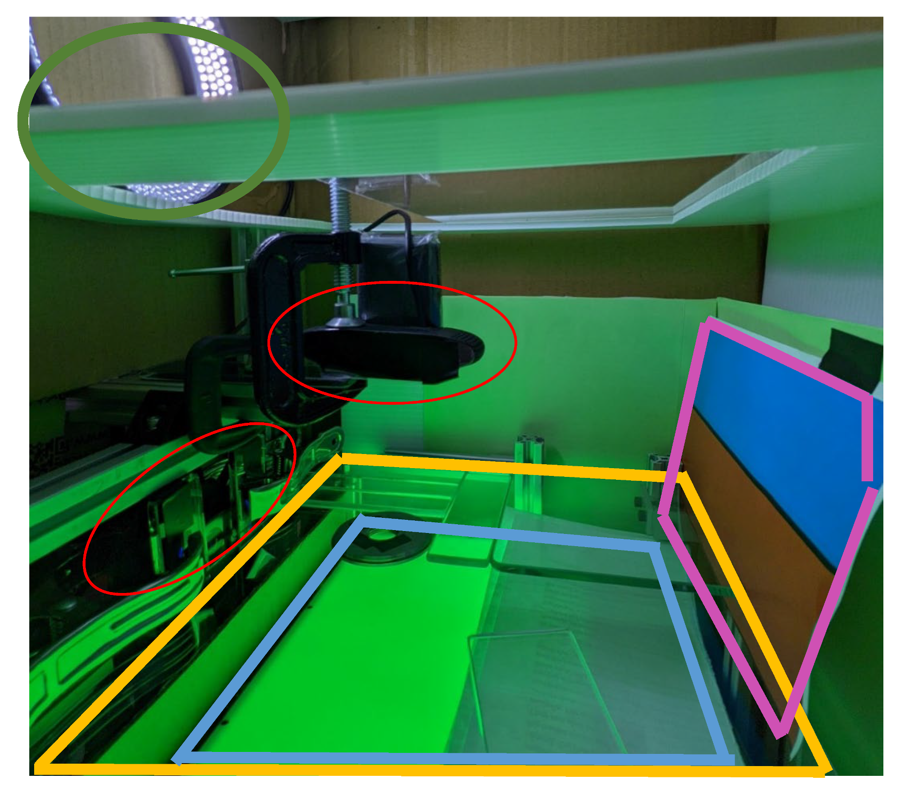
In order not to be affected by external ambient light, the detection system is designed with a dark box environment to keep the internal light source environment stable. The inside of the detection system is shown in Figure 3 with two Logitech C920 Pro cameras in the red area, and a white ring light source on the upper left. The orange area with a piece of background paper is in the pink area on the right, the purple area is the detection platform, and the light blue area is the green backplane light source.
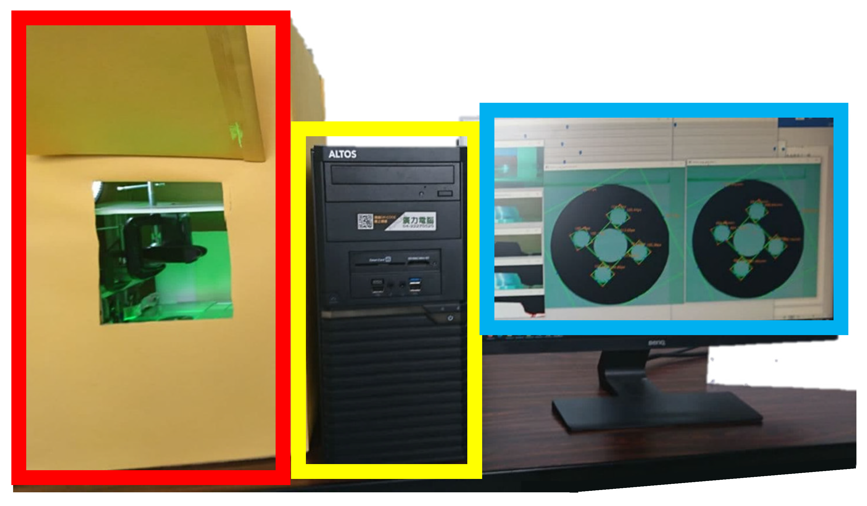
In Figure 4, the detection system camera in the red frame is connected to the desktop computer, the camera image can be sent to the computer for processing and analysis (the yellow frame in Figure 4), and the results are displayed on the screen (the blue frame). The light source power of the inspection mechanism is provided by the programmable power supply RIGOL DP832, as shown in Figure 5.
3.1.1. Camera
Two Logitech C920 Pro cameras are installed in the red circle as shown in Figure 3. One is placed on the top to look at the workpiece from the top, and the other looks at the workpiece from the side. The two lenses look at each other at 90°. The specifications of the C920 Pro camera are shown in Table 1. The diagonal field of view (dFOV) is 78°, and the resolution is 1920 × 1080. The horizontal and vertical viewing angles can be obtained by the following conversion formula, where dFOV (Df), Ha is the horizontal resolution (known value), and Va is the vertical resolution (known value).
Taking Ha = 1920, Va = 1080, and Df = 78° into consideration, the horizontal viewing angle Hf is 70.42796571601109°, and the vertical viewing angle Vf is 43.30672187287323°.
The hole of the detection platform in Figure 6 needs to be able to easily put in and take out the object to be tested with one hand, so it is necessary to reserve a certain amount of operating space. A height of about 10 cm can achieve this purpose through the experiment. Because the above needs to maintain a certain operating height, the working distance (WD) of the lens is set to 10 cm. Then, the object to be measured is placed on the detection platform, the size is measured optically to obtain the pixel (px) value of the size, and then the actual size is measured with a vernier caliper. After dividing the two values, the corresponding accuracy per pixel can be obtained. After calculation, the accuracy per pixel is 7.071688942891859. The detection accuracy of this study requires seven items in the minimum tolerance range. It needs to be at least three times the unit to meet the requirements of the accuracy: 7 divided by 3 equals . If we want to use higher accuracy in a formal working environment, the manufacturer must replace it with a higher-level camera.
3.1.2. Detection Platform
The inspection platform in Figure 7 is mainly composed of an aluminum extrusion and 29 cm long, 24 cm wide, and 5 mm thick glass. The platform is designed to use hexagon socket screws with heads on the aluminum extrusions at the four corners. This design allows us to use the rotating screw to adjust the height and use the spirit level to correct the level of the glass platform. The verticality and horizontality of the lens are first corrected by the aluminum extrusion to keep it level, then the glass is pressed against the aluminum to form a flat surface, and then the C-clamps and clamps are used to position the camera close to the glass surface.
In addition, we can also see that in addition to the workpiece to be tested on the glass platform, there are several rectangular glass pieces on the top, as shown in Figure 8. This is a specially designed combination set of glass pieces; these glass pieces are used to lean against the right side and bottom of the glass platform in Figure 7 and are measured, and then, when the workpiece is leaning on these glass sheets, the center of the workpiece can be kept in the middle of the visible range of the camera on the top of Figure 3 as much as possible. The principle that this set of special-sized glass pieces can keep the workpiece in the middle of the camera’s visible range is based on the file permission design of the Linux operating system. Linux file permissions are divided into three types: read, write, and execute. Their respective permission scores are 4 for reading, 2 for writing, and 1 for execution. If we want to give a file permission to read and execute, we add up their permission scores: 4 + 2 is 6. Similarly, if the file permission is given to be read and executed, then the file permission is 2 + 1, which is equal to 3. This is the minimum number, and the number of the key can represent the way of authority.
The detailed specifications of this set of glass sheets are shown in Table 2. Under the same principle, it is known that the largest outer diameter of the workpiece we want to inspect is 6 cm, and the smallest outer diameter is 4 cm. This set of glass sheets has been proven to be able to transfer the largest outer circle of 4~6 CM workpieces, all of which can be kept in the middle of the camera’s visible range.
Originally, acrylic material was used as the detection platform. Later, it was discovered that the workpiece to be tested would sag and cause inaccurate measurement after being put down. Therefore, 5 mm thick glass was used as the platform. After experiments, it was confirmed that the platform depression problem was solved.
3.1.3. Light Source
Some light sources in the laboratory are shown in Figure 9, which are a green backplane light source, a green ring light source, and a white ring light source. Machine vision light source notes [15] pointed out that if it is a silver metal object, green light and blue light are better choices, so we chose green light for our backplane light source.
The green backplane light source is placed at the light blue position in Figure 3. After experiments, as shown in Figure 10, it can be found that the contrast at the edge of the workpiece is very high, which is suitable for diameter size discrimination.
Inside the inspection system, at the red circle on the left side of Figure 3, there is a camera looking at the workpiece from the side. Since the hole saw cap is made of metal, it will be shown in Figure 11. The hole saw cap (left side of Figure 11) reflects green light. Therefore, the complementary colors of green and orange are used for the background plate to enhance the contrast and facilitate obtaining the size of the workpiece later.
3.2. Inspection Process
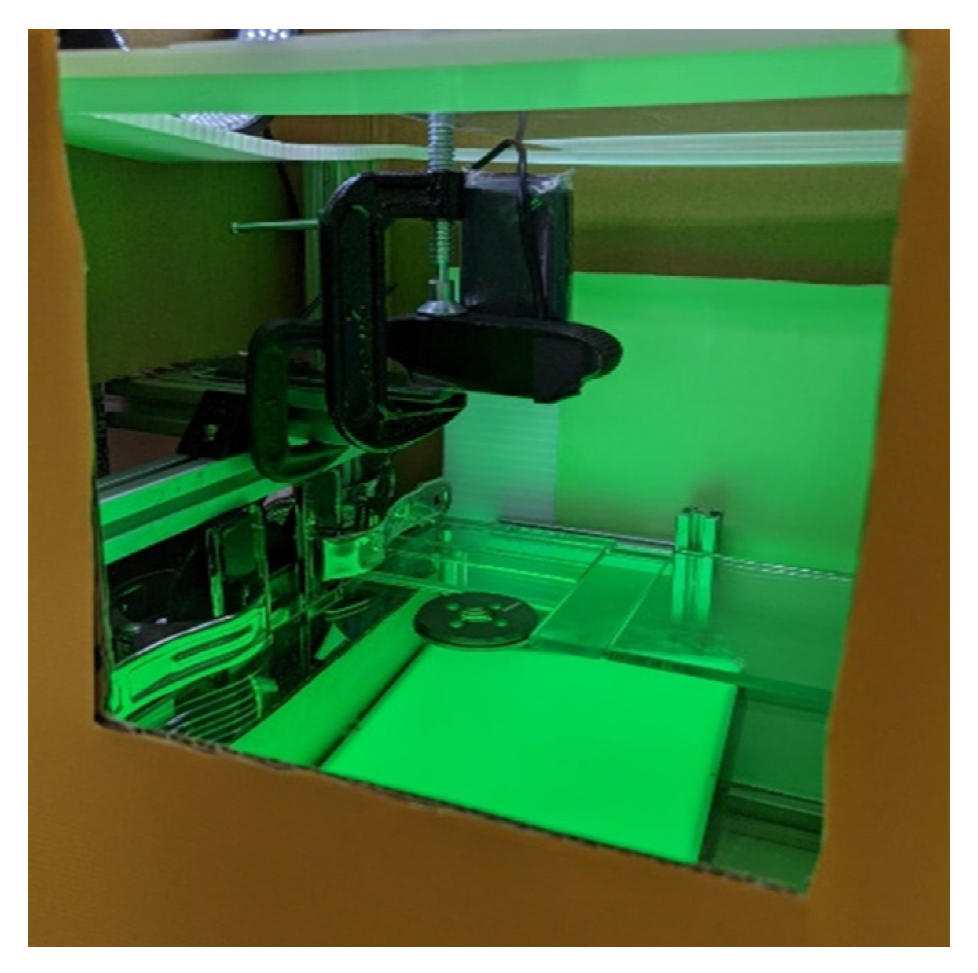
The manufacturer currently uses optical instrument projection and some jigs to measure the size. This process requires a lot of manual processing and will take a lot of time. Therefore, the manufacturer hopes that the operation process can be as simple and fast as possible to digitize the size of the hole saw caps. We have developed a system that saves manpower and does not use jigs for direct measurement. Figure 12 shows the detection mechanism from the outside to the inside.
Therefore, a convenient process is proposed here as shown in Figure 13. After the experiment, if the burr trimming and the time of CouchDB, the light source, and camera initialization are not considered, the detection process only takes 10 s.
3.3. Program Structure
As shown in Figure 14 above, the discrimination system requires the side camera and the top camera to start the program at the same time to operate.
3.4. Camera Calibration Method
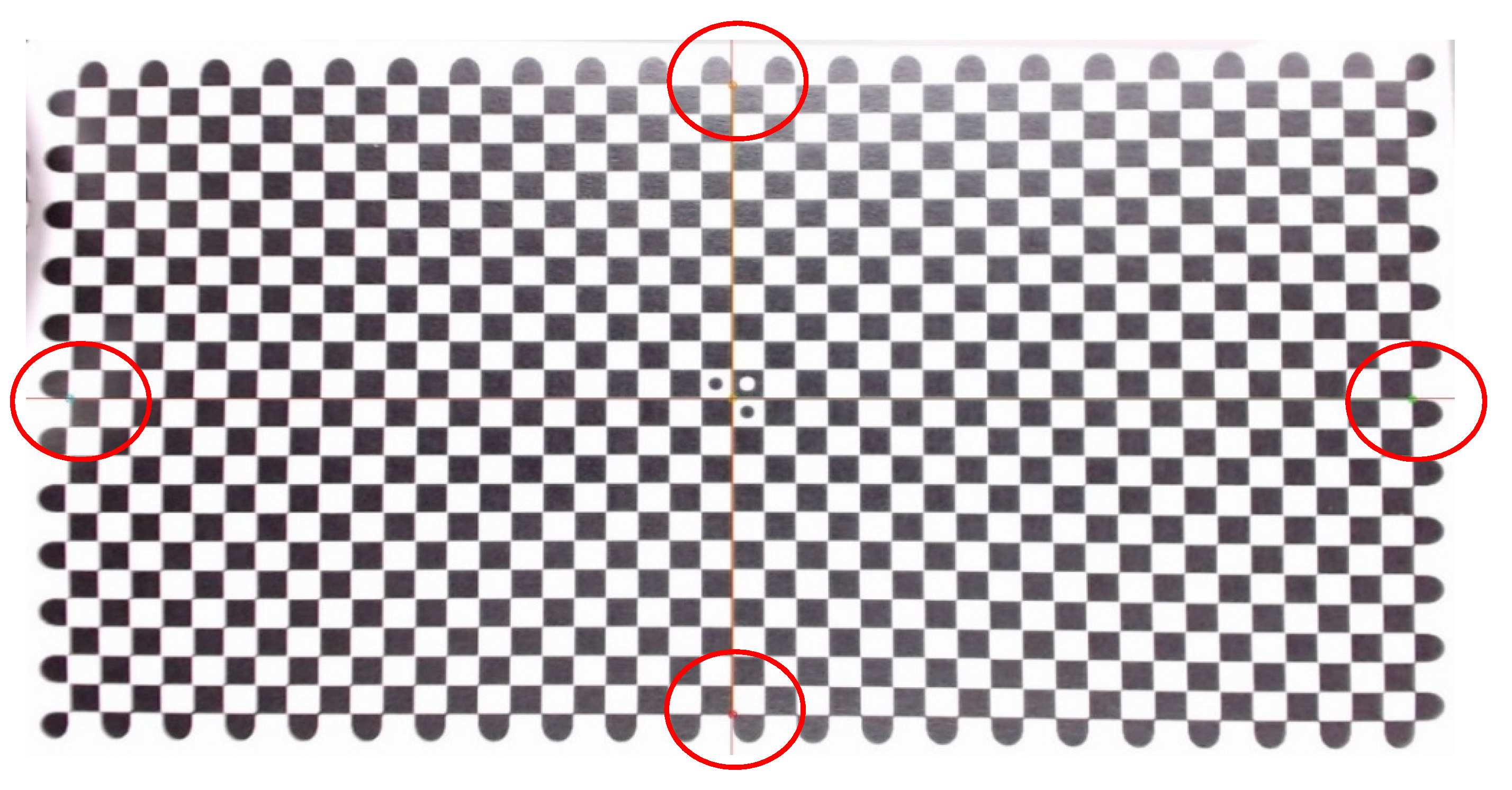
Following the introduction of camera calibration, this study uses OpenCV’s findChessboardCornersSB function to perform chessboard positioning, then uses calibrateCamera to generate the required data, and then uses getOptimalNewCameraMatrix to eliminate distortion. After the initial calibration, the red graph paper with equal intervals is placed on the detection platform, the red graph paper is pressed with the glass to make it flat against the detection platform, and then the calibration results are observed. The results are shown in Figure 15, with the blue box on the left. The internal standard vertical red line does not align with the lines of the red graph paper, indicating that the calibration has failed.
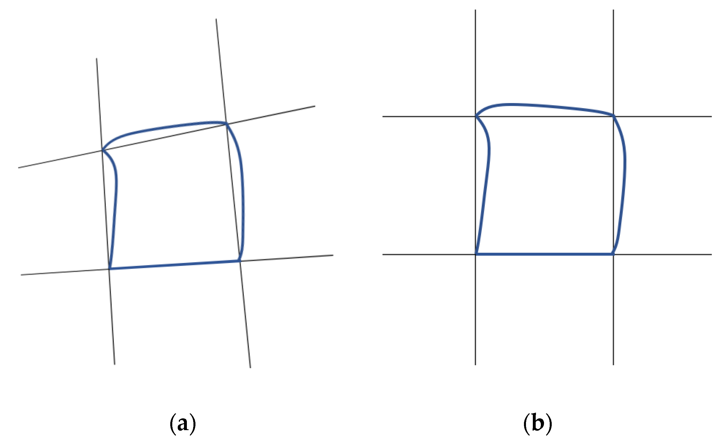
The application of the corrected getOptimalNewCameraMatrix function is canceled, and the original image aberrations are observed to obtain the distortion trend diagram in Figure 16. In Figure 16a, with regard to the deviation trend, it can be seen that in the first and fourth quadrants, it is normal. In the second quadrant, the upper line has a tendency of clockwise deflection. In the third quadrant, the lower the line, the more counterclockwise deflection tends to be. In Figure 16b, the deviation trend is only in the third quadrant, which is a normal straight line. The first and fourth quadrants deflect clockwise as they go to the right, and the second quadrant deflects counterclockwise as it goes to the left.
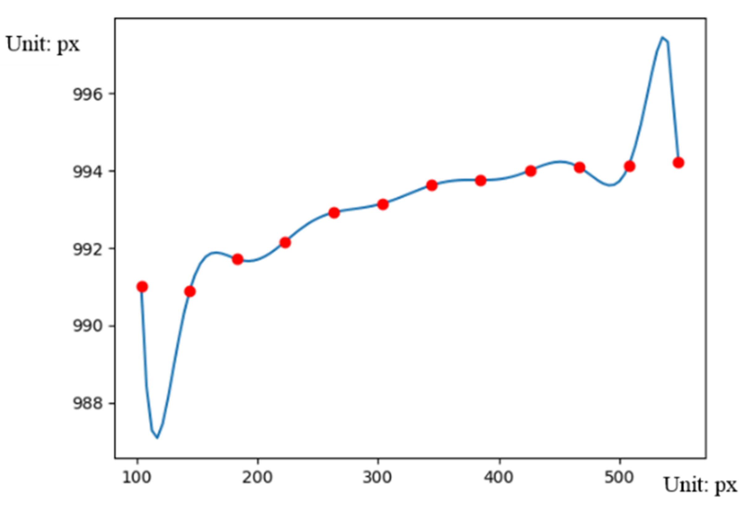
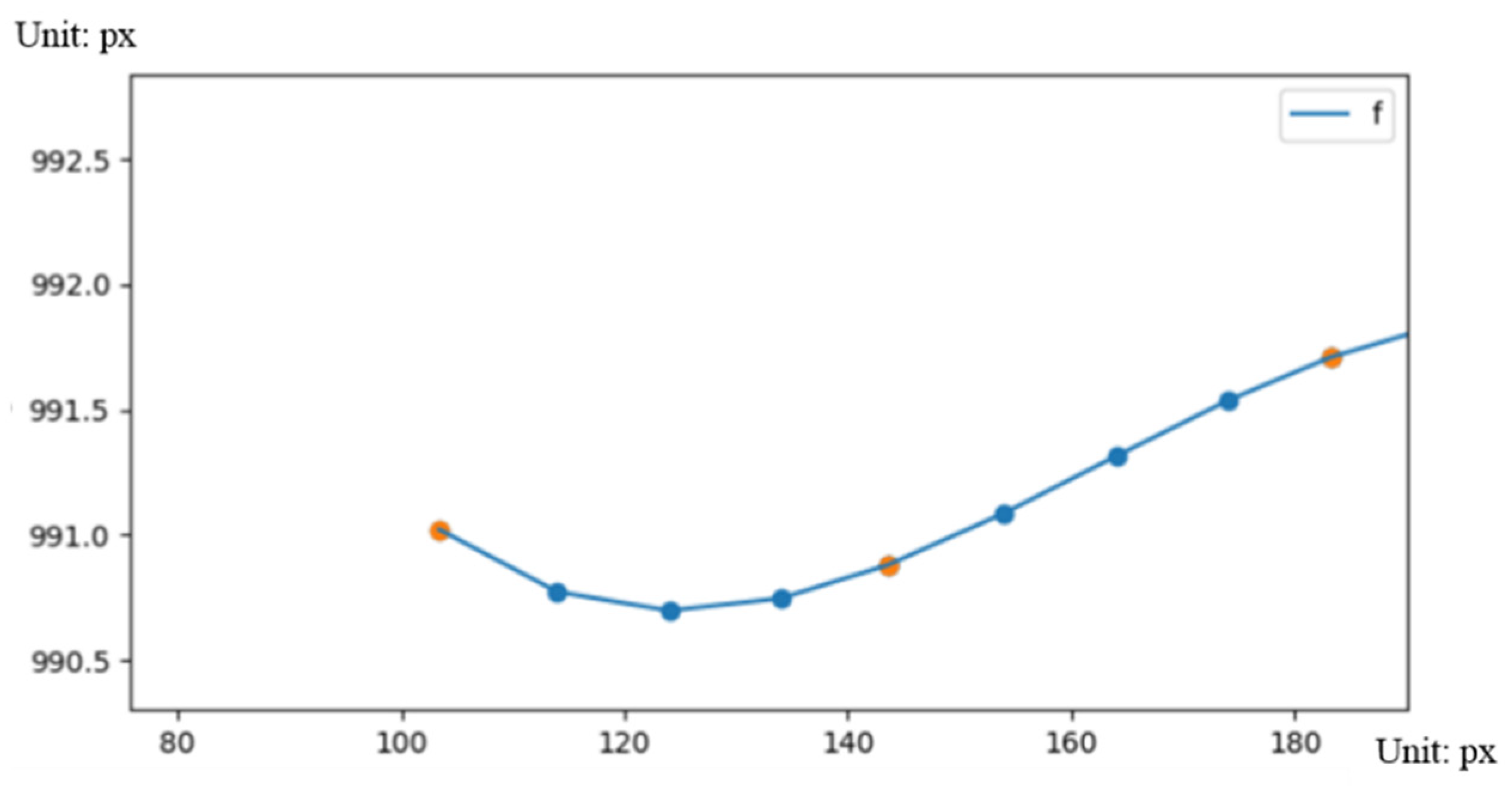
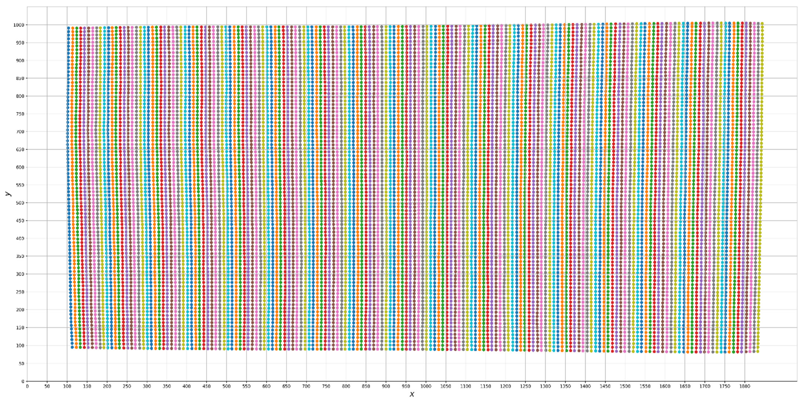
In order to obtain the exact value of distortion deflection, the red graph paper is changed to a 43 × 23 checkerboard chart dedicated to findChessboardCornersSB, the checkerboard chart is flattened with the glass, and then the self-made alignment program is opened, as shown in Figure 17. The program will grab the border. The intersection of the black and white squares is in the middle of the board (the red circle in Figure 17), and a circle mark is drawn on it. There are two standard red straight lines, one vertical and one horizontal, on the screen. The checkerboard is moved to make the intersection circle mark on the standard red line to complete the alignment. After the alignment is completed, the intersections of all black and white squares of the chessboard are determined, as shown in Figure 18, for digitization and analysis. After analysis, it is found that the outer boundary lines are not as regular as the quadratic curve, and there are repeated twists and turns, as shown in Figure 19. The actual coordinates of the boundary are captured numerically, and the red point is the junction point of the actual black and white squares of the chessboard.
It has been speculated that the market positioning of the C920 camera itself is a consumer-grade product, not an industrial camera, so the lens may not be required to be very flat, causing this situation. This research proposes a method to correct this situation. The method assumes that the checkerboard pattern has no protrusions on the inspection platform and is close to the glass inspection platform. As shown in Figure 20a,b, Figure 20a is the actual numerical coordinates of the checkerboard grid intersections. The intersections of the checkerboard grids are all distorted, and Figure 20b is a custom standard chessboard with the same average distribution size. A unit coordinate is assigned to the intersection of all checkerboards, the red dot in the middle is assigned the unit coordinate (0, 0), and the rest of the points are assigned in the Cartesian coordinate system according to the middle of (0, 0). Regarding the coordinates, for example, the orange dot on the upper left is assigned (−3, 3).
The four-point perspective transformation and the imutils package operation are used to make the picture’s (a) orange point coordinates (−3, 3), upper right blue point coordinates (−2, 3), lower right green point coordinates (−2, 2), and lower left yellow point coordinates (−3, 2), as well as the quadrilateral area enclosed by it. This is mapped and overlayed to the coordinates in Figure 20b. In this way, all the squares are mapped to the right coordinates to obtain the corrected image.
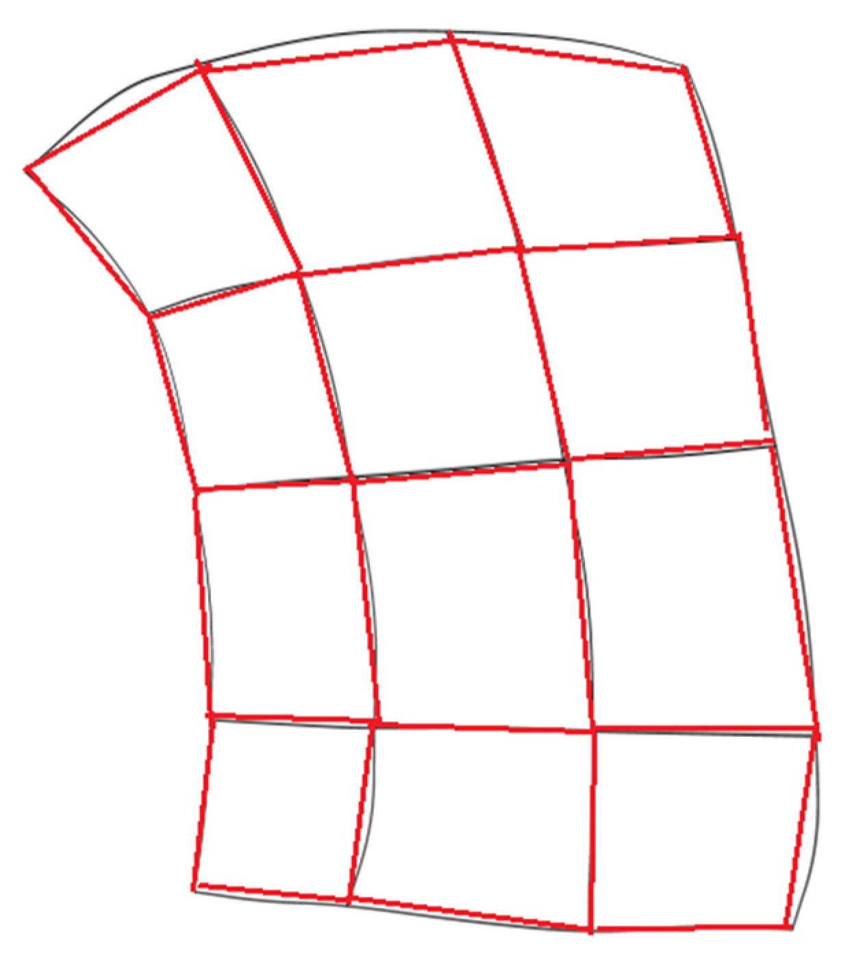
However, the corrected image obtained above has the situation of cutting and spilling as shown in Figure 21. Originally, in theory, the blue square in Figure 21a needs to be completely mapped. After the mapping, it will be found that the blue area in Figure 21b overflows to other blocks. If we want to improve, we can only increase the density of the segmented block, as shown in Figure 22, or use a higher-density checkerboard graph paper. However, because findChessboardCornersSB requires the grid to maintain a certain size for precise positioning, we can only choose the interpolation method. To increase the cutting density, we need to obtain the boundary line equation in the blue area of Figure 21b, but the boundary line equation cannot be obtained directly from the figure. Therefore, we need to obtain multiple point coordinates before interpolation.
After experiments, the Runge phenomenon may occur when using Newton’s method or the Lagrangian method [16], as shown in Figure 23; the boundary will oscillate, causing an inaccurate prediction of the boundary, which is a Runge phenomenon. However, using the cubic spline difference method for interpolation, the Runge phenomenon will not occur.
The equation of the boundary line has been interpolated from above. The length of the boundary curve can be obtained from this, and then the curve length can be divided into equal parts according to the desire to increase the splitting magnification. The principle is to first integrate the total length of each grid boundary, then divide the total length by the dividing block density magnification to obtain the specific value, and then re-segment integration to obtain the new position to be divided. Refer to the schematic diagram in Figure 24.
3.5. Size Measurement
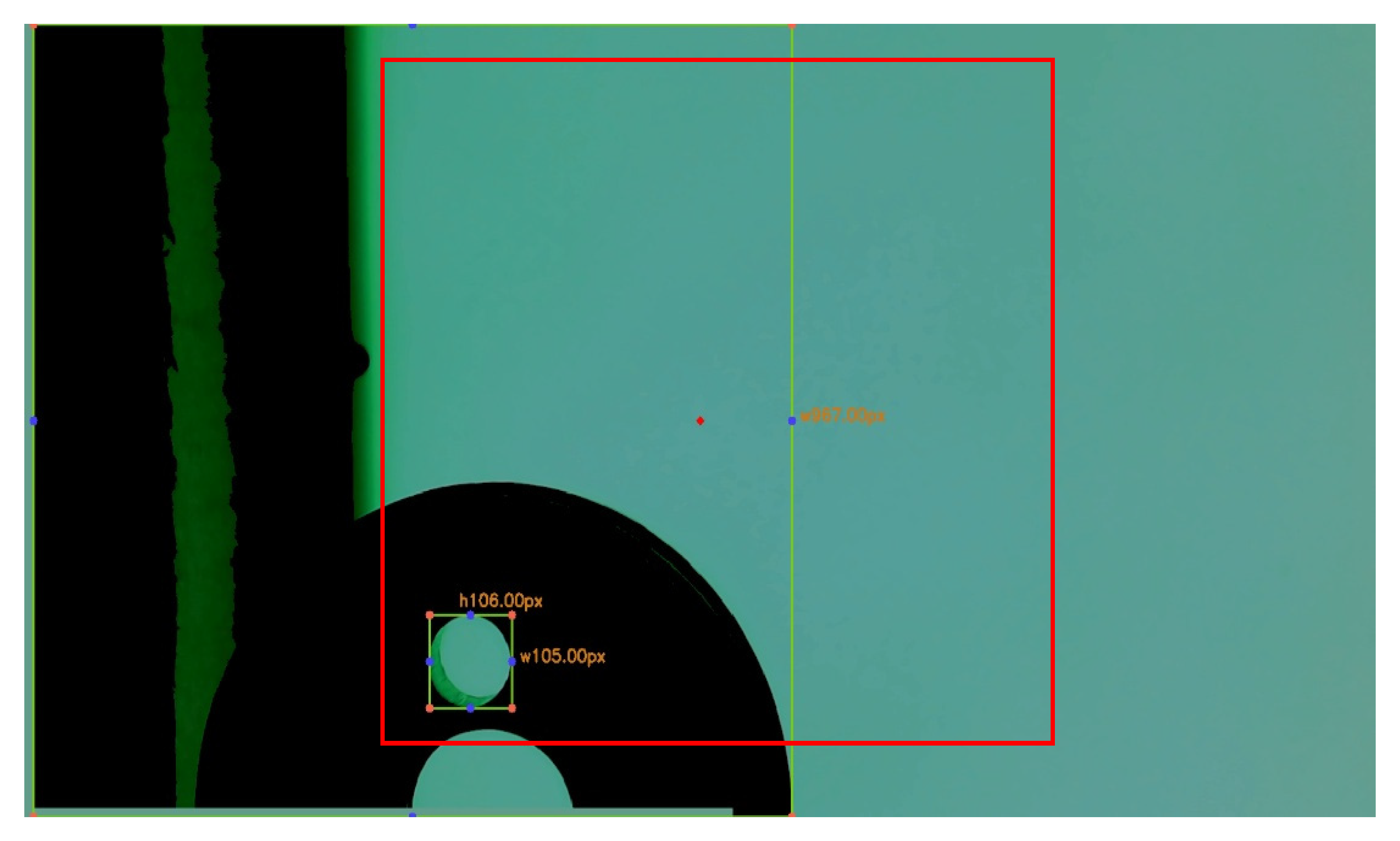
The size measurement needs to integrate the screens of the upper camera and the lower camera to determine. The red line in Figure 27 is a fixed boundary surrounded by an aluminum extrusion, the pink is the boundary of the object to be measured close to the glass, and the cyan is the diameter of the object to be measured perpendicular to the side camera and is the largest outer circle of the object to be measured. The dark blue is the distance from the side camera to the cyan line, and the yellow line is the distance from the cyan line to the pink line from the glass boundary.
Figure 28 is the screen of the upper camera measuring the size; the screen has the size detected in pixels. Figure 29 is the screen of the side lens measuring the size, the middle four images are used to detect the results of separation from the background, and in the area with the title bar img2 in the lower right corner, one can see the red dot that grabs the boundary point, the yellow dot that grabs the highest point of the object to be measured, and the green dot that grabs the maximum height of the outer circle of the object to be measured. The green and yellow dots are on the cyan line segment in Figure 27, that is, the maximum diameter of the lens on the parallel side of the test object. The upper layer of the thickness of the back cover of the circular hole saw is connected with the red dot, and the starting point of the slope change is indicated by the yellow dot. As shown in Figure 29, the lower layer of the thickness of the back cover of the circular hole saw is the hour when the slope changes after the red dots are connected, which are marked with green dots, as shown in Figure 29.
The size calculation process is as follows:
- Place the test object exactly on the border of the pink line in Figure 27.
- The upper lens uses HSV to segment the desired image and obtain the PIN hole, the outer diameter size.
- Divide the outer diameter by two to obtain the length of the yellow line in pixels in Figure 27.
- Obtain the pixel number counted from the bottom of the yellow point and the green point from the side camera.
- After recording, use a vernier caliper to measure the actual dimensions of the object to be measured.
- Because the actual coordinates of the green and yellow points and the corresponding height in pixels are known, a linear relationship can be established, and the actual size and thickness can be restored according to this ratio. This linear relationship is based on the same length as the yellow line in pixels in Figure 27. The next step will be valid under different lengths of the yellow line segment.
- Take another piece of the object to be tested with the same height and thickness but different outer diameters and perform steps 1–6. So far, two dimensions with the same height and thickness but different lengths of the yellow line segment have been obtained. These two can establish a linear relationship to calculate the actual size.
4. Discussion
4.1. Analysis of Lens Correction Results
After experimenting, using two times the interpolation magnification, Figure 30 shows the horizontal correction, and Figure 31 shows the vertical correction. The correction results of these two pictures are shown in Figure 30. For the convenience of viewing, the picture has been turned 90° to the vertical state. From the perspective of Figure 30, in the upper left of Figure 30a before correction, it can be observed that the checkerboard grid is offset from the standard vertical green thin line, while in Figure 30b after correction, the checkerboard square is close to the standard vertical green thin straight line. Then, according to Figure 31, we can also see that the square of the board is offset from the standard vertical green thin straight line on the left of Figure 31a before correction. After correction, the checkerboard square in Figure 31a is closely attached to the standard vertical green thin line. Next, as shown before, after comparing all the segments one by one, the corrected checkerboard squares are all pasted along the standard vertical green thin line.
The actual measurement is carried out, as shown in Figure 32, and the other three PIN holes of the workpiece are sealed to avoid forgetting which hole is used for the measurement. After the tooth hole is a non-measurement target, it is not closed. It is in the red frame area of the working range in Figure 32. The back cover of the circular hole saw is moved as much as possible, and the PIN hole size in the back cover of the circular hole saw is tested with regard to whether it is normal within the working range. The result shows that the calibration was successful. In addition, the calibration results using three and four times interpolation magnifications are not much different from two times, but if we use three or four times interpolation magnifications, the Python program may become stuck, and we need to rewrite the calibration program into the C language. In order to eliminate the lag situation, because we only use Python to write, we will not use three or four times to measure.
4.2. Analysis of Measurement Results
Table 3 is shown below. It is the measured value made by measuring the 10 hole saw caps in Figure 33. Each measurement object is labeled and affixed with white tape for calibration, as shown in Figure 34. After putting them into the measuring platform of the hole saw caps, the white marks are all facing forward, so that the four PIN holes are arranged up and down and left and right. The measurement environment has been calibrated for the horizontality and verticality of the camera, the levelness of the platform, and the arrangement of the platform glass group. After the power is turned off, it presents a completely dark box environment. It provides a 3 A/15.90 V green backplane light source and 3 A/18.07 V white ring light source power supply for detection under the light source environment.
In Table 3, Table 4, Table 5, Table 6 and Table 7, the same hole saw caps are used, and the measurement is repeated three times while maintaining the same position and angle. The three measurements show the same size and are reproducible, as shown in Figure 35.
The manual measurements in Table 3, Table 4, Table 5, Table 6 and Table 7 are measured with a vernier caliper, and the optical measurement is measured by the measurement system of the hole saw caps in this paper. The three columns of manual measurement are optical measurement. There is no unit in the gap/u column. The u represents the upper camera image measured by the hole saw caps. One pixel represents a few lines, and the u here is 7.0716889 lines.
In Table 3, Table 4, Table 5, Table 6 and Table 7, the gap in the outer diameter column of the hole saw caps gap/u only has a value of 3, exceeding 2, which means it exceeds the range of 1 px before and after the outer diameter of the hole saw caps. After checking the hole saw caps of label 3, it is found that there is no bottom burr, removed cleanly, causing the back cover not to fit the inspection platform. After trimming the burrs again, the measured gap/u is 1.131, which is lower than 2, so it is within the allowable range. This means that the test results of the measurement system for the hole saw caps developed by this research meet the requirements and are effective. We have developed a detection system for hole saw caps, which has met expectations. In the future, we will provide the relevant industries more affordable and easier-to-use hole saw cap inspection methods.
5. Conclusions
In this paper, the measurement of the hole saw caps is digitized, so a fast optical inspection platform for the hole saw caps is developed, and the software and interface for real-time detection of the hole saw caps are written using Python and OpenCV. This allows users to easily digitize the size of the back cover of the hole saw. The result shows that the same workpiece is measured at the same position and angled at the same position, and the displayed measurement size is the same, which is reproducible. This paper also proposes a dedicated “fixed plane angle platform camera image correction algorithm”, which is proved to be effective and usable through experiments, and the accuracy can be improved according to the measurement needs. On the whole, the development of a detection system for the hole saw caps meets expectations. The errors of the detection system are all within the range of two pixels (one pixel equals 0.07 mm), which meets the detection standards. In the future, we will provide relevant industries with a suitable price (under USD 3000) and easy-to-use hole saw cap inspection methods. Based on the results obtained, the following conclusions are drawn:
- (1)
- Aperture parameters of the hole saw caps are strongly dependent on the type of optical instrument projection and some jigs to measure the size.
- (2)
- The design of inspection platform allows us to use the rotating screw to adjust the height and use the spirit level to correct the level of the glass platform. The verticality and horizontality of the lens are first corrected by the aluminum extrusion to keep it level, then the glass is pressed against the aluminum to form a flat surface, and then the C-clamps and clamps are used to bring the camera close to the glass surface. Then, when the workpiece is leaning on these glass sheets, we try to keep the center of the workpiece in the middle of the visible range of the camera above. This set of glass sheets has been proven to be able to transfer the largest outer circle of the 4~6 CM workpieces, all of which can be kept in the middle of the camera’s visible range. At present, manufacturers use optical instrument projection and some jigs to measure the size. This process takes a lot of time because it requires a lot of manual processing.
- (3)
- For computer vision, if it is a silver metal object to be tested, green light and blue light are better choices, so we use green light as our backplane light source. It can be found that the contrast of the workpiece is very high, which is very suitable for diameter size discrimination. The inspection process only takes 10 s to complete a workpiece.
- (4)
- At present, the upper camera of the optical inspection platform is fixed at a designated position. In the future, a sliding rail can be added to allow the camera to move up and down freely to meet the needs of various types of hole saw cap size detection. In addition, it can have better rigid design for the mechanism. Currently, the calibration time is about 10 min before the experiment. It is hoped that the mechanism can be redesigned to greatly reduce the calibration time.
- (5)
- The main novelty of this work is a detailed comparison of modern optical computer vision and its measuring techniques using different measuring areas based on the measurements of aperture parameters on the example of hole saw cap finish measuring. It can be concluded that the most useful measuring equipment should be used according to specific technical requirements.
Author Contributions
(a) C.-Y.L., project administration, methodology, writing―original draft preparation. (b) T.-C.C., supervision. (c) L.-W.L., investigation. (d) R.-C.S., investigation. (e) T.-J.S., validation. All authors have read and agreed to the published version of the manuscript.
Funding
This research work was partly supported by the Ministry of Science and Technology, R.O.C., Grant No. MOST 110-2221-E-992-093.
Institutional Review Board Statement
Not applicable.
Informed Consent Statement
Informed consent was obtained from all subjects involved in the study.
Data Availability Statement
The data presented in this study are available on request from the corresponding author.
Conflicts of Interest
The authors declare no conflict of interest.
References
- Gracia, V.; Vergara, M. Applying action research in CAD teaching to improve the learning experience and academic level. Int. J. Educ. Technol. High. Educ. 2016, 13, 1–13. [Google Scholar]
- Ritchie, D.M. The development of the C language. ACM Sigplan Not. 1993, 28, 1–16. [Google Scholar] [CrossRef]
- Guttag, J.V. Introduction to Computation and Programming Using Python, 2nd ed.; MIT: Cambridge, MA, USA, 2016. [Google Scholar]
- Couchdb. 2021. Available online: https://docs.couchdb.org/en/stable/intro (accessed on 15 April 2021).
- Vasilescu, B.; Filkov, V.; Serebrenik, A. Stack Overflow and GitHub: Associations between software development and crowdsourced knowledge. In Proceedings of the International Conference on Social Computing, Alexandria, VA, USA, 8–14 September 2013; pp. 188–195. [Google Scholar]
- Wang, W.C.; Chen, S.L.; Chen, L.B.; Chang, W.J. A machine vision based automatic optical inspection system for measuring drilling quality of printed circuit boards. IEEE Access 2016, 5, 10817–10833. [Google Scholar] [CrossRef]
- Kirkpatrick, L.; Wheeler, G. Physics: A World View, 2nd ed.; Harcourt Brace College: Philadelphia, PA, USA, 1992. [Google Scholar]
- Zhang, Z.Y. A flexible new technique for camera calibration. IEEE Trans. Pattern Anal. Mach. Intell. 1999, 22, 1330–1334. [Google Scholar] [CrossRef] [Green Version]
- Camera Calibration and 3D Reconstruction. Available online: https://docs.opencv.org/2.4/modules/calib3d/doc/camera_calibration_and_3d_reconstruction.html (accessed on 17 March 2021).
- Nieslony, P.; Krolczyk, G.M.; Zak, K.; Maruda, R.W.; Legutko, S. Comparative assessment of the mechanical and electromagnetic surfaces of explosively clad Ti-steel plates after drilling process. Precis. Eng. 2017, 47, 104–110. [Google Scholar] [CrossRef]
- Leksycki, K.; Krolczyk, J.B. Comparative assessment of the surface topography for different optical profilometry techniques after dry turning of Ti6Al4V titanium alloy. Measurement 2021, 169, 108378. [Google Scholar] [CrossRef]
- Duda, A.; Frese, U. Accurate Detection and Localization of Checkerboard Corners for Calibration. In Proceedings of the 29th British Machine Vision Conference, Newcastle, UK, 3–6 September 2018. [Google Scholar]
- Camera Calibration. Available online: https://docs.opencv.org/master/dc/dbb/tutorial_py_calibration.html (accessed on 15 May 2021).
- Projection Matrix. Available online: https://en.wikipedia.org/wiki/Projection_matrix (accessed on 15 April 2021).
- Yashchuk, V.V. Performance Test of the Long Trace Profiler. Part 1: Random Noise Limit of Slope Measurement with Mirror M4 for BL 9.0.2. Light Source Note LSBL-710; ALS, LBNL: Berkeley, CA, USA, 2004. [Google Scholar]
- Boyd, J.P.; Ong, J.R. Exponentially-convergent strategies for defeating the Runge phenomenon for the approximation of non-periodic functions, part I: Single-interval schemes. Commun. Comput. Phys. 2009, 2, 460–472. [Google Scholar]
Figure 1.
HSV color space.

Figure 2.
HSV segmentation result.

Figure 3.
Inside the inspection system.

Figure 4.
Outside the inspection system.

Figure 5.
Monitoring agency light source power supply.

Figure 6.
Inspection platform opening.

Figure 7.
Glass platform.

Figure 8.
Special glass plate.

Figure 9.
Light sources.

Figure 10.
Result of using green light to illuminate the workpiece.

Figure 11.
Side camera result of using green light to illuminate the workpiece.

Figure 12.
External hole of inspection mechanism.

Figure 13.
Detection flow chart.

Figure 14.
(a) Side camera program; (b) upper camera program.

Figure 15.
The red graph paper after the first calibration.

Figure 16.
Schematic diagram of the distortion trend of (a) and (b).

Figure 17.
The actual screen of the checkerboard alignment program.

Figure 18.
Mark and digitize the intersection of all black and white squares of the board.

Figure 19.
Numericalization of the actual coordinates of the uppermost boundary.

Figure 20.
Schematic diagram (a) original graphics and (b) corrected graphics of correction method.

Figure 21.
(a) Original distortion; (b) after correction cutting overflow.

Figure 22.
Schematic diagram of increasing the cutting density.

Figure 23.
Interpolation using Newton’s method.

Figure 24.
Interpolation using cubic spline difference method.

Figure 25.
Interpolate the x-axis using cubic spline difference method.

Figure 26.
The y-axis is interpolated using cubic spline difference method.

Figure 27.
Dependency diagram of measurement platform.

Figure 28.
Upper camera to measure the size.

Figure 29.
Side camera to measure the size.

Figure 30.
(a) Horizontal measurement chart before correction; (b) horizontal measurement chart after correction.
Figure 30.
(a) Horizontal measurement chart before correction; (b) horizontal measurement chart after correction.

Figure 31.
(a) Vertical measurement chart before correction; (b) vertical measurement chart after correction.
Figure 31.
(a) Vertical measurement chart before correction; (b) vertical measurement chart after correction.

Figure 32.
Multi-point measurement after actual application of calibration.

Figure 33.
Hole saw caps.

Figure 34.
Hole saw caps after marking.

Figure 35.
Actual measurement result.


Table 1.
Camera C920 Pro specifications.
| dFOV (Diagonal field of view) | 78° |
| Maximum resolution | 1920 × 1080 |
| FPS (frame per second) | 60 |
| Lens type | Glass |
| Focus method | Variable focus |
| Transfer method | USB-A |
| Support agreement | UVC (USB video class) |
Table 2.
Glass sheet specifications.
| Specification (CM) | Quantity |
|---|---|
| 15 × 7 | 1 |
| 13 × 11 | 1 |
| 11 × 5 | 1 |
| 11 × 5 | 1 |
| 11 × 4 | 2 |
| 11 × 3 | 6 |
| 11 × 2 | 2 |
| 11 × 1.5 | 3 |
| 11 × 1.4 | 3 |
| 11 × 1.3 | 3 |
| 11 × 1.2 | 3 |
Table 3.
Hole saw caps outer diameter.
| u = 1 px Represents How Many cmm | U = 7.0716889185 | |||
|---|---|---|---|---|
| How Saw Outer Diameter | ||||
| No. | Manual Measurement | Optical Measurement | Disparity | Disparity/u |
| 1 | 5240 | 5229 | 11 | 1.55498 |
| 2 | 5238 | 5241 | 3 | 0.424227 |
| 3 | 5237 | 5222 | 15 | 2.121134 |
| 4 | 5240 | 5227 | 13 | 1.838316 |
| 5 | 5238 | 5239 | 1 | 0.141409 |
| 6 | 5239 | 5234 | 5 | 0.707045 |
| 7 | 5238 | 5232 | 6 | 0.848454 |
| 8 | 5238 | 5237 | 1 | 0.141409 |
| 9 | 5240 | 5231 | 9 | 1.27268 |
| 10 | 5238 | 5232 | 6 | 0.848454 |
Table 4.
PIN hole (upper).
| u = l px Represents How Many cmm | u = 7.0716889185 | |||
|---|---|---|---|---|
| PIN Hole (Upper) | ||||
| No. | Manual Measurement | Optical Measurement | Disparity | Disparity/u |
| 1 | 689 | 690 | 1 | 0.141409 |
| 2 | 690 | 690 | 0 | 0 |
| 3 | 690 | 692 | 2 | 0.282818 |
| 4 | 690 | 696 | 6 | 0.848454 |
| 5 | 690 | 697 | 7 | 0.989863 |
| 6 | 689 | 690 | 1 | 0.141409 |
| 7 | 688 | 694 | 6 | 0.848454 |
| 8 | 690 | 697 | 7 | 0.989863 |
| 9 | 688 | 690 | 2 | 0.282818 |
| 10 | 690 | 692 | 2 | 0.282818 |
Table 5.
PIN hole (right).
| u = l px Represents How Many cmm | u = 7.0716889185 | |||
|---|---|---|---|---|
| PIN Hole (Right) | ||||
| No. | Manual Measurement | Optical Measurement | Disparity | Disparity/u |
| 1 | 686 | 695 | 9 | 1.27268 |
| 2 | 687 | 693 | 6 | 0.848454 |
| 3 | 692 | 689 | 3 | 0.424227 |
| 4 | 688 | 695 | 7 | 0.989863 |
| 5 | 688 | 692 | 4 | 0.565636 |
| 6 | 688 | 690 | 2 | 0.282818 |
| 7 | 689 | 690 | 1 | 0.141409 |
| 8 | 688 | 695 | 7 | 0.989863 |
| 9 | 687 | 695 | 8 | 1.131271 |
| 10 | 688 | 696 | 8 | 1.131271 |
Table 6.
PIN hole (left).
| u = l px Represents How Many cmm | u = 7.0716889185 | |||
|---|---|---|---|---|
| PIN Hole (Left) | ||||
| No. | Manual Measurement | Optical Measurement | Disparity | Disparity/u |
| 1 | 686 | 684 | 2 | 0.282818 |
| 2 | 686 | 691 | 5 | 0.707045 |
| 3 | 690 | 693 | 3 | 0.424227 |
| 4 | 684 | 691 | 7 | 0.989863 |
| 5 | 686 | 695 | 9 | 1.27268 |
| 6 | 689 | 690 | 1 | 0.141409 |
| 7 | 686 | 691 | 5 | 0.707045 |
| 8 | 688 | 690 | 2 | 0.282818 |
| 9 | 687 | 690 | 3 | 0.424227 |
| 10 | 688 | 689 | 1 | 0.141409 |
Table 7.
PIN hole (down).
| u = l px Represents How Many cmm | u = 7.0716889185 | |||
|---|---|---|---|---|
| PIN Hole (Down) | ||||
| No | Manual Measurement | Optical Measurement | Disparity | Disparity/u |
| 1 | 685 | 681 | 4 | 0.565636 |
| 2 | 690 | 695 | 5 | 0.707045 |
| 3 | 690 | 685 | 5 | 0.707045 |
| 4 | 688 | 691 | 3 | 0.424227 |
| 5 | 690 | 686 | 4 | 0.565636 |
| 6 | 690 | 694 | 4 | 0.565636 |
| 7 | 688 | 685 | 3 | 0.424227 |
| 8 | 690 | 690 | 0 | 0 |
| 9 | 690 | 694 | 4 | 0.565636 |
| 10 | 690 | 688 | 2 | 0.282818 |
Publisher’s Note: MDPI stays neutral with regard to jurisdictional claims in published maps and institutional affiliations. |
© 2021 by the authors. Licensee MDPI, Basel, Switzerland. This article is an open access article distributed under the terms and conditions of the Creative Commons Attribution (CC BY) license (https://creativecommons.org/licenses/by/4.0/).
Share and Cite
MDPI and ACS Style
Lu, C.-Y.; Chang, T.-C.; Lee, L.-W.; Sung, R.-C.; Su, T.-J. Developing an Optical Measuring System for Hole Saw Caps. Symmetry 2021, 13, 2311. https://doi.org/10.3390/sym13122311
AMA Style
Lu C-Y, Chang T-C, Lee L-W, Sung R-C, Su T-J. Developing an Optical Measuring System for Hole Saw Caps. Symmetry. 2021; 13(12):2311. https://doi.org/10.3390/sym13122311
Chicago/Turabian StyleLu, Chien-Yu, Tsung-Chieh Chang, Lian-Wang Lee, Rong-Chu Sung, and Te-Jen Su. 2021. "Developing an Optical Measuring System for Hole Saw Caps" Symmetry 13, no. 12: 2311. https://doi.org/10.3390/sym13122311
Note that from the first issue of 2016, this journal uses article numbers instead of page numbers. See further details here.